Star formation in quasar hosts
and the origin of radio emission in radio-quiet quasars

Abstract

Radio emission from radio-quiet quasars may be due to star formation in the quasar host galaxy, to a jet launched by the supermassive black hole, or to relativistic particles accelerated in a wide-angle radiatively-driven outflow. In this paper we examine whether radio emission from radio-quiet quasars is a byproduct of star formation in their hosts. To this end we use infrared spectroscopy and photometry from Spitzer and Herschel to estimate or place upper limits on star formation rates in hosts of $\sim 300$ obscured and unobscured quasars at $z<1$. We find that low-ionization forbidden emission lines such as [NeII] and [NeIII] are likely dominated by quasar ionization and do not provide reliable star formation diagnostics in quasar hosts, while PAH emission features may be suppressed due to the destruction of PAH molecules by the quasar radiation field. While the bolometric luminosities of our sources are dominated by the quasars, the 160µm fluxes are likely dominated by star formation, but they too should be used with caution. We estimate median star formation rates to be $6-29$ $M_{\odot}$ yr^-1, with obscured quasars at the high end of this range. This star formation rate is insufficient to explain the observed radio emission from quasars by an order of magnitude, with $\log(L_{\rm radio,obs}/L_{\rm radio,SF})=0.6-1.3$ depending on quasar type and star formation estimator. Although radio-quiet quasars in our sample lie close to the 8-1000µm infrared / radio correlation characteristic of the star-forming galaxies, both their infrared emission and their radio emission are dominated by the quasar activity, not by the host galaxy.

1. Introduction

The most extended, powerful and beautiful sources in the radio sky are due to synchrotron emission from relativistic jets launched by supermassive black holes in centers of galaxies (Urry & Padovani, 1995), but only a minority of active black holes produce these structures. At a given optical luminosity of the active nucleus, radio power spans many orders of magnitude, and the exact distribution of radio luminosities remains a matter of continued debate. A particularly intriguing point is whether this distribution is bimodal (Ivezić et al., 2002; White et al., 2007; Kimball et al., 2011): does the brighter “radio-loud” population show a well-defined luminosity separation from the fainter “radio-quiet” group, or is the distribution of radio luminosities continuous (e.g., Bonchi et al. 2013)? This question goes to the heart of fundamental issues in black hole physics: are weak radio sources associated with supermassive black holes due to relativistic jets which are scaled down from their extended powerful analogs, or are there additional mechanisms for producing radio emission? Are all black holes actually capable of launching a relativistic jet, and do all black holes undergo such a phase?

At $\gtrsim 1^{\prime\prime}$ resolution, the majority of quasars ($L_{\rm bol}\gtrsim 10^{45}$ erg s^-1) are point-like radio sources with luminosities $\nu L_{\nu}[1.4{\rm GHz}]\lesssim 10^{41}$ erg s^-1, and the origin of this emission has been the subject of recent debate (Laor & Behar, 2008; Condon et al., 2013; Husemann et al., 2013; Mullaney et al., 2013). The recent finding of a strong proportionality between the radio luminosity of radio-quiet quasars and the square of the line-of-sight velocity dispersion of the narrow-line gas (Spoon & Holt, 2009; Mullaney et al., 2013; Zakamska & Greene, 2014) is an exciting development in this topic, offering possible clues as to the nature of the radio emission. These velocity dispersions can reach values that are much higher than those that can be confined by a typical galaxy potential, suggesting that the ionized gas is neither in static equilibrium nor in galaxy rotation. Blue-shifted asymmetries suggest that the gas is outflowing (Zakamska & Greene, 2014), and interpreting the line-of-sight velocity distribution as due to the range of velocities in the outflow suggests $v_{\rm out}\sim 1000$ km s^-1.

The observed correlation between narrow line kinematics and radio luminosity suggests a physical connection between the processes that produce them. One possibility is that compact jets inject energy into the gas and launch the outflows (Veilleux, 1991; Spoon & Holt, 2009; Mullaney et al., 2013); another is that the winds are driven radiatively, then induce shocks in the host galaxy and the shocks in turn accelerate relativistic particles (Stocke et al., 1992; Wang, 2008; Jiang et al., 2010; Ishibashi & Courvoisier, 2011; Faucher-Giguère & Quataert, 2012; Zubovas & King, 2012; Zakamska & Greene, 2014).

A completely different approach is followed by Kimball et al. (2011) and Condon et al. (2013) who argue that the radio emission in radio-quiet quasars is mostly or entirely due to star formation in their host galaxies. Three arguments could be put forward to support this hypothesis: (i) If the radio luminosity function is bimodal, then something other than scaled-down jets is probably responsible for the radio-quiet sources. (ii) Active galaxies with $L_{\rm bol}\lesssim 10^{45}$ erg s^-1 tend to lie on the extension of the classical 8-1000µm / radio correlation of the star-forming galaxies (Morić et al., 2010; Rosario et al., 2013). (iii) The amount of radio emission seen in high-redshift radio-quiet quasars can be explained by star formation rates $20-500M_{\odot}$ yr^-1, which (although quite high) seem plausible for the epoch of peak galaxy formation.

Several arguments can be put forward against this hypothesis: (i) In quasars, the scatter around the radio / infrared relationship is higher than that seen in star-forming galaxies (Morić et al., 2010). (ii) In quasars the infrared emission can be dominated by the quasar, rather than by the star formation (Hony et al., 2011; Sun et al., 2014). (iii) The amount of star formation required to explain the observed radio emission in quasars may be higher than that deduced using other methods (Lal & Ho, 2010; Zakamska & Greene, 2014).

Rosario et al. (2013) demonstrate that in radio-quiet low-luminosity active galactic nuclei (AGN) much of the observed radio luminosity is consistent with star formation in the AGN hosts. The objects in their sample have infrared luminosities $\nu L_{\nu}$[12µm]$\lesssim 10^{44}$ erg s^-1. In this paper we examine AGNs with $\nu L_{\nu}$[12µm] from $\sim 2\times 10^{43}$ to $\sim 10^{46}$ erg s^-1, thereby extending the analysis of Rosario et al. (2013) to luminosities higher by up to two orders of magnitude. Our goal is to determine whether the radio emission of quasars ($\nu L_{\nu}$[12µm]$\gtrsim 10^{44}$ erg s^-1, or $L_{\rm bol}\gtrsim 10^{45}$ erg s^-1 as per bolometric corrections by Richards et al. 2006) is due to the star formation in their host galaxies.

To this end, we estimate the rates of star formation in the hosts of quasars of different types using Spitzer and Herschel data, and compare the amount of radio emission seen from these objects with that expected from star formation alone (Helou et al., 1985; Bell, 2003). In Section 2 we describe sample selection, datasets and measurements. In Section 3, we use far-infrared photometry to calculate star formation rates, predict the associated radio emission and compare with observations. In Section 4 we use mid-infrared spectroscopy for a similar analysis. We discuss various difficulties in measuring star formation rates of quasar hosts in Section 5 and summarize in Section 6. We use a $h$=0.7, $\Omega_{m}$=0.3, $\Omega_{\Lambda}$=0.7 cosmology.

Throughout the paper, we make a key distinction between far-infrared ($\gtrsim 100\micron$) vs radio correlation and total infrared (conventionally defined over 8-1000µm range) vs radio correlation. For star forming galaxies which show similar infrared spectral energy distributions, these concepts can be used interchangeably, since an accurate estimate of the total infrared luminosity can be obtained from far-infrared fluxes alone (e.g., Symeonidis et al. 2008). However, as we add quasar contribution to both infrared and radio emission, some or all of these relationships might break down, and in particular because of the wide range of quasar spectral energy distributions their far-infrared emission and their total infrared emission are no longer strongly correlated. In Section 6, we investigate the fate of far-infrared vs radio and total infrared vs radio correlations in the presence of a quasar.

2. Samples, observations, data reduction and measurements

2.1. Type 2 and type 1 samples

Our goal is to assemble a large sample of quasars (whether optically obscured or unobscured) for which the host star formation rates can be usefully constrained with existing archival data. Furthermore, because of the sensitivity of the existing radio surveys, in order to probe the radio-quiet population we are restricted to low-redshift quasars, $z<1$. As a result, this work primarily focuses on the analysis of two quasar samples.

Our first sample consists of Spitzer and Herschel follow-up of obscured (type 2) quasars from Reyes et al. (2008) at $z\lesssim 0.8$. These objects are selected to have only narrow emission lines with line ratios characteristic of ionization by a hidden AGN (Zakamska et al., 2003) and are required to have $L_{\rm[OIII]}\gtrsim 10^{41.5}$ erg s^-1. Of the 887 objects in Reyes et al. (2008) catalog, WISE-3 matches are available for 94% of the objects and WISE-4 matches for 87% (some of the remaining 13% are detected, but cannot be deblended from the nearby contaminants in the WISE-4 band). We calculate 12µm luminosities from the WISE-3 matches, k-correcting using WISE-4 flux if available or using a median WISE-4/WISE-3 index if not (Zakamska & Greene, 2014).

For this sample, we collect archival Spitzer photometry and analyze new Herschel photometry as discussed in Sections 2.2 and 2.3 for a total of 136 objects. Furthermore, while we previously published ten Spitzer spectra of type 2 quasars (Zakamska et al., 2008), in Section 2.4 we conduct an extensive archival search which allows us to significantly expand the sample and present 46 spectra here. The photometric and spectroscopic samples overlap by 28 objects. The distribution of [OIII] and mid-infrared luminosities for the parent sample and for the objects with follow-up Spitzer and Herschel observations is shown in Figure 1.

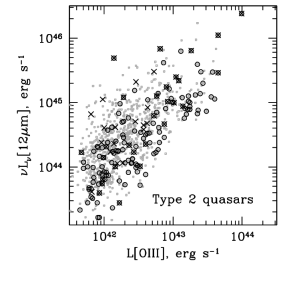
Figure 1.— [OIII] and 12µm luminosities of type 2 quasars with 160µm photometry from Spitzer or Herschel (circles; Section 3) and Spitzer spectroscopy (crosses; Section 4). The background grey points show the parent sample of type 2 quasars (Reyes et al., 2008).

Our second sample is comprised of 115 type 1 quasars at $z\lesssim 0.5$ studied with Spitzer spectroscopy by Shi et al. (2007). Of these, 90 are ultraviolet-excess Palomar-Green (PG; Schmidt & Green 1983; Green et al. 1986) quasars, and the remaining 25 are quasars selected from the Two Micron All Sky Survey (2MASS) with red $R-K$ colors (Cutri et al., 2001; Smith et al., 2002). Thus it is a heterogeneous quasar sample that includes objects with a range of extinction, from $A_{V}\simeq 0$ to $\lesssim 5$ mag (Zakamska et al., 2005), but overall it is dominated by type 1 (broad-line) sources. In the few cases of narrow-line (type 2) classification in the optical, broad emission lines and strong quasar continuum are seen in the near-infrared (Glikman et al., 2012). Hereafter, we refer to these objects collectively as type 1 sources, sometimes making a distinction between ‘blue’ and ‘red’ as necessary, according to whether they are drawn from the PG sample or the 2MASS sample.

Out of 115 type 1 quasars, all but one have complete 4-band photometry from Wide-field Infrared Survey Explorer (WISE; Wright et al. 2010). We calculate rest-frame 12µm mid-infrared luminosities by power-law-interpolating between WISE-3 and WISE-4 bands, and then estimate bolometric luminosities by applying bolometric correction of 8.6 from Richards et al. (2006). Spitzer spectroscopy is available for all 115 objects (Shi et al., 2007). For red type 1 quasars, we collect archival Spitzer photometry (Section 2.2) and for blue type 1 quasars we use recently published Herschel photometry (Section 2.3), so that 114 out of 115 objects have far-infrared photometric data.

The redshifts and mid-infrared luminosity distributions of type 1 and type 2 samples are similar, as shown in Figure 2. For 39 of the 115 type 1 quasars, [OIII] luminosity measurements are available in the catalog of Shen et al. (2011). For this subsample, we find $L_{\rm[OIII]}=10^{42.3\pm 0.6}$ erg s^-1 (average and standard deviation), similar to the range probed by the type 2 sample with follow-up infrared data ($10^{42.5\pm 0.5}$ erg s^-1).

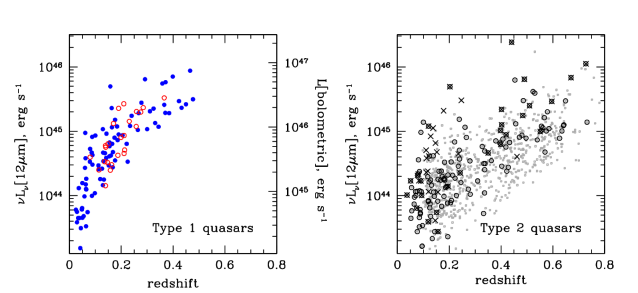
Figure 2.— Redshift and mid-infrared luminosity distributions of both quasar samples discussed in this paper. Left: PG (filled blue circles) and 2MASS (open red circles) type 1 quasars with Spitzer spectroscopy presented by Shi et al. (2007) and Spitzer and Herschel photometry. Right: type 2 quasars with 160µm photometry from Spitzer or Herschel (circles) and Spitzer spectroscopy (crosses) and with parent sample (Reyes et al., 2008) in grey. We estimate the bolometric luminosities of type 1 quasars from their 12µm monochromatic luminosities (right axis of the left panel) using Richards et al. (2006) bolometric correction of 8.6 (which ranges between 7.8 and 9.3 depending on the assumed spectral energy distribution). Type 2 quasars likely have higher bolometric corrections.

Type 2 quasars are redder in the mid-infrared than type 1 quasars (Liu et al., 2013b). Specifically, the infrared power-law index between rest-frame 5 and 12µm luminosities $\beta$ (defined as $\nu L_{\nu}\propto\lambda^{\beta}$) is $-0.05\pm 0.30$ (mean and standard deviation) for type 1 quasars from Shi et al. (2007), whereas for the type 2 quasars from Reyes et al. (2008) catalog it is $\beta=0.78\pm 0.45$. Furthermore, the ratio of 12µm luminosities to $L_{\rm[OIII]}$ is 0.5 dex higher in type 1 quasars than in type 2s at the same emission line luminosity (Zakamska et al. in prep.). Both these factors suggest that 12µm luminosity is not an isotropic measure of quasar luminosity and that type 2 quasars are obscured even at mid-infrared wavelengths. The bolometric corrections of type 2 quasars are therefore likely to be higher than those of type 1 quasars, perhaps by as much as a factor of $\sim 3$ (which would be necessary to reconcile the infrared-to-[OIII] ratios of type 1s and type 2s), but as they remain uncertain we do not show them in Figure 2.

2.2. Far-infrared photometry with Spitzer

Composite spectral energy distribution models (e.g., Polletta et al. 2007; Mullaney et al. 2011; Chen et al. 2015) attempt to decompose emission from active galactic nuclei into a component powered by the black hole and a component powered by star formation in the host galaxy, and to use these measurements to determine the power of both processes. At the heart of these methods is the empirical notion that dust heated by the black hole accretion is warmer than that heated by starlight, and thus a quasar-dominated spectral energy distribution peaks at shorter wavelengths than that of a star-forming galaxy (de Grijp et al., 1987). Therefore, observing longward of thermal peaks maximizes sensitivity to star formation and minimizes contamination by the quasar.

We cross-correlate the 887 type 2 quasars from Reyes et al. (2008) against the Spitzer Heritage Archive and we find 62 distinct sources with nominal coverage at 160µm (the longest available wavelength) by the Multiband Imaging Photometer for Spitzer (MIPS; Rieke et al. 2004), and we download the corresponding 100 distinct Astronomical Observation Requests (AOR). We use filtered (mfilt, mfunc) post basic calibrated data (PBCD) products to perform point-spread function (PSF) photometry. To this end, we generate PSF models using STinyTim (MIPS Instrument Handbook, 2011) and develop an analytic approximation to them using piece-wise Airy functions; a detailed description of the PSF is available in Aniano et al. (2011).

With this in hand, we perform PSF photometry of the First Look Survey, which allows us to calibrate our PSF fitting procedure against the catalog of 160µm sources by Frayer et al. (2006). We find that our measurements are systematically fainter than theirs by 24%, which we attribute to color corrections which they applied and we did not. We take their fluxes to be ‘true’ values and correct the systematic offset using a constant multiplicative factor (analogous to their use of color corrections), after which we find excellent agreement between their fluxes and ours within their stated absolute uncertainty of 25%. In the absence of color information, we cannot tailor our color corrections to a specific target. Having thus calibrated our PSF photometry procedure, we apply it to the MIPS-160 data of type 2 quasars.

Of the 62 sources, 11 have poor enough data quality (covered on the edges of big scans, gaps in coverage overlapping with the source location) that we do not consider them. The 51 sources with acceptable data quality are listed in Table Star formation in quasar hosts and the origin of radio emission in radio-quiet quasars; of these, 12 are detected, both as evaluated by the improvement in reduced $\chi^{2}$ over a continuum-only fit and by visual inspection. Following Frayer et al. (2006), we adopt 25% as the photometric uncertainty. The median value of detected flux is 101 mJy. For the remaining sources we derive upper limits by fitting PSFs at multiple random locations within the field of the object and deriving the standard deviation of the fitted fluxes, which is taken as a 1$\sigma$ limit for point-source detection. In Table Star formation in quasar hosts and the origin of radio emission in radio-quiet quasars, we give 5$\sigma$ upper limits derived using this procedure. The median upper limit is 84 mJy.

We then select all good observations of the 39 non-detected sources by choosing only those with the reported uncertainty in the vicinity of the object of $<0.4$ MJy/sr, which roughly corresponds to a 5$\sigma$ sensitivity for point source detection of 280 mJy. We then make cutouts from these data centered on the known positions of our sources and we stack them using error-weighted averaging. We find a strong ($\sim 10\sigma$) detection in the stacked image, with a PSF flux of 23 mJy, which we take to be an estimate of the mean flux of non-detected sources. We also conduct a null test, in which all images to be stacked are randomly offset by several pixels from the source position. There is no source detection in the null test stack.

The sample of type 2 quasars with archival MIPS-160 data is heterogeneous, as described in Table Star formation in quasar hosts and the origin of radio emission in radio-quiet quasars. 25 objects constitute the full content of our targeted program (GO-3163, PI Strauss); they were selected based on [OIII]$\lambda$5007Å luminosity ($L_{\rm[OIII]}\geq 10^{42.5}$ erg s^-1), tend to be at relatively high redshifts $(z\gtrsim 0.30)$ and show low rates ($<20\%$) of MIPS-160µm detection. Three were observed by other groups because they are powerful radio galaxies with strong enough line emission to make it into the [OIII]-selected sample of Reyes et al. (2008). Five objects at low redshifts were observed by other groups as candidate Ultraluminous Infrared Galaxies (ULIRGs) or type 2 quasars, and these are strongly detected with high fluxes. 18 objects are covered serendipitously by observations of other targets or calibration observations. Thus is it not surprising to have a few bright detections (in particular, nearby objects selected by other observers as ULIRG candidates) supplemented with many objects that are much fainter.

For the 25 objects covered by our program GO-3163, we also have MIPS-70 measurements performed in 2006 (previously unpublished). For MIPS-70, we computed fluxes by aperture photometry using MOPEX with aperture radius of $16^{\prime\prime}$ and applying aperture corrections derived from mosaicked images. The statistical errors were estimated from rms fluctuations of backgrounds. The color correction was applied assuming power-law flux density with the slope of $-1$. Twelve of the objects are detected at $>3\sigma$ level (whereas only four in the same program GO-3163 are detected in MIPS-160). In this paper we use these 12 detected sources to estimate infrared colors of type 2 quasars in Section 3.3, leaving a detailed analysis of the spectral energy distributions for future. The MIPS-24 observations in this program have been superseded by WISE-4 data.

As for the type 1 sample, the majority of blue quasars were observed by Herschel as described in the next section and in Petric et al. (2015). Since Herschel data supersedes MIPS-160 data, we do not rematch the blue quasars to the Spitzer archive. All 25 red type 1 quasars are covered by archival MIPS-160 observations from two programs: 11 objects were observed by PI F. Low as a follow-up of 2MASS-selected quasars, and the remaining 14 objects were observed by PI G. Rieke as a follow-up of the most luminous quasars known at $z<0.3$. We analyze the photometry of these 25 sources in the same way as we do the type 2 sample and include them in Table Star formation in quasar hosts and the origin of radio emission in radio-quiet quasars. 17 objects are detected with a median flux of 139 mJy and for 8 objects we give upper limits with a median value of 114 mJy.

2.3. Far-infrared photometry from Herschel

We proceed to Herschel photometry of type 2 quasars from Reyes et al. (2008). Our Herschel sample is assembled from two programs of pointed observations. In the first one (PI Zakamska), we obtained pointed observations of seven [OIII]-luminous sources ($L_{\rm[OIII]}\geq 10^{43.0}$ erg s^-1, median $L_{\rm[OIII]}=10^{43.2}$ erg s^-1) whose optical line emission was studied in detail by Liu et al. (2013a, b). In the second (PI Ho), we obtained pointed observations of 90 sources roughly matched in redshift, infrared luminosity and [OIII] luminosity to the PG sample (Figure 2) and sampling the full range of [OIII] luminosities ($L_{\rm[OIII]}=10^{41.7-43.4}$ erg s^-1) of the parent sample of Reyes et al. (2008). Similarly deep photometry was obtained in both programs using the Photodetector Array Camera and Spectrometer (PACS) in the mini-scan map mode at 70µm and 160µm and Spectral and Photometric Imaging Receiver (SPIRE) at 250µm. All our targets are assumed to be point sources at Herschel resolution (the full width at half maximum of the point spread function is 12″).

For the smaller program (PI Zakamska), we use Level 2 PACS and SPIRE observations produced by standard pipeline reduction procedures (described in Chapter 7 of the PACS observing manual and in Chapter 5 of SPIRE data handbook). Source confusion is not an issue in PACS bands: at 0.7 mJy (Magnelli et al., 2013), confusion at 160µm is well below our $1\sigma$ sensitivity of 2.5 mJy. We perform aperture photometry in the Herschel Interactive Processing Environment (HIPE) version 10.0 around the optical positions (known to better than 0.1″, with Herschel absolute pointing error of 0.81″, Sánchez-Portal et al. 2014). We use the AnnularSkyAperturePhotometry task within HIPE and apply aperture corrections using the PhotApertureCorrectionPointSource task. We detect all seven sources at 70µm and six of them at 160µm at above 3$\sigma$, with median fluxes of 22 mJy and 16 mJy, respectively. This photometry is presented in Table Star formation in quasar hosts and the origin of radio emission in radio-quiet quasars.

For the SPIRE images, we use an extraction and photometry task in HIPE that implemented the SUSSExtractor algorithm described by Savage & Oliver (2007). We do not detect any sources in the SPIRE bands, where our nominal $1\sigma$ point-source sensitivity is slightly below the confusion limit, 6 mJy at 250µm (Nguyen et al., 2010), and our images are indeed confusion-limited. Extrapolating our measured PACS-160 fluxes to the SPIRE-250 band using $F_{\nu}\propto\nu^{4.5}$ typical of the long-wavelength spectrum of star-forming galaxies (Kirkpatrick et al., 2012), we find that the median flux in SPIRE-250 is expected at the $\sim 3$ mJy level, below the confusion limit, thus the lack of detections is not surprising.

Herschel data for type 2 quasars from the larger program (PI Ho) will be presented in their entirety by Petric et al. (in prep). Here we use exclusively 160µm PACS fluxes from this program obtained using aperture photometry tools in HIPE in a manner similar to that described in Petric et al. (2015). In this Herschel program, 90 objects were observed, 76 of them were detected and for the remaining 14 we set 4$\sigma$ upper limits.

For blue type 1 quasars Herschel photometric data are published in Petric et al. (2015) and we use their 160µm fluxes here. 85 objects were observed, 69 of them were detected and for the remaining 16 we use upper limits from Petric et al. (2015). Out of the remaining five blue type 1s from the sample of Shi et al. (2007), four have 160µm photometry from Spitzer or ISO in the literature (Haas et al., 2000; Shang et al., 2011), and we include them in our analysis.

2.4. Spectroscopic observations

Mid-infrared spectra of galaxies contain a wealth of information on star formation processes and on the nuclear activity, including the emission features of polycyclic aromatic hydrocarbons (PAHs; Allamandola et al. 1989; Roussel et al. 2001; Dale & Helou 2002) and the low-ionization and high-ionization ionic emission lines ([NeVI]$\lambda$7.65µm, [SIV]$\lambda$10.51µm, [NeII]$\lambda$12.81µm, [NeV]$\lambda$14.32µm, [NeIII]$\lambda$15.56µm, Farrah et al. 2007; Inami et al. 2013). Our analysis is based on the Spitzer Space Telescope Infrared Spectrograph (IRS; Houck et al. 2004) low-resolution spectra of quasars of different types. For type 1 blue PG quasars and red 2MASS quasars, we use published spectra and analysis by Shi et al. (2007). As for type 2 quasars, we cross-correlate the type 2 quasar sample (Reyes et al., 2008) against IRS data using Spitzer Heritage Archive.

We find 46 type 2 quasars from Reyes et al. (2008) with IRS spectra of varying quality within 3″ of the optical position. In Table Star formation in quasar hosts and the origin of radio emission in radio-quiet quasars we list type 2 quasars with mid-infrared spectroscopic measurements as well as comments on how these objects were selected for follow-up spectroscopy. The majority were targeted by various groups as type 2 quasar candidates. Ten of them were from our own program (Zakamska et al., 2008) and were selected based on [OIII] luminosity and infrared flux ($L_{\rm[OIII]}>10^{42.6}$ erg s^-1, $F_{\nu}$[8µm]$>1.5$ mJy, $F_{\nu}$[24µm]$>6$ mJy). Other programs selected targets based on X-ray properties and optical or infrared luminosity diagnostics. Thus the sample is a fairly representative subsample of the Reyes et al. (2008) sample of type 2 quasars (Figure 2). Depending on the redshifts of the targets and on which IRS gratings were used for the observations, the wavelength coverage ranges from $\sim$5-13µm in the rest-frame (12 objects) to $\sim$5-25µm (the rest of the sample). Example spectra are shown in Figure 3. There are 28 objects in common between the type 2 sample with IRS spectra and the type 2 sample with 160µm photometric data; these sources are discussed in Section 4.3.2.

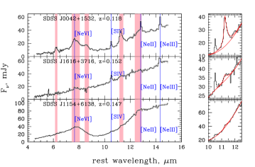
Figure 3.— Example spectra of three type 2 quasars from our sample: from top to bottom, a spectrum with relatively strong PAHs, a power-law-dominated spectrum and a silicate-absorption-dominated spectrum. On the right, we show PAH[11.3µm] fits with fixed shape of the PAH feature taken from Smith et al. (2007) and third order polynomial continuum. Pink shading shows the expected locations of PAH complexes, vertical blue lines show positions of some of the brightest emission lines. The broad absorption feature extending from $\sim 8$µm to $\sim 13$µm in SDSS J1154+6138 is due to silicates.

As the majority of the sources are point-like at Spitzer resolution, we use the enhanced data products described in Chapter 9 of the IRS Instrument Handbook. In a handful of cases where several spectra of the same target are returned by the search engine (perhaps because the IRS coordinates are slightly offset from one another) we combine the spectra into one using error-weighting. We inspect all spectra to make sure that the short- and the long-wavelength (SL and LL) spectra stitch together well in the region of the overlap. Because the LL grating has a larger aperture than the SL one, for extended sources some of the flux may be missed by the SL grating (Brandl et al., 2006); furthermore, even for point sources slight relative mis-alignment of the gratings would result in a greater loss of flux from the SL slit. In 10 cases we apply a multiplicative factor $>$1 to the SL spectrum to bring it into the agreement with the LL spectrum; only in 5 of these cases is the adjustment greater than 10%.

With these spectra in hand, we double-check their absolute flux calibrations. Because we primarily use PAH[11.3µm] fluxes in the analysis which follows, absolute flux calibration around this wavelength is particularly important. We convolve the spectra with the Wide-Field Infrared Survey Explorer (WISE) filter curves from Jarrett et al. (2011), obtain synthetic fluxes in the WISE-3 band (effective wavelength 11.6µm) and compare those with observed WISE-3 fluxes. They show excellent agreement, with the average ratio between synthetic fluxes and observed fluxes of 0.03 dex and the standard deviation among the 46 objects of 0.04 dex. We therefore take 0.05 dex (12%) to be the absolute flux calibration uncertainty for these sources.

To calculate PAH fluxes, we cut out $\lesssim$3µm-wide chunks of the spectrum and model them using a polynomial continuum and Drude profiles with profile shapes and widths taken from Smith et al. (2007). Drude (or damped harmonic oscillator) profiles arise in the Drude theory of conductivity (Bohren & Huffman, 1983) and are found to be very well matched to ultra-violet and infrared opacity curves of small dust particles (Fitzpatrick & Massa, 1986). For PAH complexes, such as those at 11.3µm and at 7.7µm, the relative amplitudes of the components within the complex are fixed to their ratios in the template spectrum of normal star-forming galaxies (Smith et al., 2007). For example, within the 11.3µm complex the amplitude ratio of the 11.23µm and 11.33µm components is fixed to 1.25:1. Depending on the model for the local continuum, from a constant to a cubic polynomial, the number of fit parameters varies from two to five, with the amplitude being the only parameter that describes the intensity of the PAH feature (since the functional shape of the feature remains fixed). Example fits are shown in Figure 3. Overall the 11.3µm and the 6.2µm features are reproduced well, but the quality of fits of the 7.7µm feature is poor. Contributing factors are a strong [NeVI]7.652µm emission line blended with the PAH complex and a poorly anchored continuum, whose shape is complicated by silicate absorption. We therefore do not use the results from the PAH[7.7µm] fits.

The mid-infrared continua of obscured quasars show a wide range of behavior of the silicate feature centered at 9.7µm, from deep absorption to occasional emission (Sturm et al., 2006; Zakamska et al., 2008). We measure the apparent strength of silicate absorption defined as $S[9.7\micron]=-\ln(f_{\rm obs}[9.7\micron]/f_{\rm cont}[9.7\micron])$, where $f_{\rm obs}$ is the observed flux density at 9.7µm and $f_{\rm cont}$ is the estimate of silicate-free continuum obtained by power-law interpolation between $5.3-5.6\micron$ and $13.85-14.15\micron$. Negative values of $S[9.7\micron]$ indicate silicate emission, while positive values indicate absorption, with $S[9.7\micron]\gtrsim 1$ for the 10% most absorbed sources. This method is similar to that used by Spoon et al. (2007), except we do not use a continuum point at 7.7µm even in the cases of weak PAH emission. The apparent strength of Si absorption is closely related to, but not identical to the optical depth of Si dust absorption; depending on the poorly known continuum opacity of the dust at these wavelengths, the actual optical depth is $\simeq(1.2-1.5)\times$ the apparent strength of the Si feature (Zakamska, 2010).

Forbidden lines [NeII]$\lambda$12.81µm, [NeIII]$\lambda$15.56µm, [NeV]$\lambda$14.322µm, [NeVI]$\lambda$7.652µm and [SIV]10.51µm are measured by fitting Gaussian profiles plus an underlying linear continuum. As these lines are not spectrally resolved, their widths $\sigma$ in the observer’s frame are fixed to the order-dependent instrumental resolution tabulated by Smith et al. (2007). We cut out a $3\sigma-$wide piece of spectrum centered on the emission line in question and perform a three-parameter fit, with two parameters describing the continuum and one parameter for the line amplitude. We allow for an 0.03µm variation in the line centroid to account for the wavelength calibration uncertainty (Smith et al., 2007). Because our fits for PAH emission features and forbidden emission lines are linear in all parameters, we use the standard error as the estimate of the standard deviation of the parameter estimate.

In addition to the 46 type 2 quasars with spectra, we use 115 IRS spectra for all type 1 quasars from Shi et al. (2007). As was described in the beginning of Section 2, 90 of these are optically selected blue PG quasars and 25 are near-infrared-selected quasars of varying optical types. The IRS sample was assembled from several dedicated programs and archival search as described by Shi et al. (2007), and their spectra were analyzed in detail using methods similar to ours. In each of the three subsamples (blue type 1 quasars, red type 1 quasars, type 2 quasars) the detection rate of the 11.3µm PAH feature is $\sim$ 50%, and we use upper limits on PAH fluxes in the remaining objects.

2.5. Radio data

We cross-match all objects with spectroscopic or photometric infrared data with the Faint Images of Radio Sky at Twenty cm survey (FIRST; Becker et al. 1995; White et al. 1997) within 3″ of the optical position. FIRST used the Very Large Array to produce a catalog of the radio sky at 1.4 GHz with a resolution of 5″, subarcsec positional accuracy, rms sensitivity of 0.15 mJy and catalog threshold of $\sim 1.0$ mJy for point sources. When a source is covered by the FIRST data but there is no catalog detection, we estimate the flux density upper limit as 5$\times$rms flux density at source position$+0.25$ mJy, with the last term included to correct for the CLEAN bias (White et al., 1997).

In cases of no FIRST coverage (7% of type 2 quasars and 25% of type 1 quasars), we use the NRAO VLA Sky Survey (NVSS; Condon et al. 1998), which is a 1.4 GHz survey covering the entire sky north of $-40\deg$ with a resolution of 45″, positional accuracy of better than 7″, rms sensitivity of $\sim 0.4$ mJy and catalog threshold of $\sim 2.3$ mJy. We match within 15″ of the optical position and in case of non-detections, calculate the upper limit as 5$\times$rms flux density at source position$+0.4$ mJy (White et al., 1997).

Our matching procedure implies that for extended radio sources – a minority of our sample – we are sensitive only to the core fluxes, not to the extended lobes. Inclusion of lobe emission would increase the observed radio luminosities quoted in this paper, but only for a minority of sources. Most objects are point-like at the resolution of FIRST and NVSS (Zakamska et al., 2004), with only 10%-20% sources (both in the type 2 and the type 1 samples) showing integrated fluxes significantly higher than peak fluxes. The radio detection rates are 73% for the type 2 sample with far-infrared photometry, 85% for the type 2 sample with IRS spectroscopy, and 59% for the type 1 sample.

All radio luminosities quoted in this paper are K-corrected to rest-frame 1.4 GHz using equation

$$L_{\rm radio,obs}\equiv\nu L_{\nu}[1.4{\rm GHz}]=4\pi D_{L}^{2}\nu F_{\nu}(1+z)^{-1-\alpha},$$ (1)

where $\nu=1.4$ GHz, $D_{L}$ is the luminosity distance, $F_{\nu}$ is the observed flux density at 1.4GHz, and $\alpha$ is the power-law spectral index defined as $F_{\nu}\propto\nu^{\alpha}$. Radio-quiet quasars at $z\sim 0.5$ are too faint to be detectable by any large radio surveys other than FIRST and NVSS, which have data only at 1.4 GHz, so we cannot measure $\alpha$ from archival data. Values between $-0.5$ and $-1.0$ for the radio-quiet population were suggested in the literature (Barvainis & Antonucci, 1989; Ivezić et al., 2004; Zakamska et al., 2004); unless specified otherwise, we assume $\alpha=-0.7$. For a source at $z=0.5$ with a fixed observed flux density $F_{\nu}$, varying $\alpha$ from -0.7 in its typical range between -0.5 and -1 results in a 10% uncertainty in $L_{\rm radio,obs}$.

3. Star formation rates of quasar hosts from photometry

Dust that produces infrared emission of quasars and star forming galaxies is heated by the radiation from the accretion disk or from young stars. Because of the very high optical depths involved, all incoming radiation at optical and ultraviolet wavelengths is absorbed in a thin layer close to the source of the emission and then thermally reprocessed thereafter. Therefore, it is unlikely that any differences between radiation fields in active and star forming galaxies may be responsible for the noticeable differences in the infrared spectral energy distributions.

Instead, the biggest difference between quasar-heated and star-formation-heated dust is that the latter is distributed over the entire galaxy on $D_{\rm gal}\gtrsim 1$ kpc scales, whereas dust heated by an AGN is concentrated on scales $D_{\rm qso}\lesssim 10$ pc even in luminous objects (Kishimoto et al., 2011). A star-forming galaxy and an active nucleus of similar bolometric luminosities ($L\propto D^{2}T^{4}$) would have different characteristic dust temperatures, $T_{\rm gal}/T_{\rm qso}\sim\sqrt{D_{\rm qso}/D_{\rm gal}}\sim 0.1$. This crude scaling is borne out by far-infrared observations of star-forming galaxies, whose characteristic temperature is $T_{\rm gal}\simeq 25$ K, and of AGN, where the bulk of the thermal emission is produced with $T_{\rm qso}\gg 100$ K (Richards et al., 2006; Kirkpatrick et al., 2012). Beyond this basic temperature distinction, a variety of shapes of the spectral energy distributions can be produced due to the differences in the geometric distribution of dust (compact vs diffuse, spherical vs non-spherical, clumpy vs non-clumpy, etc.), its amount, and its orientation relative to the observer (Pier & Krolik, 1992; Nenkova et al., 2002; Levenson et al., 2007).

Because of the steep decline of the modified black body function at wavelengths greater than those that correspond to the thermal peak, in composite sources with similar contributions from the active nucleus and the star forming host galaxy the mid-infrared emission tends to be dominated by the active nucleus and the far-infrared emission ($\lambda\gtrsim 100\micron$) is dominated by star formation (Hatziminaoglou et al., 2010). But in quasars even the longest wavelength emission probed by Herschel observations can be dominated by emission from hot (presumably quasar-heated) dust (Hony et al., 2011; Sun et al., 2014).

Our approach is therefore to use far-infrared observations to obtain strict upper limits on the quasar hosts’ star formation rates. To minimize the contribution from the quasar – insofar as it is possible – we use the longest wavelength observations available to us. In practice, we use 160µm data either from Spitzer or from Herschel. We then assume that all of the observed far-infrared emission is due to star formation, and calculate the corresponding star formation rates and the expected radio luminosities (Helou et al., 1985; Bell, 2003; Morić et al., 2010). This predicted radio luminosity is an upper limit on the amount of radio emission that can be generated by star formation. We then compare these predictions with the observed radio emission. By using a variety of templates to estimate star formation rates, we ensure that our results are robust to varying the assumed spectral energy distribution of a star-forming galaxy.

Finally, our measurements are predicated on the assumption that the far-infrared fluxes in star-forming galaxies are measuring the instantaneous rates of star formation. This is not always true (Hayward et al., 2014), in that previously formed stars can continue to illuminate left-over dust even after star formation rates have declined. But because this effect results in an over-estimate of star formation rate when using far-infrared fluxes, it is consistent with our upper-limit approach.

The main result of this section is presented in Figure 4 which demonstrates that the radio emission due to star formation in the quasar hosts is inadequate – by almost an order of magnitude – to explain the observed radio emission. Below we describe in detail the steps involved in this comparison and in the cross-checking of this result we performed using a variety of methods.

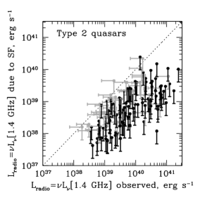
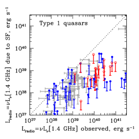
Figure 4.— Left: Results from the far-infrared photometric data from Spitzer and Herschel 160µm observations of type 2 quasars from Reyes et al. (2008). We plot radio luminosity expected due to star formation in the quasar hosts vs the observed radio luminosity. Four points corresponding to radio-loud sources with $L_{\rm radio,obs}>3\times 10^{41}$ erg s^-1 and $L_{\rm radio,SF}<10^{41}$ erg s^-1 are off the scale of the plot to the right. Vertical bars show that all points represent upper limits on host star formation rates (and thus upper limits on the associated expected radio luminosity). Grey points with horizontal error bars denote points that are not detected by FIRST / NVSS, whereas black symbols correspond to radio detections. In the cases where radio emission is detected (74% of the objects), star formation is insufficient to account for the observed radio emission, with the median $\log(L_{\rm radio,obs}/L_{\rm radio,SF})=1.0$. Right: Same calculation for type 1 quasars. Blue points are for PG quasars (predominantly Herschel data from Petric et al. 2015) and red for 2MASS quasars (MIPS-160 data) detected in the radio, and grey points are for radio non-detections. For these objects, the median $\log(L_{\rm radio,obs}/L_{\rm radio,SF})=1.1$. Uncertainties in radio fluxes as less than 15%.

3.1. The infrared-radio correlation of star-forming galaxies

The key to making an accurate comparison between the observed radio luminosity and that predicted from star formation in the host galaxy is a careful calibration between the far-infrared luminosities, star formation rates and radio luminosities due to star formation in star-forming galaxies without an active black hole. The strong correlation between these values is due to massive young stars which dominate the ultraviolet continuum most easily absorbed by interstellar dust, resulting in a ‘calorimetric measure’ of star formation rates (Kennicutt, 1998). The same young stars explode as supernovae, resulting in acceleration of cosmic rays which produce the observed radio emission (Helou et al., 1985).

The tightest correlation is between the total infrared luminosity of star formation (by convention, often integrated between 8 and 1000µm, $L_{\rm 8-1000\micron,SF}\equiv L_{\rm IR,SF}$) and radio luminosity, which we take from Figure 3 of Bell (2003):

$$\log L_{\rm radio,SF}{\rm[erg\,s^{-1}]}=26.4687+1.1054\log(L_{\rm IR,SF}/L_{\odot}).$$ (2)

In this equation and hereafter, the radio luminosity is the monochromatic luminosity at rest-frame 1.4 GHz, $L_{\rm radio}\equiv\nu L_{\nu}$[1.4GHz].

To reassure ourselves that this relationship applies to galaxies with a wide range of star formation rates – including the high star formation rates we confront in infrared-luminous sources discussed in this paper – we double-check this conversion against data for two samples of star-forming galaxies analyzed completely independently from Bell (2003) by several different groups. At low luminosities, we use nearby galaxies from Mullaney et al. (2011). At high luminosities, we use the Great Observatories All-Sky Luminous Infrared Galaxy Survey (GOALS; Armus et al. 2009). In both cases, we take advantage of the 8-1000µm infrared luminosities tabulated by Mullaney et al. (2011) and Armus et al. (2009) and obtain radio luminosities from the NVSS.

Because the GOALS sample may contain active galactic nuclei, we restrict our comparison to those objects that have mid-infrared classifications consistent with pure star formation, by requiring the rest-frame equivalent width (EW) of the polycyclic aromatic hydrocarbon emission at 6.2µm to be above 0.3µm (Stierwalt et al., 2013). Although not a perfect diagnostic, this measure is reasonably well correlated with ionization-line diagnostics of AGN activity (Petric et al., 2011). Furthermore, many GOALS galaxies are found in mergers, and the total infrared luminosities of these sources include all components found within the $\sim 5\arcmin$ beam of the Infrared Astronomical Satellite (Neugebauer et al., 1984) which is significantly larger than the NVSS beam ($\sim 45\arcsec$). Thus, in widely separated mergers the infrared emission could include multiple interacting components, while the radio emission would be coming from only one of them. To make sure we compare fluxes from similar apertures, we further restrict our comparison to objects that are either in single non-interacting hosts or in late-stage mergers (‘N’ and ‘d’ classifications of Stierwalt et al. 2013), excluding pairs and triples at all interaction stages. For these objects, using NVSS fluxes ensures that the total radio emission is taken into account.

Overall we find good agreement between the infrared-radio correlation reported by Bell (2003) and that displayed by these two samples of star-forming galaxies which sample three orders of magnitude in infrared luminosity. Given a measurement of the total infrared luminosity, the standard deviation of the radio luminosity of two samples around the best-fit correlation is 0.16 dex (for Mullaney et al. 2011 galaxies) and 0.24 dex (for GOALS galaxies), which we take to be the practical measure of the uncertainty in the $L_{8-1000\micron}$-radio correlation.

In quasars, the total infrared luminosity may be dominated by the activity in the nucleus, and without many additional assumptions we cannot obtain a measurement of total infrared luminosity due to star formation alone. Thus our challenge is to make the best guess of the upper limit on the star formation rate and on the associated radio emission from just one photometric datapoint at 160µm. To this end we use the calibrations presented by Symeonidis et al. (2008) for star forming galaxies derived from deep MIPS data:

$$\log(L_{\rm IR,SF}/L_{\odot})=1.16+0.92\log(\nu L_{\nu}[70\micron]/L_{\odot});$$ (3)

$$\log(L_{\rm IR,SF}/L_{\odot})=1.49+0.90\log(\nu L_{\nu}[160\micron]/L_{\odot}).$$ (4)

These relationships are well calibrated even in the highly star-forming regime.

Thus our calculation of the expected radio emission due to star formation involves the following steps. We use equations (3)-(4) to convert a far-infrared photometric detection to the total luminosity of star formation, and then we use equation (2) to derive the expected radio luminosity. To verify that the scaling relationships give the correct answer for star forming galaxies, we apply this method to the GOALS sample in Figure 5. We use 160µm photometry from U et al. (2012). Since these authors concentrate on the nearby ($z<0.083$) subsample, we can use equation (4) directly without any need for k-corrections.

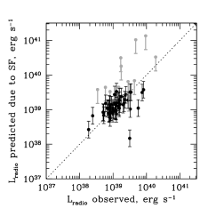
Figure 5.— Comparison between predicted radio emission due to star formation obtained from 160µm fluxes from scaling relationships (4) and (2) and the observed radio emission for GOALS galaxies (Armus et al., 2009; U et al., 2012), most of which are dominated by star formation. Black points show 160µm detections, with 0.24 dex error bars which reflect the conversion of total infrared luminosity to predicted radio due to star formation for GOALS galaxies and grey points show 160µm upper limits. We find excellent agreement between the observed and predicted radio luminosities in galaxies with 160µm detections, with a standard deviation around the 1:1 relationship (dotted line) of 0.18 dex and a mean difference of 0.03 dex. The three most significant outliers below the dotted line all contain active nuclei, which presumably contribute excess radio emission over that associated with star formation alone.

We find an excellent agreement between the observed radio luminosity and that predicted from the 160µm flux via the scaling relationships. Only three points show a significant ($>0.4$ dex) excess of radio emission over that predicted from the 160µm fluxes, and all three turn out to contain luminous active nuclei (MCG-03-34-064 is a Seyfert 1 galaxy, and NGC 5256 and NGC 7674 are Seyfert 2s, Petric et al. 2011) which likely contribute radio emission in excess of that due to star formation in the host. Excluding these three sources, we find that the median / average ratio of the observed-to-predicted flux is 0.01 / 0.03 dex, and the standard deviation around the 1:1 relationship is 0.18 dex. Therefore, we assume that the typical uncertainty in our method of predicting radio emission due to star formation from 160µm band fluxes is about 0.2 dex, which is the combination of the standard deviation around the correlation and the typical photometric error of 160µm observations (20-25%, or $<0.1$ dex). Encouraged by such excellent agreement between predicted and observed radio fluxes in luminous star-forming galaxies, we apply the same method to quasars in the next section.

3.2. Radio emission in quasars is not due to star formation

We use the observed 160µm fluxes (or upper limits) of the quasars in our samples to derive the upper limit on their total infrared luminosity due to star formation using equations (3)-(4). Because the relations are given at rest-frame 70µm and 160µm, and the spectral slopes of our targets are unknown, instead of performing k-corrections on the data we linearly interpolate the slopes and the normalizations of equations (3)-(4) between rest-frame 70µm and 160µm depending on the redshift of each target, thereby establishing a relation between monochromatic luminosity and the total luminosity of star formation at rest-frame wavelength of 160µm/$(1+z)$. We then use equation (2) to derive an upper limit on the radio emission due to star formation and compare with the observed amount.

The results for both type 1 and type 2 quasar samples are shown in Figure 4. Unlike GOALS galaxies in Figure 5, almost all quasars in our sample show significantly higher radio luminosities than those expected from star formation (and furthermore the predicted radio emission is a strict upper limit on the star formation contribution, as reflected in the one-sided error bars, as not all of the 160µm continuum is due to star formation). Among the quasars which have strong detections in the radio, the median ratio between observed radio luminosity and that expected from star formation is an order of magnitude: $\log(L_{\rm radio,obs}/L_{\rm radio,SF})=1.1$ for type 1 quasars and $1.0$ for type 2s. The standard deviation of this ratio is 0.7 dex for type 2 quasars and 1.1 dex for type 1s, though in the latter case the ratio is not log-normally distributed and the standard deviation is artificially inflated by eight radio-loud sources with $L_{\rm radio}\geq 10^{41}$ erg s^-1. Removing these, we find a standard deviation of 0.7 dex for type 1s as well. In any case, the standard deviation is much greater than the $\sim$ 0.2 dex standard deviation in the calibrations of star formation rates in star-forming galaxies and the $\sim 0.1$ dex 160µm flux uncertainty for detections.

Our main conclusion is that the star formation in quasar hosts falls short of explaining the observed radio emission in quasars by about an order of magnitude. This is consistent with the study by Harrison et al. (2014) who found, using the spectral energy decomposition methods, that the observed radio luminosities were in all cases well above the calculated star formation component in their sample. Quasars in their sample are somewhat less luminous than ours, so the effect is likely more pronounced in our case: at the same star formation rate (Stanley et al., 2015), an increase in the quasar contribution would make the radio/160µm ratio more discrepant from that measured in star forming galaxies.

It is more difficult to draw conclusions from the radio non-detections in the FIRST and / or NVSS surveys (shown as grey points in Figure 4), because in this case both the predicted radio luminosity due to star formation and the observed luminosity are only available as upper limits. Nonetheless, these objects do not alter our main conclusion. We have stacked the FIRST images of the non-detected sources in Figure 4, left, and obtained a strong point source detection with a mean peak flux of 0.4 mJy/beam. This estimate is in excellent agreement with our previous finding in Stripe 82 (Zakamska & Greene, 2014), where we were able to detect all FIRST-undetected sources in a more sensitive survey (Hodge et al., 2011) with fluxes about a factor of 2 below the limit of the FIRST survey ($\sim 1$ mJy). If in Figure 4 all sources without radio detections have typical fluxes of 0.4 mJy, then we can again calculate the excess of observed radio emission over the upper limit on radio emission from star formation, which we find to be $\log(L_{\rm radio,obs}/L_{\rm radio,SF})=0.59$ for type 1 quasars and $=0.74$ for type 2s.

To make sure that our results are robust to changes in the spectral energy distribution of star formation, we use several star formation templates available in the literature to recalculate the total infrared luminosity of star formation. We use seven templates, five from nearby star forming galaxies by Mullaney et al. (2011) and two from $z=1-2$ star forming galaxies by Kirkpatrick et al. (2012). We scale the templates (properly adjusted for redshift) to reproduce the observed 160µm fluxes of our sources, with one fitting parameter – the overall luminosity of the template. For each template, we obtain the total infrared luminosity $L_{\rm IR,SF}$ due to star formation by integrating the scaled template between 8 and 1000µm, and of the seven results we pick the highest one, in keeping with the strict upper limits approach, which we convert to the expected radio luminosity (Bell, 2003). The results are qualitatively similar to those obtained via scaling relations from Symeonidis et al. (2008) and shown in Figure 4, though the star formation rates obtained using the template method are systematically higher by about 0.2 dex. The reason for this is that we pick the most conservative template – the one that gives us the highest star formation rate at a given 160µm flux. Even with this method, the observed radio luminosities of quasars are in excess of those predicted from star formation, with $\log(L_{\rm radio,obs}/L_{\rm radio,SF})=0.6$.

3.3. Contribution of the active nucleus to the far-infrared flux

Figure 6 shows the comparison between the spectral energy distribution of one of our obscured quasars and the star-forming galaxy templates. The spectral energy distribution is assembled from photometric data from SDSS, WISE and Herschel, and the seven star formation templates (Mullaney et al., 2011; Kirkpatrick et al., 2012) are scaled to match the 160µm observation. The spectral energy distribution of this object peaks at significantly shorter wavelengths (between 10 and 20µm) than that of any of the star formation templates (between 50 and 150µm); this is typical of our targets.

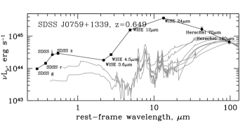
Figure 6.— The spectral energy distribution of one of the obscured quasars from Reyes et al. (2008) and Liu et al. (2013a). Seven star-formation templates from Kirkpatrick et al. (2012) and Mullaney et al. (2011) are scaled to match the longest wavelength point. While it is clear that the overall spectral energy distribution of the object is inconsistent with any of the star formation templates (with excess emission at mid-infrared wavelengths likely due to quasar-heated dust), we can use the longest wavelength detection to place strict upper limits on the star formation rate in the quasar host galaxy.

In Figure 7, left, we show infrared colors of our sources (black) compared with those of template star-forming galaxies (red) which are placed at the same redshift range as our targets ($z=0.24-0.73$). Quasars from our sample have noticeably warmer / bluer colors in the infrared than do star-forming galaxies. In principle, if we knew the spectral energy distribution of a ‘pure quasar’ (i.e., a component that included the circumnuclear obscuring material where heating is dominated by the nucleus but excluded the larger host galaxy where heating is dominated by the stars) then from the observed colors of our objects we could determine the fractional contribution of the AGN and the host galaxy to each spectral energy distribution.

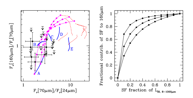
Figure 7.— Left: Infrared colors of type 2 quasars: black points and upper limits for Herschel and Spitzer observations of type 2 quasars detected at 70µm in our targeted deep Spitzer observations. Dotted red lines show infrared colors of seven star formation templates (Mullaney et al., 2011; Kirkpatrick et al., 2012) placed at $z=0.24-0.73$. Solid blue lines show the same for six obscured quasar templates: A – ‘Hot DOGs’ (Tsai et al., 2015), B – ‘featureless AGN’ (Kirkpatrick et al., 2012) and ‘obscuring torus’ (Polletta et al., 2007), C – ‘type 2 quasar’ (Polletta et al., 2007), D – ‘silicate AGN’ (Kirkpatrick et al., 2012) and E – Mrk231 (Polletta et al., 2007). Magenta curves with dots show the color locus of the linear combinations, for three different redshifts, of a star formation template with the HotDOG template. Dots mark 0, 10%, 20%, etc. contribution to the total 8-1000µm infrared luminosity. All model colors include convolution of the templates with filter curves. Right: For three different redshifts (from top to bottom, $z=0.24$, 0.49 and 0.73 – the bracketing redshifts of our sample, plus one value in the middle of the range), the relationship between the SF contribution to the apparent 160µm flux as a function of its contribution to the bolometric luminosity. Even when star formation contributes only 20% to the bolometric luminosity, over half of the apparent 160µm flux is due to star formation for the redshifts of our sample.

To this end, we collect obscured AGN templates from the literature, including three from SWIRE (Polletta et al., 2007): Mrk231 which has a power-law-like spectral energy distribution in the mid-infrared, ‘obscuring torus’ which has a steep cutoff both at short and long wavelengths, and ‘type 2 quasar’, which is obtained by heavy reddening of a type 1 quasar spectral energy distribution. These are supplemented by two more templates from Kirkpatrick et al. (2012): ‘featureless AGN’ that do not show silicate absorption, and ‘silicate AGN’ which do. Finally, we also include the median spectral energy distribution of hot dust-obscured galaxies (HotDOGs) from Tsai et al. (2015). The observations of these extremely luminous high-redshift obscured quasar candidates cover rest-frame wavelengths $\lesssim 100$µm, so in order to compute the 160µm/70µm colors we extrapolate the HotDOG template using a modified Rayleigh-Jeans spectrum with $\beta=1.5$ (Kirkpatrick et al., 2012) beyond 100µm. The model colors of AGN templates at $z=0.24-0.73$ are shown with blue lines in Figure 7.

Intriguingly, half of the AGN templates (C – ‘type 2 quasar’, D – ‘silicate AGN’, and E – Mrk231) are redder / colder than the observed colors of type 2 quasars. It is likely that a significant fraction of the total luminosity of these templates is due to the host galaxy instead of the active nucleus, so their colors are between those of the type 2 quasars in our sample and those of the star forming galaxies. ‘Featureless AGN’ and ‘torus’ templates (they have similar colors; marked B) and ‘HotDOGs’ (marked A) have colors that are much closer to those observed in our sample.

The magenta curves mark a linear combination of one of the star formation templates with the HotDOG template, going from 100% of the 8–1000µm luminosity dominated by star formation to 100% dominated by the HotDOG template. The colors of our type 2 quasars are roughly consistent with such linear combinations if the quasar contributes at least half of $L_{\rm IR,8-1000\mu m}$. Thus the observed infrared colors of type 2 quasars suggest that the bolometric luminosities of our objects are likely dominated by the quasar, not star formation in the host galaxy.

However, because the spectral energy distribution of the quasar template declines so steeply beyond the peak, even a small fractional contribution of star formation is sufficient to dominate the observed 160µm flux, as shown in Figure 7, right. As little as 20% contribution of star formation to the total infrared luminosity $L_{\rm IR,8-1000\mu m}$ is sufficient for it to contribute more than 50% of the 160µm flux at the redshifts of our sample. The lower the redshift, the longer is the rest wavelength probed by the 160µm observations, and the smaller the contribution of star formation required to dominate at that wavelength.

Unfortunately, these calculations do not allow us to unambiguously decompose the infrared spectral energy distribution of our sources into a quasar and star formation component, and to turn our upper limits on star formation rates into actual measurements of star formation rates. The primary reason is that the decomposition is sensitive to the assumed template for the quasar contribution, which is clear from the diversity of colors of AGN templates in Figure 7, left. A slight shift of the peak of the AGN template to longer wavelengths results in a larger contribution of the AGN to the 160µm flux and to a smaller required contribution of star formation. The AGN templates are in turn sensitive to the geometry of the obscuring material (smooth vs clumpy, geometrically thin vs geometrically thick) and the relative orientation of the observer to the obscuring structure (Pier & Krolik, 1992; Nenkova et al., 2002).

Wylezalek et al. (2015) conduct detailed spectral energy distribution decomposition of a subsample of 20 type 2 quasars from Reyes et al. (2008) with HST observations most of which are also presented in this paper. The average and the standard deviation of the luminosities of the 20 objects are $L_{\rm[OIII]}=10^{43.1\pm 0.4}$ erg s^-1 and $\nu L_{\nu}$[12µm]$=10^{45.0\pm 0.5}$ erg s^-1, so they represent the luminous end of the objects probed in this paper. Spectral energy distribution fits with CIGALE (Noll et al., 2009) and DecompIR (Mullaney et al., 2011) suggest that in this subsample, the bolometric luminosities are dominated by the AGN (derived AGN fractions are $0.7\pm 0.2$ and $0.8\pm 0.15$ with the two methods, respectively). Nonetheless the median contribution of star formation to the observed 160µm flux is 91%, and the star formation rates derived by Wylezalek et al. (2015) are therefore similar to those we present here as upper limits. These conclusions are in agreement with our analysis based on far-infrared colors. While we continue treating our 160µm-derived star formation rates as upper limits, we keep in mind that they are likely close to the actual star formation rates, even though the bolometric luminosities of our sources are dominated by the quasar.

3.4. Star formation rates of quasar hosts

We compare the upper limits on star formation rates among the different subsamples of quasars discussed in this paper in Figure 8. To convert from infrared luminosities of star formation to star formation rates, we use the calibration from Bell (2003) which is slight modification of that of Kennicutt (1998) and assumes Salpeter initial mass function. In this section we make a distinction between radio-quiet and radio-loud AGN by applying a simple luminosity cut $\nu L_{\nu}[1.4{\rm GHz}]=10^{41}$ erg s^-1 (Zakamska et al., 2004). All sources (except one) with radio luminosities above this cutoff are detected in FIRST / NVSS, so we do not have to worry about upper limits on radio detections in potentially radio-loud sources. Of the 186 type 1 and type 2 quasars with Herschel data, twelve are radio-loud by this criterion.

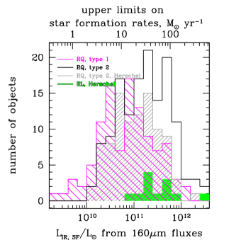
Figure 8.— Distributions of upper limits on infrared luminosities of star formation as derived from 160µm fluxes. For radio-quiet type 1 quasars (magenta, sparsely shaded), the median (average) and the standard deviation are $\log(L_{\rm IR,SF,upper}/L_{\odot})=10.90(10.86)\pm 0.58$, corresponding to the median upper limit on star formation rate of 11.3$M_{\odot}$ yr^-1. Just for the blue type 1 quasars with deep Herschel observations (Petric et al., 2015), we find $\log(L_{\rm IR,SF,upper}/L_{\odot})=10.67(10.72)\pm 0.57$ and 6.3$M_{\odot}$ yr^-1. For radio-quiet type 2 quasars (solid black), $\log(L_{\rm IR,SF,upper}/L_{\odot})=11.24(11.22)\pm 0.54$. Excluding shallow Spitzer observations which include a lot of 160µm non-detections and using only Herschel observations (grey, densely shaded), we find $\log(L_{\rm IR,SF,upper}/L_{\odot})=11.03(11.04)\pm 0.47$, corresponding to median upper limit on star formation rate of 18.1$M_{\odot}$ yr^-1. Type 1 and type 2 radio-loud sources (green, solid fill) with Herschel observations nominally show $\log(L_{\rm IR,SF,upper}/L_{\odot})=11.42(11.52)\pm 0.52$, but their 160µm fluxes can be boosted by synchrotron emission and thus are unreliable measures of star formation.

The first striking result is that the nominal star formation rates are higher in radio-quiet type 2 quasars than in radio-quiet type 1s. Part of this is due to the heterogeneity of our sample: a third of the type 2 quasar sample was observed with Spitzer-160, and these data have shallower observations and higher confusion limits than Herschel-160. As a result, 39 out of 51 type 2 quasars observed with Spitzer-160 are not detected. To make a better-matched comparison between the two samples, we consider only type 2 quasars observed with Herschel-160, the majority of which are detected. These objects still show appreciably higher star formation rates (or rather, upper limits on star formation rates) than type 1s with similarly deep Herschel observations and similar intrinsic luminosities and redshifts. Specifically, the median upper limits on star formation rate derived for hosts of blue type 1 quasars is 6$M_{\odot}$ yr^-1, whereas that of type 2 quasar hosts is 18$M_{\odot}$ yr^-1. (The nominal median upper limit on star formation in red type 1 quasars is even higher, 32$M_{\odot}$ yr^-1, but it is based on shallower MIPS-160 observations, with a third of the sample undetected.) As we discuss in Section 3.3, even though our method technically only allows us to place an upper limit on the star formation rate, the actual values are likely close to the derived upper limits ($\sim 90\%$), so in the following discussion we make the assumption that these star formation upper limits are representative of the actual star formation rates.

It is now well-established that star formation rates in obscured quasars are higher than those in unobscured ones (Kim et al., 2006; Zakamska et al., 2008; Hiner et al., 2009; Chen et al., 2015). This result appears to hold whether star formation is calculated from photometric or spectroscopic indicators. This conclusion is not well-explained by the classical orientation-based unification model, in which type 1 and type 2 quasars should occupy similar host galaxies. The difference in host star formation rates may be due to evolutionary effects: this observation could represent direct evidence that type 2 quasars are more likely to be found in dust-enshrouded environments characteristic of an ongoing starburst (Chen et al., 2015), as suggested by many models of galaxy formation (Sanders et al., 1988; Hopkins et al., 2006).

An alternative explanation for a higher star formation rates in hosts of type 2 quasars is that the selection of these objects is biased toward gas-rich galaxies. It is usually assumed that AGN obscuration happens on circumnuclear scales ($\ll 1$ kpc), and it is not clear whether AGN obscuration is directly connected with the geometry of the host galaxy. In type 2 quasars, which occupy predominantly elliptical hosts, no clear relationship emerges between the presence or absence of the galactic disk and obscuration and their relative orientation (Zakamska et al., 2006, 2008). However, in less luminous type 2 AGN there are indications that at least some of the obscuration is occurring on the galactic scales by the gas and dust in the galaxy disk (Lacy et al., 2007; Lagos et al., 2011). If this is a typical situation in type 2 quasars, then they would be preferentially found in more gas-rich and by extension more star-forming galaxies than type 1s.

Finally, it is possible that type 1 and type 2 quasars discussed in this paper have different bolometric luminosities. While they have similar values of $\nu L_{\nu}$[12µm], this measure could underestimate the luminosities of type 2 quasars which show evidence for obscuration even at mid-infrared wavelengths (Zakamska et al., 2008; Liu et al., 2013b). Therefore, if the type 2s are significantly more luminous than the type 1s, and if the host star formation rate increases with quasar luminosity, then the observed difference in the host star formation rates may be due to the intrinsic differences between the two samples, but this scenario is unlikely given the very flat relationship between the AGN luminosity and the host star formation rates (Stanley et al., 2015). Another possibility is that intrinsically more luminous type 2s (with apparent mid-infrared luminosities similar to those of type 1s) dominate their 160µm fluxes, resulting in higher measured nominal star formation rates, but that is also unlikely in light of the spectral energy decomposition results by Wylezalek et al. (2015) who find that 91% of 160µm emission is due to star formation even in the luminous quasars as discussed in the previous section.

Far-infrared star formation indicators are dominated by obscured star formation and may therefore miss unobscured star formation, which is normally estimated from the ultra-violet luminosities. Ultra-violet measures of star formation are extremely difficult to obtain in type 1 quasars, where the quasar in the nucleus of the galaxy makes identification of circumnuclear star formation all but impossible. Off-nuclear stellar populations, when measured with proper accounting for possible quasar light scattered off the interstellar medium into the observer’s line of sight, tend to show post-starburst features (Canalizo & Stockton, 2013) rather than active star formation. In type 2 quasars, despite nuclear obscuration, ultra-violet emission is dominated by quasar scattered light (Zakamska et al., 2005, 2006; Obied et al., 2015). When this contribution is accounted for, the median ultra-violet rates of star formation in type 2 quasar hosts are $\lesssim 3M_{\odot}$ yr^-1 (Obied et al., 2015), about an order of magnitude lower than those derived from far-infrared luminosities. This is in line with the typical balance between obscured and unobscured star formation found at $z<1$ (Burgarella et al., 2013). Therefore, we conclude that unobscured star formation is unlikely to affect our results.

Another result apparent from Figure 8 is that the nominal upper limits on star formation rates of radio-loud quasars appear to be higher than those of radio-quiet quasars, which is contrary to many previous studies demonstrating that of all types of AGN, these objects are associated with the lowest rates of star formation (Shi et al., 2007; Dicken et al., 2012, 2014). The reason for this discrepancy is that the 160µm fluxes of these objects can be boosted by the synchrotron emission associated with the jet, not by the star formation in the host, particularly in type 1 quasars (four out of seven radio-loud objects) where jet emission might be expected to be beamed. As an example, we take a fiducial radio-loud quasar at $z=0.33$ with $\nu L_{\nu}$[1.4GHz]$=10^{43}$ erg s^-1 and spectral index of synchrotron emission of $\alpha=-0.5$ ($F_{\nu}\propto\nu^{\alpha}$). Such object would appear as a 2.3 Jy radio source at 1.4 GHz, and if its synchrotron spectrum continues all the way to the wavelengths of our far-infrared observations then its 160µm flux due to the jet would be 61 mJy. With our one-band observations, we would calculate a star formation rate of 41 $M_{\odot}$ yr^-1. The exact contribution of synchrotron emission to the 160µm flux depends sensitively on the spectral index and on whether the synchrotron spectrum continues all the way to these high frequencies. We conclude that upper limits on star formation rates derived from 160µm data are not very meaningful for radio-loud objects; their star formation rates are likely lower than those reported in Figure 8.

4. Star formation rates of quasar hosts from spectroscopy

In this section we continue investigating star formation rates in quasar host galaxies (and the resulting radio emission), but now using mid-infrared spectroscopic data. We use polycyclic aromatic hydrocarbon features and low-ionization emission lines as potential star formation diagnostics.

4.1. Calibration of PAHs as star formation diagnostics

Polycyclic aromatic hydrocarbon (PAH) emission dominates mid-infrared spectra of star-forming and starburst galaxies and is typically seen as a star-formation indicator (Allamandola et al., 1989; Genzel et al., 1998; Roussel et al., 2001; Peeters et al., 2004; Kennicutt et al., 2009). Various studies have presented calibrations between PAH luminosities and infrared luminosities of star formation or star formation rates (Brandl et al., 2006; Farrah et al., 2007; Shi et al., 2007; Hernán-Caballero et al., 2009; Feltre et al., 2013), but often either the PAH luminosities or the infrared luminosities or the star formation rates are not measured exactly the same way as what we do here, resulting in significant systematic uncertainties. Most notably, some authors use broad-band 8µm fluxes (Roussel et al., 2001; Kennicutt et al., 2009) which likely overestimate the amount of PAH[7.7µm] emission. Others (e.g., Brandl et al. 2006; Hernán-Caballero et al. 2009) measure PAH luminosities spectroscopically by subtracting an interpolated continuum, which likely results in an underestimate of the PAH fluxes since Drude-like PAH profiles (Smith et al., 2007) have significant flux in the wings. For example, for the 6.2µm feature in ultraluminous infrared galaxies (Hill & Zakamska, 2014) we calculate the PAH flux using the Drude-fitting method, as well as by subtracting a linear continuum interpolated between 5.95µm and 6.55µm, and we find that the former is a factor of 2 higher than the latter.

Of the PAH / star formation calibrations presented in the literature, the one that utilizes the measures closest to ours is presented by Shi et al. (2007). These authors calculate PAH luminosities by fitting Drude profiles to the PAH features, similarly to our procedure, and they find an appropriate star formation template with the same PAH luminosity to calculate the star formation luminosity between 8 and 1000 µm. Their final conversion between PAH[11.3µm] and $L_{\rm IR,SF}$ is well described by

$$\log({\rm PAH[11.3\micron]}/L_{\odot})=-0.7842+0.8759\log(L_{\rm IR,SF}/L_{\odot}).$$ (5)

This calibration can then be supplemented by the IR-to-radio correlation from Bell (2003) listed in equation (2) to obtain a direct relationship between PAH luminosities and radio emission due to star formation:

$$\log L_{\rm radio,SF}{\rm[erg\,s^{-1}]}=27.4584+1.2620\log({\rm PAH[11.3\micron]}/L_{\odot}).$$ (6)

The infrared luminosities due to star formation can be converted to star formation rates (Bell, 2003).

To double-check calibrations (5)-(6), we use nearby star-forming galaxies from Brandl et al. (2006) who tabulated $L_{\rm IR,SF}$ values measured from the Infrared Astronomical Satellite (IRAS; Neugebauer et al. 1984) data. Of the 22 objects presented in their paper, we exclude four with the optical signature of an active nucleus. For the remaining 18, we download the reduced spectra from the Spitzer-ATLAS database (Hernán-Caballero & Hatziminaoglou, 2011), convolve them with IRAS-12µm and IRAS-25µm filter curves from Dopita et al. (2005) to calculate synthetic IRAS fluxes and compare them with those observed. We then augment the spectra by a factor necessary to match the synthetic fluxes to the observed fluxes and use the resulting flux-calibrated spectra to measure PAH luminosities using our Drude-fitting methods. We also obtain the highest listed 1.4 GHz radio fluxes for these galaxies from the NASA/IPAC Extragalactic Database. We assume that any major flux discrepancies between the listed 1.4 GHz measurements are due to varying resolutions of the radio data; for these nearby sources, we prefer the lowest resolution, highest flux observations which are more likely to capture extended radio flux.

On the high-luminosity end, we use a subsample of GOALS galaxies from Stierwalt et al. (2014) dominated by star formation (EW of PAH[6.2µm] $>0.3$µm) and hosted by single or late-stage merger hosts (Stierwalt et al., 2013), as was described in Section 3.1. We further restrict our analysis to objects with silicate absorption strength $<1.1$, to avoid any biases in PAH measurements due to our approach of not correcting PAH fluxes for extinction. Although Stierwalt et al. (2013) present PAH flux measurements, we have found that even minor differences between their and our fitting procedures result in a noticeable systematic offset in PAH/$L_{\rm IR,SF}$ and PAH ratios. Therefore, we re-measure PAH features in these objects using exactly the same tools as those used for type 1 and type 2 quasars. We download the IRS enhanced data products from the Spitzer Heritage Archive, stitch together the SL and LL orders, flux-calibrate using IRAS-12µm and IRAS-25µm fluxes and measure PAHs using our Drude-fitting methods. The radio fluxes of these sources are available in U et al. (2012) and in NVSS. Flux calibration of Brandl et al. (2006) and Stierwalt et al. (2014) spectra against IRAS data is necessary only because some of these objects are so nearby that they are extended beyond the IRS slits. For type 2 quasar spectra, most of which appear as point sources to Spitzer, the default flux calibration provided for the enhanced data products of IRS is in excellent agreement with Spitzer and WISE photometry, and the flux calibration step is unnecessary.

As seen in Figure 9, we find good agreement between the scaling relationships (5) and (6) and the actual measurements in these two samples of star-forming galaxies. Given a measurement of PAH[11.3µm], our adopted calibrations (5) and (6) predict the total infrared and radio luminosities for star-forming galaxies with a standard deviations of $\lesssim 0.3$ dex. Thus the PAH vs star formation conversion appears to have somewhat higher intrinsic spread than the conversion between 160µm flux and $L_{\rm IR,SF}$ and $L_{\rm radio,SF}$, which has a standard deviation of $\lesssim 0.2$ dex. Much of this spread likely reflects the intrinsic dispersion of galaxy properties, as the PAH features are strongly detected in all sources, the quality of the data are high, and PAH measurement uncertainties are only a few per cent for this sample.

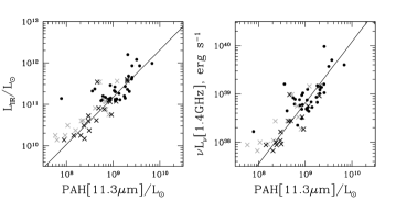
Figure 9.— Double-checking the PAH vs infrared and radio correlations for star-forming galaxies. The solid lines show our adopted calibrations (5) and (6). Crosses show star-forming galaxies from Brandl et al. (2006), in black for results obtained using IRAS-12 for bolometric flux calibration and in grey using IRAS-25. Circles show the star-forming subsample of the GOALS galaxies from Stierwalt et al. (2014). Star-forming galaxies of low and high luminosities show a good agreement with our adopted calibrations, with standard deviations $\lesssim 0.3$ dex.

4.2. PAH measurements of star formation in quasar hosts

As the sources in our sample are quasars with $L_{\rm bol}\gtrsim 10^{45}$ erg s^-1, their continuum emission in the mid-infrared is dominated by the thermal emission of quasar-heated dust, with PAH features sometimes visible on top. In this Section, we start by using the 11.3µm PAH feature exclusively and in Section 4.3 we discuss the reliability of this measure. In Figure 10, left, we show the predicted radio luminosity due to star formation for type 1 quasars analyzed by Shi et al. (2007), and in the right panel we show the same for type 2 quasars.

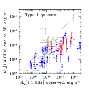
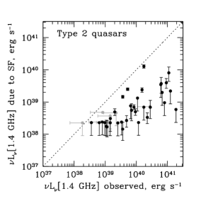
Figure 10.— Results from PAH-based measures of star formation. Left: Radio luminosities expected from star formation and the observed radio luminosities for PG (solid blue circles) and 2MASS (open red circles) quasars from the sample of Shi et al. (2007). Objects not detected in the radio are shown in grey. Right: same for the type 2 quasars from Reyes et al. (2008). The majority of all quasars lie below the 1:1 dashed line, indicating that star formation in quasar host galaxies is insufficient to account for the observed radio emission from quasars, by 1.1-1.3 dex on average.

With the exception of a handful of problematic objects, our task for the Shi et al. (2007) sample is straightforward: we take their measured PAH-derived total luminosities of star formation, convert them to the expected radio luminosity of star formation (eq. 2) and compare with the observed values. We use most of their $L_{\rm IR,SF}$ values, with the following exceptions. We add an upper limit to star formation for PG 0003+158, where we use their upper limit on PAH[11.3µm]. Furthermore, for 2MASS J130700.66+233805.0 and 2MASS J145331.51+135358.7 we do not use their PAH[7.7µm] measurements which are overestimated due to unmodeled ice absorption and instead use their PAH[11.3µm] measurements; this results in a decrease of the calculated $L_{\rm IR,SF}$ for the former object. For type 2 quasars, we use our own PAH[11.3µm] measurements and convert them to the expected radio emission using equation (6).

Figure 10 makes it clear that if PAH[11.3µm] is a good measure of the host galaxies’ star formation rates, then in all quasar samples (blue type 1s, red 2MASS-selected quasars and obscured type 2s) the observed radio emission is well in excess of that expected from the star formation, which is consistent with the results we obtained from photometric measures of star formation in Section 3.2. The median / mean / sample standard deviation ratio of the observed radio emission to that predicted from star formation is 1.1 dex / 1.2 dex $\pm$ 0.9 dex for quasars in the left panel and 1.1 dex / 1.3 dex $\pm$ 1.1 dex for quasars in the right panel (only objects with radio detections were taken into account).

PAHs are detected in half of each subsample – blue type 1s, red type 1s and type 2s. Among the detections, the median star formation rates follow the trend seen in photometric data (lower star formation rates in the blue type 1 subsample than in the other two): 6.7, 26 and 29 $M_{\odot}$ yr^-1, correspondingly. Based on the same dataset, it was pointed out by Shi et al. (2007) that red type 1 quasars occupy more actively star-forming hosts than blue type 1s. We convert non-detections to upper limits on star formation rates, but in some cases the quality of the data make them not very constraining, and the median upper limits are 35, 64 and 17 $M_{\odot}$ yr^-1.

4.3. Issues with PAH measures of star formation

4.3.1 PAHs and dust obscuration

It is not clear to what extent PAH emission is affected by intervening dust absorption. Zakamska (2010) showed that in star-forming ultraluminous infrared galaxies, ratios of PAH complexes at different wavelengths are correlated with the strength of the silicate absorption feature, in a manner consistent with PAH-emitting regions being affected by an amount of obscuration similar to (though somewhat smaller than) that affecting the mid-infrared continuum; this possibility was also pointed out by Brandl et al. (2006) and Imanishi et al. (2007). But this trend is not borne out in a large sample of lower-luminosity GOALS galaxies (Stierwalt et al., 2014). Perhaps only the most luminous, most compact starbursts follow a relatively simple geometry in which both the PAH-emitting regions and the thermal-continuum-emitting regions are enshrouded in similar amounts of cold absorbing gas, whereas in more modest star-forming environments the different components are mixed with one another. Therefore, it remains unclear whether PAH emission is affected by absorption, and any absorption correction would be rather uncertain.

Because type 2 quasars show weak silicate absorption (Zakamska et al., 2008), any putative absorption corrections to PAH fluxes are relatively minor: in 90% of our sample, the peak absorption strength is $S[9.7\micron]<1$, so the optical depth at 11.3µm is less than 0.6 and the correction to PAH flux would be less than 30%, with a median of 8%. But more importantly, in type 2 quasars most of the mid-infrared continuum is due to the quasar-heated dust, and therefore the strength of silicate absorption reflects the geometry of this circumnuclear component. Correcting PAH emission which is likely produced in different spatial regions using this value of silicate absorption appears meaningless, so we do not attempt it.

If star formation in quasar hosts is extremely obscured and if PAH-emitting regions are buried inside optically thick layers of dust, then our methods would underestimate PAH emission, and thus the star formation rate and the expected radio emission. In order for such absorption to completely account for a 1.2 dex offset between the observed and the predicted radio emission, we would need an optical depth of 2.8 at the wavelength of the 11.3µm feature, which corresponds to the strength of the silicate absorption of about $S[9.7\micron]\simeq 4$. Only 6% of ultraluminous infrared galaxies have an apparent absorption strength above 3 (Zakamska, 2010), so such high average values of extinction toward PAH-emitting regions are implausible. Therefore, it is unlikely that using the PAH method we underestimate the star formation rates in quasar hosts by the amount necessary to explain the difference between the observed and predicted radio emission.

4.3.2 Effect of the quasar radiation field on PAHs

The harsh radiation field of the quasar and shocks due to quasar-driven outflows may destroy PAH-emitting molecules and therefore suppress PAH emission (Smith et al., 2007; Diamond-Stanic & Rieke, 2010; LaMassa et al., 2012). As a result, by using PAH luminosities we may be underestimating the star formation rates in quasar hosts. To evaluate this possibility, in Figure 11 we investigate the ratios of PAH[6.2µm] to PAH[11.3µm] in star-forming galaxies and in quasars. Because these ratios are related to the size distribution of the aromatic molecules, differences between PAH ratios found in star-forming galaxies and those found in quasars may indicate that the quasar has an impact on the PAH-emitting particles and make PAH-based star formation rates suspect.

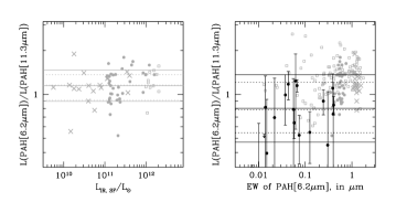
Figure 11.— Left: PAH[6.2µm]/PAH[11.3µm] ratios in star-forming galaxies from our comparison samples (crosses: Brandl et al. 2006, circles: Stierwalt et al. 2014, squares: Hill & Zakamska 2014) and the median and 68% range derived from these data (solid horizontal lines) and those presented by Diamond-Stanic & Rieke (2010), shown in dotted horizontal lines. Right: PAH ratios in the comparison samples (Brandl et al. 2006; Stierwalt et al. 2014; Hill & Zakamska 2014, grey), whether or not they have any signs of an AGN, and those of type 2 quasars in our spectroscopic sample (black points with error bars). The horizontal lines denote the mean and the standard deviation for type 2 quasars (solid lines) and the same for Seyfert galaxies (dotted lines) as presented by Diamond-Stanic & Rieke (2010). PAH ratios of type 2 quasars are more in line with those in Seyferts than those in star-forming galaxies, although there is not a strong correlation between the PAH ratios and the relative contribution of the active nucleus.

In the left panel of Figure 11, we demonstrate that our measurements of the median and the standard deviation of the PAH[6.2µm]/PAH[11.3µm] ratio among star forming galaxies are in excellent agreement with those of Diamond-Stanic & Rieke (2010), whose PAH-fitting procedures are very similar to ours. For this comparison, we pre-selected objects without any optical or infrared signatures of an AGN, so that we are evaluating purely star-forming galaxies. In the right panel, we now include PAH measurements of sources with varying degree of AGN contribution, and demonstrate the dependence of the PAH ratios as a function of the EW of PAH[6.2µm], a common measure of the fractional AGN contribution to the bolometric budget (Spoon et al., 2007). Because AGN tend to produce power-law-like emission in the mid-infrared, while star-forming galaxies (which have lower dust temperatures) rarely have strong continuum at these wavelengths, the EW of PAH[6.2µm] is high in star-forming galaxies and low in AGN, with 0.3µm being the typical dividing line (Petric et al., 2011; Stierwalt et al., 2013, 2014).

We see that type 2 quasars display relatively low EW of PAH[6.2µm], in agreement with our previous conclusion that their bolometric luminosities are dominated by AGN activity. Furthermore, despite large measurement errors, we find that the PAH[6.2µm]/PAH[11.3µm] ratio is suppressed in type 2 quasars, and again we see excellent quantitative agreement between our measurements of the median ratio and its standard deviation and those of Diamond-Stanic & Rieke (2010). The relatively low PAH[6.2µm]/PAH[11.3µm] in type 2 quasars cannot be explained by extinction which would increase this ratio: due to the silicate feature centered at 9.7µm which extends over a wide wavelength range, dust opacity is higher at 11.3µm than at 6.2µm (Weingartner & Draine, 2001; Chiar & Tielens, 2006). Therefore, we confirm that the PAH ratios appear to be affected by the quasar radiation field. However, it is not clear how much of an effect quasar radiation field may have specifically on the PAH[11.3µm]-derived star formation rates. Diamond-Stanic & Rieke (2010) argue that PAH[11.3µm] feature may be less affected than PAH[6.2µm] which traces smaller easily destroyed grains, but LaMassa et al. (2012) have argued that PAH[11.3µm], too, can be suppressed by the quasar emission resulting in an underestimate of the star formation rate.

This is suggested by Petric et al. (2015) who show that the star formation rates of type 1 quasar hosts derived from far-infrared luminosities are a factor of two-three higher than those derived from PAH[11.3µm] luminosities. Thus either the far-infrared fluxes are contaminated by the quasar resulting in an overestimate by this factor, or the PAH-emitting particles are destroyed, resulting in an underestimate by this factor, or perhaps both are true to a lesser extent. In our sample of type 2 quasars, there is unfortunately limited overlap between objects with 160µm photometry and IRS spectroscopy (28 objects, most of them with upper limits in at least one of these measurements). In the few that do have both measures of star formation (Figure 12), we do not detect any noticeable offset from the locus of star-forming galaxies, suggesting that both 160µm fluxes and PAH[11.3µm] luminosities provide consistent measures of star formation rates in these objects.

Figure 12.— Following Petric et al. (2015), we directly compare infrared luminosities of star formation in type 2 quasar hosts as derived from PAH[11.3µm] and from the 160µm flux. Solid circles show type 2 quasars with both a 160µm detection and a PAH[11.3µm] detection, whereas open circles denote upper limits in one of these measures (those objects with upper limits in both PAH[11.3µm] and 160µm flux are excluded). The solid line shows the locus expected for star forming galaxies. In type 1 quasars, Petric et al. (2015) find that 160µm photometry systematically overestimates star formation rates, or PAH[11.3µm] measurements systematically underestimate them, or both. This is not borne out by the data for type 2 quasars, although the sample is too small for a conclusive investigation.

4.4. Star formation rates from [NeII] and [NeIII] lines

Low-ionization forbidden emission lines are frequently used as a star-formation diagnostic. In Figure 13 we examine the utility of [NeII]$\lambda$12.81µm and [NeIII]$\lambda$15.56µm for use as star formation diagnostics in our sample. The line ratios of neon are clearly affected by the presence of the quasar: [NeIII]/[NeII] ratios are significantly higher in our sample of type 2 quasars than in the comparison star-forming galaxies (left). Furthermore, [NeV]$\lambda$14.32µm and [NeVI]$\lambda$7.65µm are frequently strongly detected in our sources, with [NeV]/[NeII]$\sim 1$, whereas these lines are rarely seen at all in star-forming galaxies (Farrah et al., 2007).

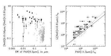
Figure 13.— Left: Neon ratios in type 2 quasars (solid black points) and in GOALS galaxies (open grey points, Inami et al. 2013), as a function of the equivalent width of the PAH[6.2µm] feature. Objects with EW of PAH[6.2µm] of $<0.3\micron$ (which includes the majority of type 2 quasars) are thought to be bolometrically dominated by the AGN. We find that these sources tend to show significantly higher [NeIII]/[NeII] ratios than those seen in pure star-forming galaxies, suggesting that AGN contributes to neon ionization. Right: Two mid-infrared star-formation diagnostics, PAH[11.3µm] luminosity and [NeII] luminosity, plotted against each other for star-forming galaxies from the GOALS sample (open grey points) and for type 2 quasars (solid black points and arrows), along with two star formation calibrations provided in the literature: the solid line is from Diamond-Stanic & Rieke (2010) and the dotted line is from Ho & Keto (2007). GOALS star forming galaxies show excellent agreement with both calibrations, but type 2 quasars show either an excess of [NeII] or a deficit of PAH[11.3µm] by about 0.35 dex, or a factor of 2.2. We choose to compare [NeII] (which is an over-estimate of star formation) with PAH[11.3µm] (which may be an underestimate of star formation) rather than 160µm fluxes (which provide upper limits on star formation) because these two values bracket actual star formation rates.

Thus [NeIII] and higher ionization lines are clearly affected by the presence of the quasar. In Figure 13, right, we explore whether [NeII] can still be safely used as a star formation diagnostic or whether it, too, has an appreciable contribution from the quasar. Using GOALS star-forming galaxies, we reproduce with high accuracy the PAH vs [NeII] calibrations from the literature (Ho & Keto, 2007; Diamond-Stanic & Rieke, 2010). The median offset between GOALS galaxies and these relationships is only $\sim 0.04$ dex, with a standard deviation around the relationships of $\sim 0.17$ dex, i.e., the quality of the PAH-[NeII] correlation is comparable to, or better, than the correlations between other star formation indicators we have discussed here.

In contrast, type 2 quasars lie systematically above the star formation relations, with a median offset of about 0.3 dex, or a factor of 2. Therefore, either the quasar contributes appreciably to the [NeII] ionization, or PAH[11.3µm] features are suppressed, or both. Because we have not found any offset between PAH-derived and 160µm-derived star formation rates (Figure 12), we suggest that the destruction of PAH[11.3µm] may not be the dominant effect and that instead the quasar dominates the photoionization of [NeII]. This finding is similar to that of Kim et al. (2006) who found that low-ionization optical emission lines, e.g., [OII]$\lambda$3727Å, may also be dominated by quasar photoionization and be poor star formation indicators.

However, the possible contribution of the quasar photoionization to the [NeII] emission does not modify our main conclusions regarding the excess of radio emission over that predicted due to star formation. Even if we were to use [NeII] as a star formation diagnostic, we would still underpredict the amount of radio emission in type 2 quasars by 0.42 / 0.78 dex (median / mean), or a factor of 2.6 / 6.0.

5. Discussion: effects of quasar on star formation and its diagnostics

Although spectral energy distribution decomposition methods assume that an AGN component and a star-forming component are simply added together to produce the overall galaxy spectrum, the two components could affect each other in a much less linear way. For example, a powerful but compact circumnuclear starburst could be further heated by the AGN, raising the apparent dust temperature beyond those encountered in star-formation templates and leading the observer to classify the source as quasar-dominated. A dusty galaxy with modest star formation rates could host a quasar; with a fortuitous geometric distribution of dust, the quasar can be hidden from view and lead to strong far-infrared emission from dust on $\gtrsim$ kpc scales, which can be mistaken for high rates of star formation. PAH-emitting particles could be destroyed by the harsh radiation from the AGN, while low-ionization emission line regions associated with star formation can get photo-ionized by the quasar, suppressing these star-formation diagnostics.

We find clear evidence for some of these effects: quasars likely suppress some PAH emission, enhance the low-ionization emission-line diagnostics, and contribute to the far-infrared emission, thereby likely affecting all mid- and far-infrared diagnostics of star formation. To minimize these effects, we choose the longest wavelength observations available to us (160µm) which have the smallest fractional contamination by the AGN, PAH[11.3µm] which is less affected by the AGN than PAH[6.2µm] and less contaminated by high-ionization line emission than PAH[7.7µm], and [NeII]$\lambda$12.81µm. These star formation measures agree with one another to within a factor of two even in quasar hosts (with [NeII] likely the most strongly affected by the quasar), giving some credence to our measured rates of star formation. Therefore, we find it highly unlikely that we have underestimated star formation rates in quasar hosts by a factor of 10, the value required to bring the observed radio fluxes in agreement with those expected from star formation alone.

The impact of quasars on the evolution of their host galaxies has emerged as a key question in modern galaxy formation models. Active black holes are now suspected in limiting galaxy masses via quasar feedback (Tabor & Binney, 1993; Silk & Rees, 1998; Springel et al., 2005), and determining the progression of star formation activity during and after an episode of black hole activity remains an interesting and unsolved problem in observational astronomy. Some studies suggest that long-term average AGN luminosity and star formation are strongly correlated, potentially due to a common supply of cold gas (Rafferty et al., 2011; Mullaney et al., 2012; Chen et al., 2013). In individual AGN, the correlations between AGN luminosity and their hosts’ star formation rates are quite weak (Shao et al., 2010; Rosario et al., 2012; Harrison et al., 2012; Stanley et al., 2015), which can largely be explained by short-term fluctuations in AGN luminosity (Hickox et al., 2014). Intriguingly, some studies have reported an apparent suppression of star formation in quasar hosts (Page et al., 2012; Barger et al., 2015), although in some cases this can be attributed to limited survey volumes and sample sizes (Harrison et al., 2012). In any case, a potential detection of a suppression in star formation for quasar hosts must be distinguished from over-ionization or destruction of the star-formation diagnostics by the quasar. This is necessary in order to be able to measure the impact of the quasar on its host galaxy.

Quasars with luminosities $\gtrsim 10^{46}$ erg s^-1 are luminous enough to easily ionize the gas over galaxy-wide scales (Liu et al., 2009; Greene et al., 2011; Hainline et al., 2013, 2014), and quasar-driven outflows (Liu et al., 2013a, b) can lead to galaxy-wide shocks (Rich et al., 2011; Hill & Zakamska, 2014; Zakamska & Greene, 2014). While circumnuclear obscuration could shield parts of the galaxy from direct quasar emission, outflows and shocks might find ways around this obstacle (Wagner et al., 2013). Physical removal of the interstellar medium suppresses subsequent star formation activity, but it would also be interesting to detect the effect of the quasar on on-going star formation in the regions affected by quasar radiation and / or quasar-driven winds. One possibility is that star formation proceeds as usual, but emission line diagnostics of star formation are strongly affected by quasar photoionization or shock excitation. This could be the origin of the decreasing [OII]$\lambda$3728Å/[OIII]$\lambda$5007Å ratio both as a function of quasar luminosity (Ho, 2005; Kim et al., 2006) and narrow-line kinematics (Zakamska & Greene, 2014). If this hypothesis is correct, then one can hide significant amounts of star formation by exposing these regions to the quasar radiation field which would bias star formation diagnostics. Another possibility is that quasar radiation and / or quasar-driven outflows are in fact suppressing on-going star formation. Developing star formation diagnostics that can distinguish between these scenarios in hosts of luminous AGN remains an interesting challenge.

6. Conclusions

The correlation between radio luminosity and narrow line gas kinematics in radio-quiet quasar host galaxies (Mullaney et al., 2013; Zakamska & Greene, 2014) suggests that there may be a physical connection between the two. This correlation has renewed the debate over the origin of the radio emission in radio-quiet quasars. One hypothesis, proposed by Condon et al. (2013) and others, cites star formation in the host galaxy as the driving mechanism behind the observed radio emission from radio quiet quasars. The median radio luminosity of radio-quiet obscured quasars is $\nu L_{\nu}$[1.4 GHz]$=1\times 10^{40}$ erg s^-1 (Zakamska & Greene, 2014), which would require 300 $M_{\odot}$ yr^-1 worth of star formation (Bell, 2003). While this is not impossible, it seems fairly high, so in this paper we ask whether the actual amount of star formation in the host galaxies is sufficient to produce the observed radio emission.

We use archival samples of star-forming galaxies to revisit calibrations of different star formation indicators: radio emission (eq. 2), single-band infrared fluxes (eq. 3-4), and PAH[11.3µm] luminosities (eq. 5-6). As long as uniform measurement methods are used – which is particularly important for PAH emission – we find excellent agreement between published calibrations and archival data, with a spread in different correlations of $\sim 0.2$ dex. With these star-formation calibrations in hand, we measure star formation rates in the hosts of quasars of different types at $z<1$ using photometric and spectroscopic data from the Spitzer and Herschel telescopes.

Using infrared colors of type 2 quasars, we demonstrate that the bolometric luminosities of the objects in our samples – estimated to range from $10^{45}$ to $10^{47}$ erg s^-1, Figure 2 – are dominated ($>50$%) by quasar emission; however, even in objects with 80% quasar contribution to the bolometric budget, more than half of the 160µm emission is due to star formation because the spectral energy distribution of starlight-heated dust peaks at much longer wavelengths than the quasar-heated dust which is concentrated on much smaller spatial scales. Thus we conclude that while our 160µm measurements strictly speaking yield upper limits on star formation, the measured rates are close to the actual values. This is confirmed by spectral energy distribution modeling of a subsample of type 2 quasars drawn from the upper decade of our luminosity distribution (Wylezalek et al., 2015).

Using 160µm fluxes in $\sim 245$ obscured and unobscured quasars, we find a broad distribution of star formation rates in quasar hosts, from median values of 6$M_{\odot}$ yr^-1 (in hosts of blue type 1 quasars) to 18$M_{\odot}$ yr^-1 (in type 2 hosts). The difference in star formation rates in hosts of type 1 and type 2 quasars has been seen in other observations (Kim et al., 2006; Zakamska et al., 2008; Hiner et al., 2009; Chen et al., 2015) and remains a challenge to the standard geometric unification model. Although statistics of molecular gas observations are still limited, existing data suggest similar availability of cold gas in hosts of type 1 and type 2 quasars (Krips et al., 2012; Villar-Martín et al., 2013), and the relatively low star formation rates of type 1 quasar hosts is in tension with the availability of cold gas in them, suggesting low star formation efficiency (Ho, 2005).

We then use mid-infrared spectra of $\sim 160$ quasars of different types to estimate the star formation rates of their hosts using spectroscopic diagnostics, especially PAH emission. We find a broad distribution of star formation rates, with a median of $\lesssim 30$ $M_{\odot}$ yr^-1. We find that PAH ratios in quasars differ from those in star forming galaxies, in excellent quantitative agreement with the findings of Diamond-Stanic & Rieke (2010), and we use PAH[11.3µm] as our primary spectroscopic star formation indicator. Further evaluating [NeII]$\lambda$12.8µm and [NeIII]$\lambda$14.3µm lines as star formation indicator, we find both to be strongly affected and likely dominated by quasar photo-ionization.

Regardless of the method used to estimate star formation in quasar hosts, we find that even the most generously computed star formation rates are insufficient to explain the observed radio emission, by about an order of magnitude. Depending on the measurement method, we measure the ratio of observed radio luminosity to that predicted due to star formation alone $L_{\rm radio,obs}/L_{\rm radio,SF}$ of 0.6$-$1.3 dex. Thus radio emission in radio-quiet quasars is unlikely to be dominated by star formation in quasar hosts and is likely associated with the quasars. Our results are in agreement with other evaluations of the star formation contribution to the radio emission of radio quiet quasars (Lal & Ho, 2010; Harrison et al., 2014).

Rosario et al. (2013) find that in AGN with $\nu L_{\nu}$[12µm]$<10^{44}$ erg s^-1 both the radio emission and the 12µm emission appear to closely follow the star-formation locus and they conclude that both 12µm and radio emission are associated with star formation (see also Bonzini et al. 2015; Padovani et al. 2015). In Figure 14 we show the discrepancy between the observed and the predicted radio emission as a function of the infrared luminosity. There is a slight trend of an increasing discrepancy toward higher 12µm luminosity. Thus it is possible that for low-luminosity AGN ($\nu L_{\nu}$[12µm]$\ll 10^{44}$ erg s^-1) the radio emission is a good measure of star formation rates in the host galaxy as Rosario et al. (2013) suggest, though some contribution to both radio and 12µm emission from the AGN at $10^{43}<\nu L_{\nu}$[12µm]$<10^{44}$ erg s^-1 appears likely in light of our results.

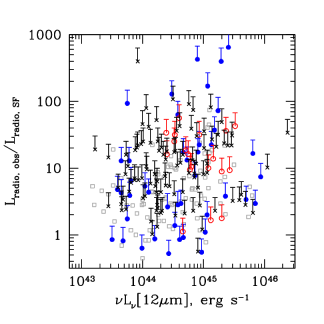
Figure 14.— The discrepancy between the observed radio emission and that expected from star formation as a function of the 12µm luminosity. Grey points are for radio non-detections, black points for radio-detected type 2 quasars, blue for PG type 1s and red for 2MASS type 1s. The discrepancy between the predicted and the observed radio emission increases with infrared luminosity (Spearman rank probability of the null hypothesis of no correlation is P[NH]$=10^{-3}$).

Regardless of the mechanism responsible for producing radio emission in the radio-quiet majority of quasars, this emission would be in addition to the radio emission produced by the host galaxy. This is well supported by Figures 4, 10 and 14, which show that rarely does the observed radio emission fall below the levels predicted to be due to star formation (and when it does, not by much). The objects whose $L_{\rm radio,obs}$ are closest to the $L_{\rm radio,SF}$ are those where the radio emission associated with the quasar is weaker than that due to star formation in the host galaxy (there are several such examples in this study and in Del Moro et al. 2013). Figure 14 suggests that as the quasar luminosity increases, there are fewer such ‘radio-silent’ objects.

There are clear cases where quasar emission dominates all bands, including far-infrared (Hony et al., 2011), and more ambiguous objects in which the lowest temperature of the dust (as measured from the spectral energy distribution) is higher than typical values seen in star-forming galaxies (Sun et al., 2014; Tsai et al., 2015) which could also be the case of a quasar dominating far-infrared emission. As we demonstrate in this paper, the radio emission in quasars is not a good estimate of star formation. Thus both $8-1000$µm fluxes and radio emission – used together or separately – may strongly overestimate star formation rates of quasar hosts (Barthel, 2006; Beelen et al., 2006), and additional cross-checks or full spectral energy distribution decomposition are required (Wang et al., 2008). Calculating star formation rates in quasar hosts is further complicated by a possibly reduced star formation efficiency which would bias diagnostics based on cold gas detection (Ho, 2005) and, for the unobscured star formation, by the strong contribution of direct or scattered light to the observed ultra-violet emission (Zakamska et al., 2005; Obied et al., 2015).

While this work rules our star formation as the origin of most radio emission from quasars, we cannot distinguish between radio emission due to compact weak jets and radio emission due to wide-angle winds. Radiatively-driven winds can produce sufficient amount of radio emission only in quasars with $L_{\rm bol}\gtrsim 3\times 10^{45}$ erg s^-1, which appears to be the threshold luminosity for driving galaxy-wide winds (Veilleux et al., 2013; Zakamska & Greene, 2014). Precise measurement of the radio luminosity function of these objects at faint radio luminosities is difficult because they are rare, so fairly high-redshift sources need to be observed with high sensitivity. Recent such work indicating a break in the radio luminosity function of quasars at fixed optical luminosity (Kimball et al., 2011; Condon et al., 2013) suggests that different mechanisms are likely responsible for the emission of radio-quiet and radio-loud sources.

This observation, and the radio vs gas kinematics correlation (Mullaney et al., 2013; Zakamska & Greene, 2014), lead us to favor radiatively-driven winds as the ultimate origin of the radio emission (Stocke et al., 1992; Wang, 2008; Jiang et al., 2010; Faucher-Giguère & Quataert, 2012; Zubovas & King, 2012; Zakamska & Greene, 2014). In this scenario, relativistic particles are accelerated on the shocks driven into the interstellar medium by the expanding wind. It may be testable by multi-wavelength observations (Nims et al., 2015), radio spectral measurements (Blundell & Kuncic, 2007) and high-resolution radio imaging. The problem of distinguishing radio emission from compact jets from radio emission as a bi-product of radiatively driven has proven especially difficult because the two mechanisms are similar in terms of energetics (Zakamska & Greene, 2014) and because a radiatively driven wind can inflate bubbles which mimic double-lobed radio morphologies, making morphology an unreliable jet / wind diagnostic (Harrison et al., 2015).

We have demonstrated that quasars and star-forming galaxies lie on different far-infrared / radio correlations: quasars show an order of magnitude more radio emission than do star-forming galaxies with the same 160µm luminosities. However, multiple groups have demonstrated that quasars, star-forming galaxies and composite sources may lie on the same total (8-1000µm) infrared / radio correlations (Crawford et al., 1996), though possibly the spread (Morić et al., 2010) or the normalization (Ivison et al., 2010) of the correlation may change slightly in the quasar-dominated regime. If radio emission of radio-quiet quasars is dominated by jets, then the infrared/radio correlation can only be explained by a strong coupling between accretion processes and jet production (Falcke et al., 1995), but finding jets on the same infrared / radio correlation as star-forming galaxies is quite surprising. If radio emission of radio-quiet quasars is dominated by radiatively driven winds, then in both quasars and star-forming galaxies the radio emission is produced by relativistic particles accelerated on shocks. What is surprising in this case is to find quasars and star-forming galaxies to be converting the same fraction of their bolometric power into shocks via completely different mechanisms (Nims et al., 2015).

Table 1160µm photometry and photometric constraints on star formation

ID	subsample	$z$	$L$[12µm]	$F_{\nu}$[160µm]	SFR	$L_{\rm radio,SF}$	$L_{\rm radio,obs}$	comment
SDSS J004340.12-005150.2	T2	0.5849	45.04	-360.3	567	40.34	-40.23	Spitzer, calibration
SDSS J005009.81-003900.6	T2	0.7276	46.05	112.7	300	40.03	41.04	Spitzer, ULIRG
SDSS J005621.72+003235.8	T2	0.4840	45.24	-72.9	95	39.47	40.97	Spitzer, type 2 quasar (PI Strauss)
SDSS J010523.62+011321.4	T2	0.2049	43.89	-230.8	55	39.20	-39.20	Spitzer, calibration
SDSS J012341.47+004435.9	T2	0.3990	44.80	-75.8	69	39.32	40.91	Spitzer, type 2 quasar (PI Strauss)

Note. — Table presented in full in the electronic edition; a small portion given here for guidance regarding format and content.

‘Subsample’ describes whether the object belongs to the type 2 sample (T2) or red type 1 sample (T1red). Herschel data for blue type 1 quasars are published by Petric et al. (2015), and Herschel data for type 2 quasars will be available in Petric et al. (in prep.) $L$[12µm] is given in units of $\log$($\nu L_{\nu}$[12µm], erg s^-1) and is set to -100 for objects undetected in both WISE-12µm and WISE-22µm.

$F_{\nu}$[160µm] measured in mJy are positive for detections (we use 25% as an estimate of the absolute uncertainty) and negative for 5$\sigma$ upper limits.

SFR gives the upper limit on the star formation rate in $M_{\odot}$ yr^-1 calculated in Section 3.2.

$L_{\rm radio,SF}$ is the upper limit on the radio emission due to star formation, given in units of $\log$($\nu L_{\nu}$[1.4GHz], erg s^-1).

$L_{\rm radio,obs}$ is the observed radio luminosity (or in the case of negative values, 5$\sigma$ upper limits) in units of $\log$($\nu L_{\nu}$[1.4GHz], erg s^-1).

Comment column describes whether the object was in the Spitzer or in the Herschel sample, whether it was targeted for pointed observations, and if so, why, or if it was covered serendipitously in observations of other targets (with the survey name given in parentheses if applicable).

Table 2IRS spectroscopy of type 2 quasars

Note. — Table presented in full in the electronic edition; a small portion given here for guidance regarding format and content.

$S$[9.7µm] is the dimensionless strength of the silicate feature (positive for absorption, negative for emission), similar to optical depth and defined in Section 2.4; typical systematic uncertainty in this measurement is 0.2 (Zakamska, 2010).

‘SL factor’ is the multiplicative factor applied to the short-low IRS orders to bring them in agreement with the long-low orders.

$L$ of Ne and PAH emission features is given in units of $10^{42}$ erg s^-1, positive for detections, negative for 3$\sigma$ upper limits, ‘NaN’ for lacking spectral coverage.

$L_{\rm radio,obs}$ is the observed radio luminosity (or in the case of negative values, 5$\sigma$ upper limits) in units of $\log$($\nu L_{\nu}$[1.4GHz], erg s^-1).

Comment column describes why the object was targeted for IRS observations.

References

- Allamandola et al. (1989) Allamandola, L. J., Tielens, A. G. G. M., & Barker, J. R. 1989, ApJS, 71, 733
- Aniano et al. (2011) Aniano, G., Draine, B. T., Gordon, K. D., & Sandstrom, K. 2011, PASP, 123, 1218
- Armus et al. (2009) Armus, L., Mazzarella, J. M., Evans, A. S., et al. 2009, PASP, 121, 559
- Barger et al. (2015) Barger, A. J., Cowie, L. L., Owen, F. N., et al. 2015, ApJ, 801, 87
- Barthel (2006) Barthel, P. D. 2006, A&A, 458, 107
- Barvainis & Antonucci (1989) Barvainis, R., & Antonucci, R. 1989, ApJS, 70, 257
- Becker et al. (1995) Becker, R. H., White, R. L., & Helfand, D. J. 1995, ApJ, 450, 559
- Beelen et al. (2006) Beelen, A., Cox, P., Benford, D. J., et al. 2006, ApJ, 642, 694
- Bell (2003) Bell, E. F. 2003, ApJ, 586, 794
- Blundell & Kuncic (2007) Blundell, K. M., & Kuncic, Z. 2007, ApJ, 668, L103
- Bohren & Huffman (1983) Bohren, C. F., & Huffman, D. R. 1983, Absorption and scattering of light by small particles (New York: Wiley)
- Bonchi et al. (2013) Bonchi, A., La Franca, F., Melini, G., Bongiorno, A., & Fiore, F. 2013, MNRAS, 429, 1970
- Bonzini et al. (2015) Bonzini, M., Mainieri, V., Padovani, P., et al. 2015, MNRAS, 453, 1079
- Brandl et al. (2006) Brandl, B. R., Bernard-Salas, J., Spoon, H. W. W., et al. 2006, ApJ, 653, 1129
- Burgarella et al. (2013) Burgarella, D., Buat, V., Gruppioni, C., et al. 2013, A&A, 554, A70
- Canalizo & Stockton (2013) Canalizo, G., & Stockton, A. 2013, ApJ, 772, 132
- Chen et al. (2013) Chen, C.-T. J., Hickox, R. C., Alberts, S., et al. 2013, ApJ, 773, 3
- Chen et al. (2015) —. 2015, ApJ, 802, 50
- Chiar & Tielens (2006) Chiar, J. E., & Tielens, A. G. G. M. 2006, ApJ, 637, 774
- Condon et al. (1998) Condon, J. J., Cotton, W. D., Greisen, E. W., et al. 1998, AJ, 115, 1693
- Condon et al. (2013) Condon, J. J., Kellermann, K. I., Kimball, A. E., Ivezić, Ž., & Perley, R. A. 2013, ApJ, 768, 37
- Crawford et al. (1996) Crawford, T., Marr, J., Partridge, B., & Strauss, M. A. 1996, ApJ, 460, 225
- Cutri et al. (2001) Cutri, R. M., Nelson, B. O., Kirkpatrick, J. D., Huchra, J. P., & Smith, P. S. 2001, in Astronomical Society of the Pacific Conference Series, Vol. 232, The New Era of Wide Field Astronomy, ed. R. Clowes, A. Adamson, & G. Bromage, 78
- Dale & Helou (2002) Dale, D. A., & Helou, G. 2002, ApJ, 576, 159
- de Grijp et al. (1987) de Grijp, M. H. K., Lub, J., & Miley, G. K. 1987, A&AS, 70, 95
- Del Moro et al. (2013) Del Moro, A., Alexander, D. M., Mullaney, J. R., et al. 2013, A&A, 549, A59
- Diamond-Stanic & Rieke (2010) Diamond-Stanic, A. M., & Rieke, G. H. 2010, ApJ, 724, 140
- Dicken et al. (2012) Dicken, D., Tadhunter, C., Axon, D., et al. 2012, ApJ, 745, 172
- Dicken et al. (2014) Dicken, D., Tadhunter, C., Morganti, R., et al. 2014, ApJ, 788, 98
- Dopita et al. (2005) Dopita, M. A., Groves, B. A., Fischera, J., et al. 2005, ApJ, 619, 755
- Falcke et al. (1995) Falcke, H., Malkan, M. A., & Biermann, P. L. 1995, A&A, 298, 375
- Farrah et al. (2007) Farrah, D., Bernard-Salas, J., Spoon, H. W. W., et al. 2007, ApJ, 667, 149
- Faucher-Giguère & Quataert (2012) Faucher-Giguère, C.-A., & Quataert, E. 2012, MNRAS, 425, 605
- Feltre et al. (2013) Feltre, A., Hatziminaoglou, E., Hernán-Caballero, A., et al. 2013, MNRAS, 434, 2426
- Fitzpatrick & Massa (1986) Fitzpatrick, E. L., & Massa, D. 1986, ApJ, 307, 286
- Frayer et al. (2006) Frayer, D. T., Fadda, D., Yan, L., et al. 2006, AJ, 131, 250
- Genzel et al. (1998) Genzel, R., Lutz, D., Sturm, E., et al. 1998, ApJ, 498, 579
- Glikman et al. (2012) Glikman, E., Urrutia, T., Lacy, M., et al. 2012, ApJ, 757, 51
- Green et al. (1986) Green, R. F., Schmidt, M., & Liebert, J. 1986, ApJS, 61, 305
- Greene et al. (2011) Greene, J. E., Zakamska, N. L., Ho, L. C., & Barth, A. J. 2011, ApJ, 732, 9
- Haas et al. (2000) Haas, M., Müller, S. A. H., Chini, R., et al. 2000, A&A, 354, 453
- Hainline et al. (2013) Hainline, K. N., Hickox, R., Greene, J. E., Myers, A. D., & Zakamska, N. L. 2013, ApJ, 774, 145
- Hainline et al. (2014) Hainline, K. N., Hickox, R. C., Greene, J. E., et al. 2014, ApJ, 787, 65
- Harrison et al. (2014) Harrison, C. M., Alexander, D. M., Mullaney, J. R., & Swinbank, A. M. 2014, MNRAS, 441, 3306
- Harrison et al. (2015) Harrison, C. M., Thomson, A. P., Alexander, D. M., et al. 2015, ApJ, 800, 45
- Harrison et al. (2012) Harrison, C. M., Alexander, D. M., Mullaney, J. R., et al. 2012, ApJ, 760, L15
- Hatziminaoglou et al. (2010) Hatziminaoglou, E., Omont, A., Stevens, J. A., et al. 2010, A&A, 518, L33
- Hayward et al. (2014) Hayward, C. C., Lanz, L., Ashby, M. L. N., et al. 2014, MNRAS, 445, 1598
- Helou et al. (1985) Helou, G., Soifer, B. T., & Rowan-Robinson, M. 1985, ApJ, 298, L7
- Hernán-Caballero & Hatziminaoglou (2011) Hernán-Caballero, A., & Hatziminaoglou, E. 2011, MNRAS, 414, 500
- Hernán-Caballero et al. (2009) Hernán-Caballero, A., Pérez-Fournon, I., Hatziminaoglou, E., et al. 2009, MNRAS, 395, 1695
- Hickox et al. (2014) Hickox, R. C., Mullaney, J. R., Alexander, D. M., et al. 2014, ApJ, 782, 9
- Hill & Zakamska (2014) Hill, M. J., & Zakamska, N. L. 2014, MNRAS, 439, 2701
- Hiner et al. (2009) Hiner, K. D., Canalizo, G., Lacy, M., et al. 2009, ApJ, 706, 508
- Ho (2005) Ho, L. C. 2005, ApJ, 629, 680
- Ho & Keto (2007) Ho, L. C., & Keto, E. 2007, ApJ, 658, 314
- Hodge et al. (2011) Hodge, J. A., Becker, R. H., White, R. L., Richards, G. T., & Zeimann, G. R. 2011, AJ, 142, 3
- Hony et al. (2011) Hony, S., Kemper, F., Woods, P. M., et al. 2011, A&A, 531, A137
- Hopkins et al. (2006) Hopkins, P. F., Hernquist, L., Cox, T. J., et al. 2006, ApJS, 163, 1
- Houck et al. (2004) Houck, J. R., Roellig, T. L., van Cleve, J., et al. 2004, ApJS, 154, 18
- Husemann et al. (2013) Husemann, B., Wisotzki, L., Sánchez, S. F., & Jahnke, K. 2013, A&A, 549, A43
- Imanishi et al. (2007) Imanishi, M., Dudley, C. C., Maiolino, R., et al. 2007, ApJS, 171, 72
- Inami et al. (2013) Inami, H., Armus, L., Charmandaris, V., et al. 2013, ApJ, 777, 156
- Ishibashi & Courvoisier (2011) Ishibashi, W., & Courvoisier, T. J.-L. 2011, A&A, 525, A118
- Ivezić et al. (2002) Ivezić, Ž., Menou, K., Knapp, G. R., et al. 2002, AJ, 124, 2364
- Ivezić et al. (2004) Ivezić, Z., Richards, G., Hall, P., et al. 2004, in Astronomical Society of the Pacific Conference Series, Vol. 311, AGN Physics with the Sloan Digital Sky Survey, ed. G. T. Richards & P. B. Hall, 347
- Ivison et al. (2010) Ivison, R. J., Magnelli, B., Ibar, E., et al. 2010, A&A, 518, L31
- Jarrett et al. (2011) Jarrett, T. H., Cohen, M., Masci, F., et al. 2011, ApJ, 735, 112
- Jiang et al. (2010) Jiang, Y.-F., Ciotti, L., Ostriker, J. P., & Spitkovsky, A. 2010, ApJ, 711, 125
- Kennicutt (1998) Kennicutt, Jr., R. C. 1998, ARA&A, 36, 189
- Kennicutt et al. (2009) Kennicutt, Jr., R. C., Hao, C.-N., Calzetti, D., et al. 2009, ApJ, 703, 1672
- Kim et al. (2006) Kim, M., Ho, L. C., & Im, M. 2006, ApJ, 642, 702
- Kimball et al. (2011) Kimball, A. E., Kellermann, K. I., Condon, J. J., Ivezić, Ž., & Perley, R. A. 2011, ApJ, 739, L29
- Kirkpatrick et al. (2012) Kirkpatrick, A., Pope, A., Alexander, D. M., et al. 2012, ApJ, 759, 139
- Kishimoto et al. (2011) Kishimoto, M., Hönig, S. F., Antonucci, R., et al. 2011, A&A, 536, A78
- Krips et al. (2012) Krips, M., Neri, R., & Cox, P. 2012, ApJ, 753, 135
- Lacy et al. (2007) Lacy, M., Sajina, A., Petric, A. O., et al. 2007, ApJ, 669, L61
- Lagos et al. (2011) Lagos, C. D. P., Padilla, N. D., Strauss, M. A., Cora, S. A., & Hao, L. 2011, MNRAS, 414, 2148
- Lal & Ho (2010) Lal, D. V., & Ho, L. C. 2010, AJ, 139, 1089
- LaMassa et al. (2012) LaMassa, S. M., Heckman, T. M., Ptak, A., et al. 2012, ApJ, 758, 1
- Laor & Behar (2008) Laor, A., & Behar, E. 2008, MNRAS, 390, 847
- Levenson et al. (2007) Levenson, N. A., Sirocky, M. M., Hao, L., et al. 2007, ApJ, 654, L45
- Liu et al. (2013a) Liu, G., Zakamska, N. L., Greene, J. E., Nesvadba, N. P. H., & Liu, X. 2013a, MNRAS, 430, 2327
- Liu et al. (2013b) —. 2013b, MNRAS, 436, 2576
- Liu et al. (2009) Liu, X., Zakamska, N. L., Greene, J. E., et al. 2009, ApJ, 702, 1098
- Magnelli et al. (2013) Magnelli, B., Popesso, P., Berta, S., et al. 2013, A&A, 553, A132
- Morić et al. (2010) Morić, I., Smolčić, V., Kimball, A., et al. 2010, ApJ, 724, 779
- Mullaney et al. (2013) Mullaney, J. R., Alexander, D. M., Fine, S., et al. 2013, MNRAS, 433, 622
- Mullaney et al. (2011) Mullaney, J. R., Alexander, D. M., Goulding, A. D., & Hickox, R. C. 2011, MNRAS, 414, 1082
- Mullaney et al. (2012) Mullaney, J. R., Daddi, E., Béthermin, M., et al. 2012, ApJ, 753, L30
- Nenkova et al. (2002) Nenkova, M., Ivezić, Ž., & Elitzur, M. 2002, ApJ, 570, L9
- Neugebauer et al. (1984) Neugebauer, G., Habing, H. J., van Duinen, R., et al. 1984, ApJ, 278, L1
- Nguyen et al. (2010) Nguyen, H. T., Schulz, B., Levenson, L., et al. 2010, A&A, 518, L5
- Nims et al. (2015) Nims, J., Quataert, E., & Faucher-Giguère, C.-A. 2015, MNRAS, 447, 3612
- Noll et al. (2009) Noll, S., Burgarella, D., Giovannoli, E., et al. 2009, A&A, 507, 1793
- Obied et al. (2015) Obied, G., Zakamska, N. L., Wylezalek, D., & Liu, G. 2015, submitted, 000, 00
- Padovani et al. (2015) Padovani, P., Bonzini, M., Kellermann, K. I., et al. 2015, MNRAS, 452, 1263
- Page et al. (2012) Page, M. J., Symeonidis, M., Vieira, J. D., et al. 2012, Nature, 485, 213
- Peeters et al. (2004) Peeters, E., Spoon, H. W. W., & Tielens, A. G. G. M. 2004, ApJ, 613, 986
- Petric et al. (2015) Petric, A. O., Ho, L. C., Flagey, N. J. M., & Scoville, N. Z. 2015, ApJS, 219, 22
- Petric et al. (2011) Petric, A. O., Armus, L., Howell, J., et al. 2011, ApJ, 730, 28
- Pier & Krolik (1992) Pier, E. A., & Krolik, J. H. 1992, ApJ, 401, 99
- Polletta et al. (2007) Polletta, M., Tajer, M., Maraschi, L., et al. 2007, ApJ, 663, 81
- Rafferty et al. (2011) Rafferty, D. A., Brandt, W. N., Alexander, D. M., et al. 2011, ApJ, 742, 3
- Reyes et al. (2008) Reyes, R., Zakamska, N. L., Strauss, M. A., et al. 2008, AJ, 136, 2373
- Rich et al. (2011) Rich, J. A., Kewley, L. J., & Dopita, M. A. 2011, ApJ, 734, 87
- Richards et al. (2006) Richards, G. T., Lacy, M., Storrie-Lombardi, L. J., et al. 2006, ApJS, 166, 470
- Rieke et al. (2004) Rieke, G. H., Young, E. T., Engelbracht, C. W., et al. 2004, ApJS, 154, 25
- Rosario et al. (2013) Rosario, D. J., Burtscher, L., Davies, R., et al. 2013, ApJ, 778, 94
- Rosario et al. (2012) Rosario, D. J., Santini, P., Lutz, D., et al. 2012, A&A, 545, A45
- Roussel et al. (2001) Roussel, H., Sauvage, M., Vigroux, L., & Bosma, A. 2001, A&A, 372, 427
- Sánchez-Portal et al. (2014) Sánchez-Portal, M., Marston, A., Altieri, B., et al. 2014, Experimental Astronomy, 37, 453
- Sanders et al. (1988) Sanders, D. B., Soifer, B. T., Elias, J. H., et al. 1988, ApJ, 325, 74
- Savage & Oliver (2007) Savage, R. S., & Oliver, S. 2007, ApJ, 661, 1339
- Schmidt & Green (1983) Schmidt, M., & Green, R. F. 1983, ApJ, 269, 352
- Shang et al. (2011) Shang, Z., Brotherton, M. S., Wills, B. J., et al. 2011, ApJS, 196, 2
- Shao et al. (2010) Shao, L., Lutz, D., Nordon, R., et al. 2010, A&A, 518, L26
- Shen et al. (2011) Shen, Y., Richards, G. T., Strauss, M. A., et al. 2011, ApJS, 194, 45
- Shi et al. (2007) Shi, Y., Ogle, P., Rieke, G. H., et al. 2007, ApJ, 669, 841
- Silk & Rees (1998) Silk, J., & Rees, M. J. 1998, A&A, 331, L1
- Smith et al. (2007) Smith, J. D. T., Draine, B. T., Dale, D. A., et al. 2007, ApJ, 656, 770
- Smith et al. (2002) Smith, P. S., Schmidt, G. D., Hines, D. C., Cutri, R. M., & Nelson, B. O. 2002, ApJ, 569, 23
- Spoon & Holt (2009) Spoon, H. W. W., & Holt, J. 2009, ApJ, 702, L42
- Spoon et al. (2007) Spoon, H. W. W., Marshall, J. A., Houck, J. R., et al. 2007, ApJ, 654, L49
- Springel et al. (2005) Springel, V., Di Matteo, T., & Hernquist, L. 2005, MNRAS, 361, 776
- Stanley et al. (2015) Stanley, F., Harrison, C. M., Alexander, D. M., et al. 2015, MNRAS, 453, 591
- Stierwalt et al. (2013) Stierwalt, S., Armus, L., Surace, J. A., et al. 2013, ApJS, 206, 1
- Stierwalt et al. (2014) Stierwalt, S., Armus, L., Charmandaris, V., et al. 2014, ApJ, 790, 124
- Stocke et al. (1992) Stocke, J. T., Morris, S. L., Weymann, R. J., & Foltz, C. B. 1992, ApJ, 396, 487
- Sturm et al. (2006) Sturm, E., Hasinger, G., Lehmann, I., et al. 2006, ApJ, 642, 81
- Sun et al. (2014) Sun, A.-L., Greene, J. E., Zakamska, N. L., & Nesvadba, N. P. H. 2014, ApJ, 790, 160
- Symeonidis et al. (2008) Symeonidis, M., Willner, S. P., Rigopoulou, D., et al. 2008, MNRAS, 385, 1015
- Tabor & Binney (1993) Tabor, G., & Binney, J. 1993, MNRAS, 263, 323
- Tsai et al. (2015) Tsai, C.-W., Eisenhardt, P. R. M., Wu, J., et al. 2015, ApJ, 805, 90
- U et al. (2012) U, V., Sanders, D. B., Mazzarella, J. M., et al. 2012, ApJS, 203, 9
- Urry & Padovani (1995) Urry, C. M., & Padovani, P. 1995, PASP, 107, 803
- Veilleux (1991) Veilleux, S. 1991, ApJ, 369, 331
- Veilleux et al. (2013) Veilleux, S., Meléndez, M., Sturm, E., et al. 2013, ApJ, 776, 27
- Villar-Martín et al. (2013) Villar-Martín, M., Rodríguez, M., Drouart, G., et al. 2013, MNRAS, 434, 978
- Wagner et al. (2013) Wagner, A. Y., Umemura, M., & Bicknell, G. V. 2013, ApJ, 763, L18
- Wang (2008) Wang, J.-M. 2008, ApJ, 682, L81
- Wang et al. (2008) Wang, R., Carilli, C. L., Wagg, J., et al. 2008, ApJ, 687, 848
- Weingartner & Draine (2001) Weingartner, J. C., & Draine, B. T. 2001, ApJ, 548, 296
- White et al. (1997) White, R. L., Becker, R. H., Helfand, D. J., & Gregg, M. D. 1997, ApJ, 475, 479
- White et al. (2007) White, R. L., Helfand, D. J., Becker, R. H., Glikman, E., & de Vries, W. 2007, ApJ, 654, 99
- Wright et al. (2010) Wright, E. L., Eisenhardt, P. R. M., Mainzer, A. K., et al. 2010, AJ, 140, 1868
- Wylezalek et al. (2015) Wylezalek, D., Zakamska, N., Liu, G., & Obied, G. 2015, submitted, 000, 00
- Zakamska (2010) Zakamska, N. L. 2010, Nature, 465, 60
- Zakamska et al. (2008) Zakamska, N. L., Gómez, L., Strauss, M. A., & Krolik, J. H. 2008, AJ, 136, 1607
- Zakamska & Greene (2014) Zakamska, N. L., & Greene, J. E. 2014, MNRAS, 442, 784
- Zakamska et al. (2004) Zakamska, N. L., Strauss, M. A., Heckman, T. M., Ivezić, Ž., & Krolik, J. H. 2004, AJ, 128, 1002
- Zakamska et al. (2003) Zakamska, N. L., et al. 2003, AJ, 126, 2125
- Zakamska et al. (2005) —. 2005, AJ, 129, 1212
- Zakamska et al. (2006) —. 2006, AJ, 132, 1496
- Zubovas & King (2012) Zubovas, K., & King, A. 2012, ApJ, 745, L34