Convexity in Tree Spaces

Abstract

We study the geometry of metrics and convexity structures on the space of phylogenetic trees, which is here realized as the tropical linear space of all ultrametrics. The ${\rm CAT}(0)$-metric of Billera-Holmes-Vogtman arises from the theory of orthant spaces. While its geodesics can be computed by the Owen-Provan algorithm, geodesic triangles are complicated. We show that the dimension of such a triangle can be arbitrarily high. Tropical convexity and the tropical metric behave better. They exhibit properties desirable for geometric statistics, such as geodesics of small depth.

05C05, 30F45, 52B40, 68U05, 92D15

1 Introduction

A finite metric space with $m$ elements is represented by a nonnegative symmetric $m\times m$-matrix $D=(d_{ij})$ with zero entries on the diagonal such that all triangle inequalities are satisfied:

$$d_{ik}\leq d_{ij}+d_{jk}\quad\hbox{for all}\,\,\,i,j,k\,\,\,\hbox{in}\,\,\,[m]:=\{1,2,\ldots,m\}.$$

The set of all such metrics is a full-dimensional closed polyhedral cone, known as the metric cone, in the space $\mathbb{R}^{\binom{m}{2}}$ of symmetric matrices with vanishing diagonal. For many applications one requires the following strengthening of the triangle inequalities:

(1) $$\quad d_{ik}\leq{\rm max}(d_{ij},d_{jk})\quad\hbox{for all}\,\,\,i,j,k\in[m].$$

If (1) holds then the metric space $D$ is called an ultrametric. The set of all ultrametrics contains the ray $\mathbb{R}_{\geq 0}{\bf 1}$ spanned by the all-one metric ${\bf 1}$, which is defined by $d_{ij}=1$ for $1\leq i<j\leq m$. The image of the set of ultrametrics in the quotient space $\mathbb{R}^{\binom{m}{2}}\!/\mathbb{R}{\bf 1}$ is denoted $\mathcal{U}_{m}$ and called the space of ultrametrics. It is known in tropical geometry [5, 19] and in phylogenetics [14, 26] that $\mathcal{U}_{m}$ is the support of a pointed simplicial fan of dimension $m-2$. That fan has $2^{m}{-}m{-}2$ rays, namely the clade metrics $D_{\sigma}$. A clade $\sigma$ is a proper subset of $[m]$ with at least two elements, and $D_{\sigma}$ is the ultrametric whose $ij$-th entry is $0$ if $i,j\in\sigma$ and $1$ otherwise. Each cone in that fan structure consists of all ultrametrics whose tree has a fixed topology. We encode each topology by a nested set [11], i.e. a set of clades $\{\sigma_{1},\sigma_{2},\ldots,\sigma_{d}\}$ such that

(2) $$\sigma_{i}\subset\sigma_{j}\quad\hbox{or}\quad\sigma_{j}\subset\sigma_{i}\quad\hbox{or}\quad\sigma_{i}\,\cap\,\sigma_{j}=\emptyset\qquad\hbox{for all}\,\,\,1\leq i<j\leq d.$$

Here $d$ can be any integer between $1$ and $m-2$. The nested set represents the $d$-dimensional cone spanned by $\{D_{\sigma_{1}},D_{\sigma_{2}},\ldots,D_{\sigma_{d}}\}\,$ inside $\,\mathcal{U}_{m}\subset\mathbb{R}^{\binom{m}{2}}\!/\mathbb{R}{\bf 1}$. For an illustration of this fan structure, consider equidistant trees on $m=4$ taxa. The space of these is a two-dimensional fan over the Petersen graph, shown on the left in Fig. 1.

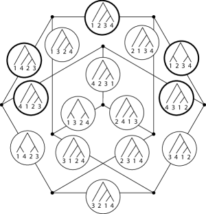
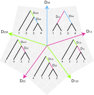
Figure 1: The space of ultrametrics $\mathcal{U}_{4}$ is a two-dimensional fan with $15$ maximal cones. Their adjacency forms a Petersen graph. Depicted on the right is a cycle of five cones.

At this point it is essential to stress that we have not yet defined convexity or a metric on $\mathcal{U}_{m}$. So far, our tree space $\mathcal{U}_{m}$ is nothing but a subset of $\mathbb{R}^{\binom{m}{2}}\!/\mathbb{R}{\bf 1}$. It is the support of the fan described above, but even that fan structure is not unique. There are other meaningful fan structures, classified by the building sets in [11]. An important one is the $\tau$-space of [14, §2], known to combinatorialists as the order complex of the partition lattice [5].

The aim of this paper is to compare different geometric structures on $\mathcal{U}_{m}$, and to explore statistical issues. The first geometric structure is the metric proposed by Billera, Holmes and Vogtman in [7]. In their setting, each cone is right-angled. The BHV metric is the unique metric on $\mathcal{U}_{m}$ that restricts to the usual Euclidean distance on each such right-angled cone. For this to be well-defined, we must fix a simplicial fan structure on $\mathcal{U}_{m}$. This issue is subtle, as explained by Gavruskin and Drummond in [14]. The BHV metric has the ${\rm CAT}(0)$-property [7, §4.2]. This implies that between any two points there is a unique geodesic.

Owen and Provan [23] proved that these geodesics can be computed in polynomial time. In Section 2, we present a detailed review and analysis. This is done in the setting of orthant spaces $\mathcal{F}_{\Omega}$ associated with flag simplicial complexes $\Omega$.

In Section 3 we study geodesically closed subsets of an orthant space $\mathcal{F}_{\Omega}$, with primary focus on geodesic triangles. Problem 3.3 asks whether these are always closed. Our main result, Theorem 3.10, states that the dimension of a geodesic triangle can be arbitrarily large. The same is concluded for the tree space $\mathcal{U}_{m}$ in Corollary 3.12. For experts in phylogenetics, we note that our results are not restricted to equidistant trees. They extend naturally to the more familiar BHV space for all rooted trees.

Tropical geometry [19] furnishes an alternative geometric structure on $\mathcal{U}_{m}$, via the graphic matroid of the complete graph [19, Example 4.2.14]. More generally, for any matroid $M$, the tropical linear space ${\rm Trop}(M)$ is tropically convex by [19, Proposition 5.2.8], and it is a metric space with the tropical distance to be defined in (14). Tropical geodesics are not unique, but tropically convex sets have desirable properties. In particular, triangles are always $2$-dimensional.

Section 5 offers an experimental study of Euclidean geodesics and tropical segments. The latter are better than the former with regard to depth, i.e. the largest codimension of cones traversed. This is motivated by the issue of stickiness in geometric statistics [16, 20]. Section 6 advocates tropical geometry for statistical applications. Starting from Nye’s principal component analysis in [22], we propose two basic tools for future data analyses: computation of tropical centroids, and nearest-point projection onto tropical linear spaces.

In a statistical context, it can be advantageous to replace $\,\mathcal{U}_{m}$ by a compact subspace. We define compact tree space $\,\mathcal{U}_{m}^{[1]}\,$ to be the image in $\mathcal{U}_{m}$ of the set of ultrametrics $D=(d_{ij})$ that satisfy ${\rm max}_{ij}\{d_{ij}\}=1$. This is a polyhedral complex consisting of one convex polytope for each nested set $\{\sigma_{1},\sigma_{2},\ldots,\sigma_{d}\}$. In the notation of (7), this polytope consists of all $(\ell_{1},\ell_{2},\ldots,\ell_{d})\in[0,1]^{d}$ such that $\ell_{i_{1}}{+}\ell_{i_{2}}{+}\cdots{+}\ell_{i_{d}}\leq 1$ whenever $\sigma_{i_{1}}\subset\sigma_{i_{2}}\subset\cdots\subset\sigma_{i_{d}}$. In phylogenetics, these are equidistant trees of height $\frac{1}{2}$ with a fixed tree topology. For instance, $\mathcal{U}_{4}^{[1]}$ is a polyhedral surface, consisting of $12$ triangles and $3$ squares, glued along $10$ edges.

2 Orthant Spaces

In order to understand the geometry of tree spaces, we work in the more general setting of globally nonpositively curved (NPC) spaces. This was suggested by Miller, Owen and Provan in [21, §6]. We follow their set-up.

Consider a simplicial complex $\Omega$ on the ground set $[n]=\{1,2,\ldots,n\}$. We say that $\Omega$ is a flag complex if all its minimal non-faces have two elements. Equivalently, a flag complex is determined by its edges: a subset $\sigma$ of $[n]$ is in $\Omega$ if and only if $\{i,j\}\in\Omega$ for all $i,j\in\sigma$. Every simplicial complex $\Omega$ on $[n]$ determines a simplicial fan $\mathcal{F}_{\Omega}$ in $\mathbb{R}^{n}$. The cones in $\mathcal{F}_{\Omega}$ are the orthants $\mathcal{O}_{\sigma}={\rm pos}\{e_{i}:i\in\sigma\}$ where $\sigma\in\Omega$. Here $\{e_{1},e_{2},\ldots,e_{n}\}$ is the standard basis of $\mathbb{R}^{n}$. We say that $\mathcal{F}_{\Omega}$ is an orthant space if the underlying simplicial complex $\Omega$ is flag. The support of the fan $\mathcal{F}_{\Omega}$ is turned into a metric space by fixing the usual Euclidean distance on each orthant. A path of minimal length between two points is called a geodesic.

Proposition 2.1.

Let $\mathcal{F}_{\Omega}$ be an orthant space. For any two points $v$ and $w$ in $\mathcal{F}_{\Omega}$ there exists a unique geodesic between $v$ and $w$. This geodesic is denoted $G(v,w)$.

The uniqueness of geodesics is attributed to Gromov. We refer to [4, Theorem 2.12] and [21, Lemma 6.2] for expositions and applications of this important result. The main point is that orthant spaces, with their Euclidean metric as above, satisfy the ${\rm CAT}(0)$ property, provided $\Omega$ is flag. This property states that chords in triangles are no longer than the corresponding chords in Euclidean triangles. The metric spaces $\mathcal{F}_{\Omega}$ coming from flag complexes $\Omega$ are called global NPC orthant spaces in [21]. For simplicity we here use the term orthant space for $\mathcal{F}_{\Omega}$.

Example 2.2.

Let $n=3$ and $\Omega=\{12,23,31\}$, i.e. the $3$-cycle. The fan $\mathcal{F}_{\Omega}$ is the boundary of the nonnegative orthant in $\mathbb{R}^{3}$. This is not an orthant space because $\Omega$ is not flag. Some geodesics in $\mathcal{F}_{\Omega}$ are not unique: the points $v=(1,0,0)$ and $w=(0,1,1)$ have distance $\sqrt{5}$, and there are two geodesics: one passing through $(0,\frac{1}{2},0)$ and the other passing through $(0,0,\frac{1}{2})$. By contrast, let $n=4$ and $\Omega=\{12,23,34,41\}$, i.e. the $4$-cycle. Then $\mathcal{F}_{\Omega}$ is a $2$-dimensional orthant space in $\mathbb{R}^{4}$. The Euclidean geodesics on that surface are unique.

The problem of computing the unique geodesics was solved by Owen and Provan in [23]. In [23], the focus was on tree space of Billera-Holmes-Vogtman [7]. It was argued in [21, Corollary 6.19] that the result extends to arbitrary orthant spaces. Owen and Provan gave a polynomial-time algorithm whose input consists of two points $v$ and $w$ in $\mathcal{F}_{\Omega}$ and whose output is the geodesic $G(v,w)$. We shall now describe their method.

Let $\sigma$ be a simplex in a flag complex $\Omega$, with corresponding orthant $\mathcal{O}_{\sigma}$ in $\mathcal{F}_{\Omega}$. Consider a point $v=\sum_{i\in\sigma}v_{i}e_{i}$ in $\mathcal{O}_{\sigma}$ and any face $\tau$ of $\sigma$. We write $v_{\tau}=\sum_{i\in\tau}v_{i}e_{i}$ for the projection of $v$ into $\mathcal{O}_{\tau}$. Its Euclidean length $||v_{\tau}||=\bigl{(}\sum_{i\in\tau}v_{i}^{2}\bigr{)}^{1/2}$ is called the projection length.

We now assume that $\Omega$ is pure $(d-1)$-dimensional, i.e. all maximal simplices in $\Omega$ have the same dimension $d-1$. This means that all maximal orthants in $\mathcal{F}_{\Omega}$ have dimension $d$. Consider two general points $v$ and $w$ in the interiors of full-dimensional orthants $\mathcal{O}_{\sigma}$ and $\mathcal{O}_{\tau}$ of $\mathcal{F}_{\Omega}$ respectively. We also assume that $\sigma\cap\tau=\emptyset$. Combinatorially, the geodesic $G(v,w)$ is then encoded by a pair $({\cal A},{\cal B})$ where ${\cal A}=(A_{1},\ldots,A_{q})$ is an ordered partition of $\sigma=\{\sigma_{1},\ldots,\sigma_{d}\}$ and ${\cal B}=(B_{1},\ldots,B_{q})$ is an ordered partition of $\tau=\{\tau_{1},\ldots,\tau_{d}\}$. These two partitions have the same number $q$ of parts, and they satisfy the following three properties:

• (P1) for all pairs $i>j$, the set $A_{i}\cup B_{j}$ is a simplex in $\Omega$.

• (P2) $||v_{A_{1}}||/||w_{B_{1}}||\,\leq\,||v_{A_{2}}||/||w_{B_{2}}||\,\leq\,\cdots\,\leq\,||v_{A_{q}}||/||w_{B_{q}}||$.

• (P3) For $i=1,\ldots,q$, there do not exist nontrivial partitions $L_{1}\cup L_{2}$ of $A_{i}$ and $R_{1}\cup R_{2}$ of $B_{i}$ such that $R_{1}\cup L_{2}\in\Omega$ and $\,||v_{L_{1}}||/||w_{R_{1}}||\,<\,||v_{L_{2}}||/||w_{R_{2}}||$.

The following result is due to Owen and Provan [23]. They proved it for the case of BHV tree space. The general result is stated in [21, Corollary 6.19].

Theorem 2.3 (Owen-Provan).

Given points $v,w\in\mathcal{F}_{\Omega}$ satisfying the hypotheses above, there exists a unique ordered pair of partitions $({\cal A},{\cal B})$ satisfying (P1), (P2), (P3). The geodesic is a sequence of $q+1$ line segments, $G(v,w)=[v,u^{1}]\cup[u^{1},u^{2}]\cup\cdots\cup[u^{q},w]$. Its length equals

(3) $$d(v,w)\,=\,\sqrt{\mathop{\sum}_{j=1}^{q}{\bigl{(}\,||v_{A_{j}}||\,+\,||w_{B_{j}}||\,\bigr{)}^{2}}}.$$

In particular, $({\cal A},{\cal B})$ is the unique pair of ordered partitions that minimizes (3). The breakpoint $u^{i}$ lives in the orthant of $\mathcal{F}_{\Omega}$ that is indexed by $\bigcup_{j=1}^{i-1}B_{j}\cup\bigcup_{j=i+1}^{q}A_{j}$. Setting $u^{0}=v$, the coordinates of the breakpoints are computed recursively by the formulas

(4) $$\qquad u^{i}_{k}\,\,=\,\,\frac{||u^{i-1}_{A_{i}}||\cdot w_{k}+||w_{B_{i}}||\cdot u^{i-1}_{k}}{||u^{i-1}_{A_{i}}||+||w_{B_{i}}||}\qquad\qquad\qquad\qquad\hbox{for}\,\,\,k\in\bigcup_{j=1}^{i-1}{B_{j}},$$

(5) $$\qquad u^{i}_{l}\,=\,\frac{u^{i-1}_{l}}{||u^{i-1}_{A_{j}}||}\cdot\frac{||w_{B_{i}}||\cdot||u^{i-1}_{A_{j}}||-||u^{i-1}_{A_{i}}||\cdot||w_{B_{j}}||}{||u^{i-1}_{A_{i}}||+||w_{B_{i}}||}\quad\hbox{for}\,\,\,\,l\in A_{j},\,\,i+1\leq j\leq q.$$

Computing the geodesic between $v$ and $w$ in the orthant space $\mathcal{F}_{\Omega}$ means identifying the optimal pair $(\mathcal{A},\mathcal{B})$ among all pairs. This is a combinatorial optimization problem. Owen and Provan [23] gave a polynomial-time algorithm for solving this.

We implemented this algorithm in Maple. Our code works for any flag simplicial complex $\Omega$ and for any points $v$ and $w$ in the orthant space $\mathcal{F}_{\Omega}$, regardless of whether they satisfy the hypotheses of Theorem 2.3. The underlying geometry is as follows:

Theorem 2.4.

The degenerate cases not covered by Theorem 2.3 are dealt with as follows: (1) If $\sigma\cap\tau\neq\emptyset$, then an ordered pair of partitions $({\cal A},{\cal B})$ is constructed for $(\sigma\backslash\tau,\,\tau\backslash\sigma)$. The breakpoint $u^{i}$ lives in the orthant of $\mathcal{F}_{\Omega}$ indexed by $\bigcup_{j=1}^{i-1}{B_{j}}\cup\bigcup_{j=i+1}^{q}{A_{j}}\cup(\sigma\cap\tau)$. It satisfies

(6) $$\qquad u^{i}_{k}\,=\,\,\frac{||u^{i-1}_{A_{i}}||\cdot w_{k}+||w_{B_{i}}||\cdot u^{i-1}_{k}}{||u^{i-1}_{A_{i}}||+||w_{B_{i}}||}\qquad\hbox{for}\,\,\,k\in\sigma\cap\tau.$$

(2) If $|\sigma|<d$ or $|\tau|<d$, i.e. $v$ or $w$ is in a lower-dimensional orthant of $\mathcal{F}_{\Omega}$, then we allow one (but not both) of the parts $A_{i}$ and $B_{i}$ to be empty, and we replace (P2) by

• (P2’) $\quad||v_{A_{i}}||\cdot||w_{B_{i+1}}||\,\leq\,||w_{B_{i}}||\cdot||v_{A_{i+1}}||\quad$ for $\,\,1\leq i\leq q-1$.

We still get an ordered pair $({\cal A},{\cal B})$ satisfying (P1), (P2’), (P3), but it may not be unique. If $i\geq 0$ is the largest index with $A_{i}=\emptyset$ and $j\leq q+1$ is the smallest index with $B_{j}=\emptyset$, then $G(v,w)$ is a sequence of $j-i-1$ segments. The breakpoints are given in (4), (5), (6).
(3) Now, the length of the geodesic $G(v,w)$ is equal to

$$d(v,w)\,\,=\,\,\sqrt{\mathop{\sum}_{k\in\sigma\cap\tau}{(v_{k}-w_{k})^{2}}\,+\,\mathop{\sum}_{j=1}^{q}{(||v_{A_{j}}||+||w_{B_{j}}||)^{2}}}.$$

Proof 2.5.

This is an extension of the discussion for BHV tree space in [23, §4].

Our primary object of interest is the space of ultrametrics $\,\mathcal{U}_{m}$. We shall explain its metric structure as an orthant space. It is crucial to note that this structure is not unique. Indeed, any polyhedral fan $\Sigma$ in $\mathbb{R}^{d}$ can be refined to a simplicial fan with $n$ rays whose underlying simplicial complex $\Omega$ is flag. That fan still lives in $\mathbb{R}^{d}$, whereas the orthant space $\mathcal{F}_{\Omega}$ lives in $\mathbb{R}^{n}$. There is a canonical piecewise-linear isomorphism between $\mathcal{F}_{\Omega}$ and the support $|\Sigma|$, and the Euclidean metric on the former induces the metric on the latter. The resulting metric on $|\Sigma|$ depends on the choice of simplicial subdivision. A different $\Omega$ gives a different metric.

Example 2.6.

Let $d=2$ and $\Sigma=\mathbb{R}_{\geq 0}^{2}$ be the cone spanned by $v^{1}=(1,0)$ and $v^{2}=(0,1)$. In the usual metric on $\Sigma$, the distance between $v^{1}$ and $v^{2}$ is $\sqrt{2}$, and the geodesic passes through $(\frac{1}{2},\frac{1}{2})$. We refine $\Sigma$ by adding the ray spanned by $v^{3}=(1,1)$. The simplicial complex $\Omega$ has facets $13$ and $23$, and $\mathcal{F}_{\Omega}$ is the fan in $\mathbb{R}^{3}$ with maximal cones ${\rm pos}(e_{1},e_{3})$ and ${\rm pos}(e_{2},e_{3})$. The map from this orthant space onto $\Sigma$ induces a different metric. In that new metric, the distance between $v^{1}$ and $v^{2}$ is $2$, and the geodesic is the cone path passing through $(0,0)$.

Let $n=2^{m}-m-2$. The standard basis vectors in $\mathbb{R}^{n}$ are denoted $e_{\sigma}$, one for each clade $\sigma$ on $[m]$. Let $\Omega$ be the flag simplicial complex whose simplices are the nested sets $\{\sigma_{1},\ldots,\sigma_{d}\}$ as defined in (2). The piecewise-linear isomorphism from the orthant space $\mathcal{F}_{\Omega}$ to $\mathcal{U}_{m}$ takes the basis vector $e_{\sigma}$ to the clade metric $D_{\sigma}$, and this induces the BHV metric on $\mathcal{U}_{m}$. Each orthant in $\mathcal{F}_{\Omega}$ represents the set of all equidistant trees in $\mathcal{U}_{m}$ that have a fixed topology.

In Section 1, each ultrametric $D=(d_{ij})$ is an element of $\mathbb{R}^{\binom{m}{2}}\!/\mathbb{R}\mathbf{1}$. It has a unique representation

(7) $$D\,\,=\,\,\ell_{1}D_{\sigma_{1}}+\ell_{2}D_{\sigma_{2}}+\cdots+\ell_{d}D_{\sigma_{d}},$$

where $\{\sigma_{1},\ldots,\sigma_{d}\}\in\Omega$ and $\ell_{1},\ldots,\ell_{d}\geq 0$. The coefficient $\ell_{i}$ is twice the length of the edge labeled $\sigma_{i}$ in the tree given by $D$. It can be recovered from $D$ by the formula

(8) $$\ell_{i}\,\,=\,\,{\rm min}\bigl{\{}d_{rt}\,:\,r\in\sigma_{i},t\not\in\sigma_{i}\bigr{\}}\,\,-\,\,{\rm max}\bigl{\{}d_{rs}\,:\,r,s\in\sigma_{i}\bigr{\}}.$$

The maximal nested sets have cardinality $m-2$, so this is the dimension of the orthant space $\mathcal{F}_{\Omega}$. The number of maximal nested sets is $(2m-3)!!=1\cdot 3\cdot 5\cdot\cdots\cdot(2m-3)$. For instance, Fig. 1 shows that $\mathcal{U}_{4}$ is consists of $15$ two-dimensional cones and $10$ rays.

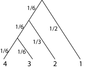
Figure 2: The equidistant tree in $\mathcal{U}_{4}^{[1]}$ discussed in Example 2.7.

Example 2.7.

The equidistant tree in Fig. 2 corresponds to the ultrametric

$$D\,=\,(d_{12},d_{13},d_{14},d_{23},d_{24},d_{34})\,=\,\bigl{(}1,1,1,\frac{2}{3},\frac{2}{3},\frac{1}{3}\bigr{)}\,\,\,\in\,\,\,\mathcal{U}_{4}^{[1]}\,\,\subset\,\,\mathcal{U}_{4}.$$

The clade metrics for the two internal edges are

$$D_{\sigma_{1}}=D_{{34}}=(1,1,1,1,1,0)\quad\hbox{and}\quad D_{\sigma_{2}}=D_{{234}}=(1,1,1,0,0,0).$$

The formula (8) gives $\ell_{1}=\ell_{2}=1/3$. Since all vectors live in $\mathbb{R}^{6}$ modulo $\mathbb{R}{\bf 1}$, we have

$$\ell_{1}D_{\sigma_{1}}+\ell_{2}D_{\sigma_{2}}\,=\,\bigl{(}\frac{2}{3},\frac{2}{3},\frac{2}{3},\frac{1}{3},\frac{1}{3},0\bigr{)}\,\,=\,\,D.$$

But, the orthant space that endows $\,\mathcal{U}_{4}$ with its metric lives in $\mathbb{R}^{10}$, and not in $\mathbb{R}^{6}/\mathbb{R}{\bf 1}$.

We close this section by reiterating this extremely important remark. In Section 1 we introduced the set $\,\mathcal{U}_{m}$ of ultrametrics as a subset of a low-dimensional ambient space, having dimension $\binom{m}{2}-1$. In Section 2 we elevated $\mathcal{U}_{m}$ to live in a high-dimensional ambient space, having dimension $2^{m}-m-2$. It is only the latter realization, as an orthant space, that is used when we compute Euclidean distances. In other words, when we compute geodesics in the BHV metric on tree space, we use the coordinates $\ell_{1},\ldots,\ell_{d}$. These are local coordinates on the right-angled cones. The coordinates $d_{12},\ldots,d_{(m-1)m}$ are never to be used for computing BHV geodesics.

3 Geodesic Triangles

Biologists are interested in BHV tree space as a statistical tool for studying evolution. The geometric structures in [7, 21] are motivated by applications such as [22]. This requires a notion of convexity.

We fix a flag simplicial complex $\Omega$ on $[n]$. The orthant space $\mathcal{F}_{\Omega}\subset\mathbb{R}^{n}$ with its intrinsic Euclidean metric has unique geodesics $G(v,w)$ as in Theorems 2.3 and 2.4. A subset $T$ of $\mathcal{F}_{\Omega}$ is called geodesically convex if, for any two points $v,w\in T$, the unique geodesic $G(v,w)$ is contained in $T$.

Given a subset $S$ of $\mathcal{F}_{\Omega}$, its geodesic convex hull ${\rm gconv}(S)$ is the smallest geodesically convex set in $\mathcal{F}_{\Omega}$ that contains $S$. If $S=\{v^{1},v^{2},\ldots,v^{s}\}$ is a finite set then we say that ${\rm gconv}(S)$ is a geodesic polytope. If $s=2$ then we recover the geodesic segment $\,{\rm gconv}(v^{1},v^{2})=G(v^{1},v^{2})$. If $s=3$ then we obtain a geodesic triangle ${\rm gconv}(S)={\rm gconv}(v^{1},v^{2},v^{3})$. The main point of this section is to demonstrate that geodesic triangles are rather complicated objects.

We begin with an iterative scheme for computing geodesic polytopes. Let $S$ be any subset of $\mathcal{F}_{\Omega}$. Then we can form the union of all geodesics with endpoints in $S$:

$$g(S)\,\,=\,\,\bigcup_{v,w\in S}{G(v,w)}.$$

For any integer $t\geq 1$, define $g^{t}(S)$ recursively as $g^{t}(S)=g(g^{t-1}(S))$, with $g^{0}(S)=S$.

Lemma 3.1.

Let $S$ be a set of points in $\mathcal{F}_{\Omega}$. Then its geodesic convex hull equals

$$gconv(S)\,\,=\,\,\bigcup_{t=0}^{\infty}{g^{t}(S)}.$$

In words, the geodesic convex hull of $S$ is the set of all points in $\mathcal{F}_{\Omega}$ that can be generated in finitely many steps from $S$ by taking geodesic segments.

Proof 3.2.

If $T$ is a subset of ${\rm gconv}(S)$ then $g(T)\subseteq{\rm gconv}(S)$. By induction on $t$, we see that $\,g^{t}(S)\subseteq{\rm gconv}(S)$ for all $t\in\mathbb{N}$. Therefore, $\bigcup_{t=0}^{\infty}{g^{t}(S)}\subseteq{\rm gconv}(S)$. On the other hand, for any two points $v,w\in\bigcup_{t=0}^{\infty}{g^{t}(S)}$, there exist positive integers $t_{1},t_{2}$ such that $v\in g^{t_{1}}(S)$ and $w\in g^{t_{2}}(S)$. The geodesic path $G(v,w)$ is contained in $g^{\max(t_{1},t_{2})+1}(S)$, so $G(v,w)$ is in $\bigcup_{t=0}^{\infty}{g^{t}(S)}$. So, this set is geodesically convex, and we conclude that it equals ${\rm gconv}(S)$.

Lemma 3.1 gives a numerical method for approximating geodesic polytopes by iterating the computation of geodesics. However, it is not clear whether this process converges. The analogue for negatively curved continuous spaces arises in [13, Lemma 2.1], along with a pointer to the following open problem stated in [6, Note 6.1.3.1]:

“An extraordinarily simple question is still open (to the best of our knowledge). What is the convex envelope of three points in a 3- or higher-dimensional Riemannian manifold? We look for the smallest possible set which contains these three points and which is convex. For example, it is unknown if this set is closed. The standing conjecture is that it is not closed, except in very special cases, the question starting typically in $\mathbb{CP}^{2}$. The only text we know of addressing this question is [8].” It seems that this question is also open in our setting:

Problem 3.3.

Are geodesic triangles in orthant spaces $\mathcal{F}_{\Omega}$ always closed?

If $T$ is a geodesically convex subset of $\mathcal{F}_{\Omega}$ then its restriction $T_{\sigma}\,=\,T\cap\mathcal{O}_{\sigma}$ to any orthant is a convex set in the usual sense. If Problem 3.3 has an affirmative answer then one might further conjecture that each geodesic polytope $T$ is a polyhedral complex with cells $T_{\sigma}$. This holds in the examples we computed, but the matter is quite subtle. The segments of the pairwise geodesics need not be part of the complex $\{T_{\sigma}\}$, as the following example shows.

Example 3.4.

Consider a $2$-dimensional orthant space that is locally an open book [16] with three pages. We pick three points $a,b,c$ on these pages as shown in Fig. 3 and 5. The pairwise geodesics $G(a,b)$, $G(a,c)$ and $G(b,c)$ determine a set that is not a polyhedral complex unless one triangle is subdivided. That set, shown on the left in Fig. 3, is not geodesically convex. We must enlarge it to get the geodesic triangle ${\rm gconv}(a,b,c)$, shown on the right in Fig. 3. It consists of three classical triangles, one in each page of the book. Note that the geodesic from $a$ to $c$ travels through the interiors of two classical triangles.

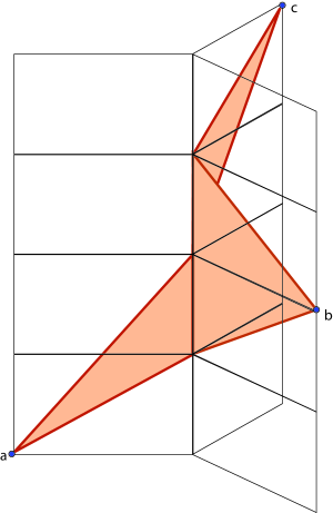
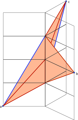
Figure 3: Three points in the open book with three pages. Their geodesic convex hull is shown on the right. The left diagram shows the subset formed by the pairwise geodesics.

We next present a sufficient condition for a set $T$ to be geodesically convex. We regard each orthant $\mathcal{O}_{\sigma}\simeq\mathbb{R}^{d}_{\geq 0}$ as a poset by taking the component-wise partial order.

Theorem 3.5.

Let $\,T$ be a subset of an orthant space $\mathcal{F}_{\Omega}$ such that, for each simplex $\sigma\in\Omega$, the restriction $T_{\sigma}$ is both convex and an order ideal in $\mathcal{O}_{\sigma}$. Then $\,T$ is geodesically convex.

Proof 3.6.

Let $v\in T_{\sigma}$, $w\in T_{\tau}$ and $G(v,w)=[v,u^{1}]\cup[u^{1},u^{2}]\cup\cdots\cup[u^{q},w]$. In order to prove $G(v,w)\subset T$, it suffices to show $u^{i}\in T$ for all $i$, since the restriction of $T$ to each orthant is convex. We first prove $u^{1}\in T$ by constructing a point $u^{*}\in T_{\sigma}$ such that $u^{1}\leq u^{*}$. We let

$$u^{*}\,\,=\,\,\lambda v_{\sigma\backslash A_{1}}+(1-\lambda)w_{\sigma\cap\tau},\;\;\;\text{where}\;\,\,\lambda\,=\,\frac{||w_{B_{1}}||}{||v_{A_{1}}||+||w_{B_{1}}||}.$$

Since the restriction of $T$ to each orthant is an order ideal, we know $v_{\sigma\backslash A_{i}}\leq v\in T_{\sigma}$. We also have $w_{\sigma\cap\tau}\leq w\in T_{\tau}\subset T$ and hence $w_{\sigma\cap\tau}\in T_{\sigma}$. Thus, $u^{*}\in T_{\sigma}$ since $T_{\sigma}$ is convex. By formula (5), $u^{*}_{k}=u^{1}_{k}+(1-\lambda)\frac{||w_{B_{j}}||}{||v_{A_{j}}||}v_{k}$ if $k\in A_{j}$ for some $j=2,\ldots,q$. By formula (4), $u^{*}_{k}=u^{1}_{k}$ if $k\in{\sigma}\backslash(\bigcup_{j=2}^{q}A_{j})$. Since $\lambda\leq 1$, we conclude $u^{1}\leq u^{*}$. This implies $u^{1}\in T_{\sigma}\subset T$. By a similar argument, $u^{i}\in T$ since $u^{i}$ is the first breakpoint of $G(u^{i-1},w)$ for every $i=2,\ldots,q$.

Corollary 3.7.

The compact tree space $\,\mathcal{U}_{m}^{[1]}$ is geodesically convex.

Proof 3.8.

If $T=\mathcal{U}_{m}^{[1]}$ then $T_{\sigma}$ is a subpolytope of the cube $[0,1]^{d}$, with coordinates $\ell_{1},\ldots,\ell_{d}$ as in the end of Section 1. The polytope $T_{\sigma}$ is an order ideal because decreasing the edge lengths in a phylogenetic tree can only decrease the distances between pairs of leaves.

The sufficient condition in Theorem 3.5 is far from necessary. It is generally hard to verify that a set $T$ is geodesically convex, even if $\{T_{\sigma}\}_{\sigma\in\Omega}$ is a polyhedral complex.

Example 3.9 (A Geodesic Triangle).

Let $\Omega$ be the $2$-dimensional flag complex with facets $123$, $234$, $345$ and $456$. We consider eight points in the $3$-dimensional orthant space $\mathcal{F}_{\Omega}\subset\mathbb{R}^{6}$:

$$\begin{matrix}\,\,a=(4,6,6,0,0,0),\,\,b=(0,5,8,0,0,0),\,\,c=(0,0,0,1,2,3),\,\,\,d=(0,0,\frac{1}{7},\frac{5}{7},0,0),\\ e=(0,0,0,\frac{8}{11},\frac{1}{11},0),\,f=(0,0,0,\frac{14}{25},0,0),\,h=(0,\frac{14}{19},\frac{14}{19},0,0,0),\,\,o=(0,0,0,0,0,0).\end{matrix}$$

The geodesic triangle $T={\rm gconv}(a,b,c)$ is a $3$-dimensional polyhedral complex. Its maximal cells are three tetrahedra $T_{123}={\rm conv}\{a,b,h,o\}$, $\,T_{345}={\rm conv}\{d,e,f,o\}$, $T_{456}={\rm conv}\{c,e,f,o\}$, and one bipyramid $T_{234}={\rm conv}\{b,d,f,h,o\}$. These four $3$-polytopes are attached along the triangles $T_{23}={\rm conv}\{b,h,o\}$, $T_{34}={\rm conv}\{d,f,o\}$, and $T_{45}={\rm conv}\{e,f,o\}$.

Verifying this example amounts to a non-trivial computation. We first check that $d,e,f,h,o$ are in the geodesic convex hull of $a,b,c$. This is done by computing geodesic segments as in Section 2. We find $G(a,c)=[a,o]\cup[o,c]$ and $G(b,c)=[b,d]\cup[d,e]\cup[e,c]$. Next, $G(a,e)=[a,x]\cup[x,y]\cup[y,e]$ where $x=(0,\frac{11}{13},\frac{12}{13},0,0,0)$ and $y=(0,0,\frac{6}{67},\frac{44}{67},0,0)$. If we now take $s=\frac{9}{22}b+\frac{13}{22}x$ in $\mathcal{O}_{23}$ then $G(s,c)=[s,f]\cup[f,c]$, and finally $G(a,f)=[a,h]\cup[h,f]$. Now, we need to show that the union of the four $3$-polytopes is geodesically convex. For any two points $v$ and $w$ from distinct polytopes we must show that $G(v,w)$ remains in that union. Here, it does not suffice to take vertices. This is a quantifier elimination problem in piecewise-linear algebra, and we are proud to report that we completed this computation.

The following theorem is the main result in this section.

Theorem 3.10.

Let $d$ be a positive integer. There exists an orthant space of dimension $2d$ and three points in that space such that their geodesic triangle contains a $d$-dimensional simplex.

Proof 3.11.

Fix the simplicial complex $\Omega$ on the vertex set $\{1,2,\ldots,4d\}$ whose $2d+1$ facets are $\{i+1,i+2,\ldots,i+2d\}$ for $i=0,1,\ldots,2d$. This simplicial complex is flag because the minimal non-faces are the $\binom{2d+1}{2}$ pairs $\{i,j\}$ for $j-i\geq 2d$. The corresponding orthant space ${\cal F}_{\Omega}$ has dimension $2d$. We here denote the maximal orthants in ${\cal F}_{\Omega}$ by $\mathcal{O}_{i}={\rm pos}\{e_{i+1},e_{i+2},\ldots,e_{i+2d}\}$.

For each positive integer $i$, we define an integer $v_{i}$ as follows. We set $v_{i}=\frac{i}{2}$ if $i$ is even and $v_{i}=\frac{7(i+1)}{2}$ if $i$ is odd. We fix the points $a=\sum_{i=1}^{2d}v_{i}e_{i}$ and $b=\sum_{i=1}^{2d}e_{i}$ in the first orthant $\mathcal{O}_{0}$ and the point $c=\sum_{i=1}^{2d}e_{2d+i}$ in the last orthant $\mathcal{O}_{2d}$. Explicitly,

$$\begin{array}[]{lll}a&=&(\,7,1,14,2,21,3,28,4,\,\ldots,\,0,0,0,0,0,0,0,0,\ldots),\\ b&=&(\,1,\,1,\,1,\,1,\,1,\,1,\,1,\,1,\,\,\ldots,\,0,0,0,0,0,0,0,0,\ldots),\\ c&=&(\,0,\,0,\,0,\,0,\,0,\,0,\,0,\,0,\,\ldots\,,\,1,1,1,1,1,1,1,1,\,\ldots).\end{array}$$

Consider the geodesic triangle ${\rm gconv}(a,b,c)$ in the orthant space ${\cal F}_{\Omega}$. We shall construct a simplex $P$ of dimension $d$ that is contained in the convex set ${\rm gconv}(a,b,c)\cap\mathcal{O}_{0}$.

We begin with the geodesic segment ${G}(a,c)$. The pair of ordered partitions is

(9) $$\begin{array}[]{lllll}\bigl{(}(\{1,2\},&\{3,4\},&\ldots,&\{2d-1,2d\}),&\\ \;\;(\{2d{+}1,2d{+}2\},&\{2d{+}3,2d{+}4\},&\ldots,&\{4d-1,4d\})\bigr{)}.\end{array}$$

We write the corresponding decompositions into classical line segments as follows:

$$\begin{matrix}G(a,c)&=&[a,u^{1}]\,\cup\,[u^{1},u^{2}]\,\cup\,\cdots\,\cup\,[u^{d-1},u^{d}]\cup[u^{d},c].\\ \end{matrix}$$

Each $u^{i}$, for $1\leq i\leq d$, lies in the relative interior of an orthant of dimension $2d-2$:

$$\begin{matrix}u^{i}~{}\in~{}{\rm pos}\{e_{2i-1},\ldots,e_{2d+2i-2}\}\cap{\rm pos}\{e_{2i+1},\ldots,e_{2d+2i}\}~{}=~{}{\rm pos}\{e_{2i+1},\ldots,e_{2d+2i-2}\}\\ \end{matrix}.$$

We now consider the geodesic segments ${G}(b,u^{i})$ for $i=1,2,\ldots,d$. Let $\widetilde{u}^{i}$ denote the unique intersection point of these geodesic segments with the boundary of $\mathcal{O}_{0}$. Note that $\widetilde{u}^{1}=u^{1}$. The points $a,\widetilde{u}^{1},\ldots,\widetilde{u}^{d}$ lie in the orthant $\mathcal{O}_{0}\simeq\mathbb{R}^{2d}_{\geq 0}$. By construction, they are also contained in the geodesic triangle ${\rm gconv}(a,b,c)$. We shall prove that they are affinely independent.

The above point $u^{i}$ can be written as $\sum_{k=2i-1}^{2d+2i-2}u_{k}^{i}e_{k}$ or as $\sum_{k=2i+1}^{2d+2i}u_{k}^{i}e_{k}$. Note that $u_{k}^{i}=0$ for $k=2i{-}1,2i,2d{+}2i{-}1,2d{+}2i$. For $2i+1\leq k\leq 2d+2i-2$, we claim:

(10) $$u^{i}_{2j-1}~{}=~{}\frac{7(j-i)}{5i+1},\;\;\;\;u^{i}_{2j} = \frac{j-i}{5i+1},\;\;\;\;\text{for}\;i+1\leq j\leq d;\;$$

(11) $$u^{i}_{2d+2j-1}~{}=~{}u^{i}_{2d+2j} = \frac{5(i-j)}{5i+1},\;\;\text{for}\;1\leq j\leq i-1.$$

To prove the above claim, it suffices to verify that the proposed $u^{i}$ satisfy

$$\sum_{i=0}^{d}{d(u^{i},u^{i+1})}~{}=~{}d(a,c),\;\;\text{where}\;u^{0}=a,u^{d+1}=c.$$

In fact, by (3) we have

$$d(a,c)~{}=~{}\sqrt{\sum_{i=1}^{d}{(5i\sqrt{2}+\sqrt{2})^{2}}}~{}=~{}\sqrt{2S_{d}}\qquad\hbox{where}\quad S_{d}=\sum_{i=1}^{d}{(5i+1)^{2}}.$$

For $0\leq i\leq d-1$, we have

$$d(u^{i},u^{i+1}) = \sqrt{\sum_{k=2i+1}^{2d+2i}{(u^{i}_{k}-u^{i+1}_{k})^{2}}}$$

$$= \sqrt{\sum_{j=0}^{d-i-1}{(7^{2}+1^{2})(\frac{j+1}{5i+1}-\frac{j}{5i+6})^{2}}+\sum_{j=0}^{i-1}{2(\frac{5j}{5i+1}-\frac{5j+5}{5i+6})^{2}}}$$

$$= \frac{\sqrt{50}}{(5i+1)(5i+6)}\sqrt{\sum_{j=i+1}^{d}{(5j+1)^{2}}+\sum_{j=1}^{i}{(5j+1)^{2}}}$$

$$= \frac{5}{(5i+1)(5i+6)}\sqrt{2S_{d}}.$$

The sum of these $d$ quantities simplifies to $\,\bigl{(}1-\frac{1}{5d+1}\bigr{)}\sqrt{2S_{d}}$. We next observe that

$$d(u^{d},c) = \sqrt{\sum_{k=2d+1}^{4d}{(u^{d}_{k}-c_{k})^{2}}}~{}=~{}\sqrt{2\sum_{j=0}^{d-1}{(\frac{5j}{5d+1}-1)^{2}}}~{}=~{}\frac{\sqrt{2S_{d}}}{5d+1}.$$

By adding this to the previous sum, we obtain $\sqrt{2S_{d}}=d(a,c)$. So, the claim is proved.

Next, we compute $\widetilde{u}^{i}$ for $1\leq i\leq d$. Recall $\widetilde{u}^{i}$ is the unique intersection point of the geodesic segment ${G}(b,u^{i})$ with ${\rm pos}\{e_{3},\ldots,e_{d}\}$. We note two facts about ${G}(b,u^{i})$:

• The common coordinates of $b$ and $u^{i}$ are $e_{2i-1},\ldots,e_{2d}$.

• By equation (11), the pair of ordered partitions determining $G(b,u^{i})$ is

  $$\begin{array}[]{llllll}\bigl{(}\,(\{1\},&\{2\},&\ldots,&\{2i-2\}),&\\ \;\;\;(\{2d{+}1\},&\{2d{+}2\},&\ldots,&\{2d+2i-2\})\bigr{)}.\end{array}$$

Suppose $\widetilde{u}^{i}=\sum_{k=1}^{2d}\widetilde{u}^{i}_{k}e_{k}$. For $1\leq k\leq 2i-2$, we compute $\widetilde{u}^{i}_{k}$ by (5) and (10). For $2i-1\leq k\leq 2d$, we compute $\widetilde{u}^{i}_{k}$ by (6) and (11). Then we obtain $\widetilde{u}^{i}_{k}$ as follows:

(12) $$\widetilde{u}^{i}_{2j}=\begin{cases}\frac{j+4i-5}{10i-4},&\text{ if }i+1\leq j\leq d;\\ \frac{5j-5}{10i-4},&\text{ if }1\leq j\leq i\\ \end{cases}$$

and

(13) $$\widetilde{u}^{i}_{2j-1}=\begin{cases}\frac{7j-2i-5}{10i-4},&\text{ if }i+1\leq j\leq d;\\ \frac{5j-5}{10i-4},&\text{ if }1\leq j\leq i.\\ \end{cases}$$

The $d+1$ points $\,\widetilde{u}^{0}=a,\widetilde{u}^{1},\ldots,\widetilde{u}^{d}\,$ are contained in $\mathcal{O}_{0}\simeq\mathbb{R}^{2d}$ also in our geodesic triangle. To complete the proof of Theorem 3.10, we will now show that they are affinely independent, so their convex hull is a $d$-simplex. Consider the $(d+1)\times(2d+1)$ matrix $U$, whose $(i+1)$-th row is the vector of homogeneous coordinates of $\widetilde{u}^{i}$. We must show that $U$ has rank $d+1$. Let $U^{\prime}$ be the integer matrix obtained from $U$ by multiplying each row by the denominator $10i-4$. Let $U^{\prime\prime}$ be the $(d+1)\times(d+1)$ submatrix of $U^{\prime}$ formed by the $2,4,\ldots,2d$-th and $(2d+1)$-th columns of $U^{\prime}$. We apply elementary column operators to $U^{\prime\prime}$ to obtain a triangular form. From this, we find that $|\det(U^{\prime\prime})|=4^{d-3}|10d-34|\neq 0$. This means that $U^{\prime\prime}$ has rank $d+1$, and hence so do the rectangular matrices $U^{\prime}$ and $U$.

For an example take $d=5$. The matrix representing $a,\widetilde{u}^{1},\widetilde{u}^{2},\widetilde{u}^{3},\widetilde{u}^{4},\widetilde{u}^{5}$ in $\mathbb{R}^{10}$ is

$$\!\!U~{}=~{}\left[\begin{array}[]{ccccccccccc}7&1&14&2&21&3&28&4&35&5&1\\ \vskip 6.0pt plus 2.0pt minus 2.0pt\cr 0&0&\frac{7}{6}&\frac{1}{6}&\frac{14}{6}&\frac{2}{6}&\frac{21}{6}&\frac{3}{6}&\frac{28}{6}&\frac{4}{6}&1\\ \vskip 6.0pt plus 2.0pt minus 2.0pt\cr 0&0&\frac{5}{16}&\frac{5}{16}&\frac{12}{16}&\frac{6}{16}&\frac{19}{16}&\frac{7}{16}&\frac{26}{16}&\frac{8}{16}&1\\ \vskip 6.0pt plus 2.0pt minus 2.0pt\cr 0&0&\frac{5}{26}&\frac{5}{26}&\frac{10}{26}&\frac{10}{26}&\frac{17}{26}&\frac{11}{26}&\frac{24}{26}&\frac{12}{26}&1\\ \vskip 6.0pt plus 2.0pt minus 2.0pt\cr 0&0&\frac{5}{36}&\frac{5}{36}&\frac{10}{36}&\frac{10}{36}&\frac{15}{36}&\frac{15}{36}&\frac{22}{36}&\frac{16}{36}&1\\ \vskip 6.0pt plus 2.0pt minus 2.0pt\cr 0&0&\frac{5}{46}&\frac{5}{46}&\frac{10}{46}&\frac{10}{46}&\frac{15}{46}&\frac{15}{46}&\frac{20}{46}&\frac{20}{46}&1\end{array}\right]_{6\times 11}.$$

This matrix has rank $6$, so its columns form a $5$-simplex. Hence, the geodesic triangle spanned by the points $a,b,c$ in the orthant space ${\cal F}_{\Omega}$ has dimension at least $5$.

A nice feature of the construction above is that it extends to BHV tree space. The geodesic convex hull of three equidistant trees can have arbitrarily high dimension.

Corollary 3.12.

There exist three ultrametric trees with $2d+2$ leaves whose geodesic triangle in ultrametric BHV space $\mathcal{U}_{2d+2}$ has dimension at least $d$.

Proof 3.13.

Consider the following sequence of $4d$ clades on the set $[2d+2]$. Start with the $2d$ clades $\{1,2\},\{1,2,3\},\{1,2,3,4\},\ldots,\{1,2,3,\ldots,2d+1\}$. Then continue with the $2d$ clades $\{1,3\},\{1,3,4\},\ldots,\{1,3,4,5,\ldots,2d+2\}$. For instance, for $d=5$, our sequence equals

$$\begin{array}[]{ll}&\{1,2\},\{1,2,3\},\{1,2,3,4\},\{1,2,3,4,5\},\dots,\{1,2,3,4,5,6,7,8,9,10,11\},\\ &\{1,3\},\{1,3,4\},\{1,3,4,5\},\{1,3,4,5,6\},\dots,\{1,3,4,5,6,7,8,9,10,11,12\}.\end{array}$$

In this sequence of $4d$ clades, every collection of $2d$ consecutive splits is compatible and forms a trivalent caterpillar tree. No other pair is compatible. Hence the induced subfan of the tree space $\mathcal{U}_{2d+2}$ is identical to the orthant space ${\cal F}_{\Omega}$ in the proof above. The two spaces are isometric. Hence our high-dimensional geodesic triangle exists also in tree space $\mathcal{U}_{2d+2}$.

4 Tropical Convexity

In this section we shift gears, by turning to tropical convexity. We shall assume that the reader is familiar with basics of tropical geometry [19]. We here use the max-plus algebra, so our convention is opposite to that of [19, 24]. The connection between phylogenetic trees and tropical lines, identifying tree space with a tropical Grassmannian, has been explained in many sources, including [19, §4.3] and [24, §3.5]. However, the restriction to ultrametrics [5, §4] offers a fresh perspective. From that vantage point, the discussion of tree mixtures at the end of [24, §3.5] seems to be misleading. We posit here: mixtures of trees are trees!

Let $L_{m}$ denote the cycle space of the complete graph on $m$ nodes with $e:={m\choose 2}$ edges. This is the $(m-1)$-dimensional subspace of $\mathbb{R}^{e}$ defined by the linear equations $\,x_{ij}-x_{ik}+x_{jk}=0\,$ for $1\leq i<j<k\leq m$. The tropicalization of the linear space $L_{m}$ is the set of points $D=(d_{ij})$ such that the following maximum is attained at least twice for all triples $i,j,k$:

$$d_{ij}\oplus d_{ik}\oplus d_{jk}\,=\,{\rm max}(d_{ij},d_{ik},d_{jk}).$$

Disregarding nonnegativity constraints and triangle inequalities, points in ${\rm Trop}(L_{m})$ are precisely the ultrametrics on $[m]$; see [5, Theorem 3] and [19, Example 4.2.14].

As is customary in tropical geometry, we work in the quotient space $\mathbb{R}^{e}/\mathbb{R}{\bf 1}$, where ${\bf 1}=(1,1,\ldots,1)$. The images of ${\rm Trop}(L_{m})$ and $\mathcal{U}_{m}$ in that space are equal. Each point in that image has a unique representative whose coordinates have tropical sum $\,d_{12}\oplus d_{13}\oplus\cdots\oplus d_{m-1,m}={\rm max}(d_{12},d_{13}\ldots,d_{m-1,m})\,$ equal to $1$. Thus, in $\mathbb{R}^{e}/\mathbb{R}{\bf 1}$,

$$\mathcal{U}_{m}^{[1]}\,\,\subset\,\,\mathcal{U}_{m}\,=\,{\rm Trop}(L_{m}).$$

Given two elements $D$ and $D^{\prime}$ in $\mathbb{R}^{e}$, their tropical sum $D\oplus D^{\prime}$ is the coordinate-wise maximum. A subset of $\mathbb{R}^{e}$ is tropically convex if it is closed under the tropical sum operation. The same definitions apply to elements and subsets of $\,\mathbb{R}^{e}/\mathbb{R}{\bf 1}$.

Proposition 4.1.

The tree space $\mathcal{U}_{m}$ is a tropical linear space and is hence tropically convex. The compact tree space $\,\mathcal{U}_{m}^{[1]}$ is a tropically convex subset.

Proof 4.2.

We saw that $\mathcal{U}_{m}={\rm Trop}(L_{m})$ is a tropical linear space, so it is tropically convex by [19, Proposition 5.2.8]. We show that its subset $\mathcal{U}_{m}^{[1]}$ is closed under tropical sums. Suppose two real vectors $a=(a_{1},\ldots,a_{e})$ and $b=(b_{1},\ldots,b_{e})$ satisfy $|a_{i}-a_{j}|\leq 1$ and $|b_{i}-b_{j}|\leq 1$ for all $i,j$. Then the same holds for their tropical sum $a\oplus b$. Indeed, let $a_{i}\oplus b_{i}$ be the largest coordinate of $a\oplus b$ and let $a_{j}\oplus b_{j}$ be the smallest. There are four cases as to which attains the two maxima given by $\oplus$. In all four cases, one easily checks that $|(a_{i}\oplus b_{i})-(a_{j}\oplus b_{j})|\leq 1$.

We briefly recall some basics from tropical convexity [19, §5.2]. A tropical segment is the tropical convex hull ${\rm tconv}(u,v)$ of two points $u=(u_{1}{,}u_{2}{,}\ldots{,}u_{e})$ and $v=(v_{1}{,}v_{2}{,}\ldots{,}v_{e})$ in $\mathbb{R}^{e}/\mathbb{R}{\bf 1}$. It is the concatenation of at most $e-1$ ordinary line segments, with slopes in $\{0,1\}^{e}$. Computing that segment involves sorting the coordinates of $u-v$, so it is done in time $O(e\cdot{\rm log}(e))$. This algorithm is described in the proof of [19, Proposition 5.2.5].

A tropical polytope $\mathcal{P}={\rm tconv}(\mathcal{S})$ is the tropical convex hull of a finite set $\mathcal{S}$ in $\mathbb{R}^{e}/\mathbb{R}{\bf 1}$. This is a classical polyhedral complex of dimension at most $|\mathcal{S}|-1$.

If $\mathcal{D}$ is a real $s\times e$-matrix then the tropical convex hull of its $s$ rows is a tropical polytope in $\mathbb{R}^{e}/\mathbb{R}{\bf 1}$. The tropical convex hull of its $e$ columns is a tropical polytope in $\mathbb{R}^{s}/\mathbb{R}{\bf 1}$. It is a remarkable fact [19, Theorem 5.2.21] that these two tropical polytopes are identical. We write ${\rm tconv}(\mathcal{D})$ for that common object. Example 4.3 illustrates this for a $3{\times}10$-matrix $\mathcal{D}$. Here, ${\rm tconv}(\mathcal{D})$ has dimension $2$ and is shown in Fig. 4.

Example 4.3.

We compute the tropical convex hull ${\rm tconv}(\mathcal{D})$ of the $3\times 10$-matrix

$${\small\mathcal{D}\,\,=\,\,\begin{pmatrix}77/100&1&21/25&1&1&21/25&1&1&13/25&1\\ 1&1&1&1&8/25&3/4&3/4&3/4&3/4&23/50\\ 1&1&1&49/50&16/25&16/25&1&3/100&1&1\end{pmatrix}.}$$

Figure 4: The tropical triangle formed by three equidistant trees on five taxa.

This is the tropical convex hull of the $10$ points in the plane $\mathbb{R}^{3}/\mathbb{R}{\bf 1}$ represented by the column vectors. Its type decomposition is a $2$-dimensional polyhedral complex with $23$ nodes, $35$ edges and $13$ two-dimensional cells. It is shown in Fig. 4. We can also regard ${\rm tconv}(\mathcal{D})$ as a tropical triangle in $\mathbb{R}^{10}/\mathbb{R}{\bf 1}$, namely as the tropical convex hull of the row vectors. The three rows of $\mathcal{D}$ are ultrametrics $(d_{12},d_{13},d_{14},d_{15},d_{23},d_{24},d_{25},d_{34},d_{35},d_{45})$, i.e. points in $\mathcal{U}_{5}$. We denote the three row vectors of the matrix $\mathcal{D}$ by $D^{(1)}$, $D^{(2)}$ and $D^{(3)}$, respectively.

$$\setcounter{MaxMatrixCols}{11}\begin{matrix}d_{12}&d_{13}&d_{14}&d_{15}&d_{23}&d_{24}&d_{25}&d_{34}&d_{35}&d_{45}&{\rm nested}\,\,{\rm set}\\ 77/100&1&21/25&1&1&21/25&1&1&13/25&1&\{12,35,124\}\bullet\\ 21/25&1&21/25&1&1&21/25&1&1&59/100&1&\{35,124\}\\ 1&1&1&1&1&21/25&1&1&3/4&1&\{24,35\}\\ 1&1&1&1&91/100&3/4&91/100&91/100&3/4&91/100&\{24,35,2345\}\\ 1&1&1&1&3/4&3/4&3/4&3/4&3/4&3/4&\{2345\}\\ 1&1&1&1&23/50&3/4&3/4&3/4&3/4&23/50&\{23,45,2345\}\\ 1&1&1&1&8/25&3/4&3/4&3/4&3/4&23/50&\{23,45,2345\}\bullet\\ 1&1&1&1&8/25&3/4&3/4&3/4&3/4&17/25&\{23,45,2345\}\\ 1&1&1&1&39/100&3/4&3/4&3/4&3/4&3/4&\{23,2345\}\\ 1&1&1&1&16/25&3/4&1&3/4&1&1&\{23,234\}\\ 1&1&1&49/50&16/25&73/100&1&73/100&1&1&\{15,23,234\}\\ 1&1&1&49/50&16/25&16/25&1&3/100&1&1&\{15,34,234\}\bullet\\ 1&1&1&49/50&16/25&16/25&1&16/25&1&1&\{15,234\}\\ 1&1&1&49/50&4/5&16/25&1&4/5&1&1&\{15,24,234\}\\ 1&1&1&49/50&89/100&73/100&1&89/100&1&1&\{15,24,234\}\\ 1&1&1&49/50&49/50&41/50&1&49/50&1&1&\{15,24,234\}\\ 1&1&1&1&1&21/25&1&1&1&1&\{24\}\\ 21/25&1&21/25&1&1&21/25&1&1&21/25&1&\{35,124\}\\ 77/100&1&21/25&1&1&21/25&1&1&77/100&1&\{12,35,124\}\vskip 6.0pt plus 2.0pt minus 2.0pt\\ 1&1&1&1&91/100&3/4&91/100&91/100&91/100&91/100&\{24,2345\}\\ 1&1&1&1&91/100&3/4&1&91/100&1&1&\{24,234\}\\ 1&1&1&1&3/4&3/4&1&3/4&1&1&\{234\}\\ 1&1&1&49/50&73/100&73/100&1&73/100&1&1&\{15,234\}\end{matrix}.$$

Table 1: The $23$ ultrametrics (with tree topologies) at the nodes in Fig. 4.

Each of the $23$ nodes in our tropical triangle represents an equidistant tree. In Table 1 we list the $23$ ultrametrics, along with their tree topologies. Those marked with a bullet $\bullet$ are the rows of $\mathcal{D}$. The boundary of ${\rm tconv}(\mathcal{D})$ is given by the first $19$ rows, in counterclockwise order. Rows $1$ to $6$ form the tropical segment from $D^{(1)}$ to $D^{(2)}$, rows $7$ to $12$ form the tropical segment from $D^{(2)}$ to $D^{(3)}$, and rows $13$ to $19$ form the tropical segment from $D^{(3)}$ to $D^{(1)}$. The last four rows are the interior nodes, from top to bottom in Fig. 4. The tropical segment from $D^{(2)}$ to $D^{(3)}$ has depth $1$, but the other two segments have depth $2$. See Section 5 for the definition of “depth”. Note that some of the breakpoints, such as that given in row $6$, lie in the interior of a maximal cone in the tree space $\,\mathcal{U}_{5}={\rm Trop}(L_{5})$. The red circle in Fig. 4 is the tropical centroid, a concept to be introduced in Section 6.

The polyhedral geometry package Polymake [15] can compute the tropical convex hull of a finite set of points. It can also visualize such a tropical polytope, with its cell complex structure, provided its dimension is $2$ or $3$. Fig. 4 was drawn using Polymake.

Matroid theory furnishes the appropriate level of generality for tropical convexity. We refer to the text book reference [19, §4.2] for an introduction. Let $M$ be any matroid of rank $r$ on the ground set $[e]=\{1,2,\ldots,e\}$. The associated tropical linear space ${\rm Trop}(M)$ is a polyhedral fan of dimension $r-1$ in the quotient space $\mathbb{R}^{e}/\mathbb{R}{\bf 1}$. For historical reasons, the tropical linear space ${\rm Trop}(M)$ is also known as the Bergman fan of the matroid $M$; see [3, 5]. The tree space $\mathcal{U}_{m}$ arises when $M$ is the graphic matroid [19, Example 4.2.14] associated with the complete graph $K_{m}$. Here $[e]$ indexes the edges of $K_{m}$, so $e=\binom{m}{2}$ and the rank is $r=m-1$. Fig. 1 (left) shows a rendition of the Petersen graph in [19, Figure 4.1.4].

The tropical linear space ${\rm Trop}(M)$ is tropically convex [19, Proposition 5.2.8]. Hence the notions of tropical segments, tropical triangles, etc. defined above extend immediately to ${\rm Trop}(M)$. This convexity structure on ${\rm Trop}(M)$ is extrinsic and global. It is induced from the ambient space $\mathbb{R}^{e}/\mathbb{R}{\bf 1}$, so it does not rely on choosing a subdivision or local coordinates.

We can also define the structure of an orthant space on ${\rm Trop}(M)$. This requires the choice of a simplicial fan structure on ${\rm Trop}(M)$. Feichtner [11] developed a theory of such fan. Each is determined by a collection of $n$ flats of $M$, known as a building set. From these one constructs a simplicial complex $\Omega$ on $[n]$, known as a nested set complex. This $\Omega$ may or may not be flag. The finest fan structure in this theory arise when all flats of $M$ are in the collection. Here the nested set complex $\Omega$ is flag: it is the order complex of the geometric lattice of $M$. See Exercise 10 in [19, Chapter 4].

Example 4.4.

Let $M$ be the uniform matroid of rank $r$ on $[e]$. The tropical linear space ${\rm Trop}(M)$ is the set of all vectors $u$ in $\mathbb{R}^{e}/\mathbb{R}{\bf 1}$ whose largest coordinate is attained at least $e-r+1$ times. The proper flats of $M$ are the non-empty subsets of $[e]$ having cardinality at most $r-1$. Their number is $n=\sum_{i=1}^{r-1}\binom{e}{i}$. Ordered by inclusion, these form the geometric lattice of $M$. Its order complex is the first barycentric subdivision of the $(r-1)$-skeleton of the $(e-1)$-simplex. This is a flag simplicial complex $\Omega$ with $n$ vertices. The corresponding orthant space $\mathcal{F}_{\Omega}$ in $\mathbb{R}^{n}$ defines the structure of an orthant space on ${\rm Trop}(M)\subset\mathbb{R}^{e}/\mathbb{R}{\bf 1}$.

While the order complex of the geometric lattice of any matroid $M$ makes ${\rm Trop}(M)$ into an orthant space, many matroids have smaller building sets whose nested set complex is flag as well. Our primary example is ultrametric space $\mathcal{U}_{m}={\rm Trop}(L_{m})$. The flats of $L_{m}$ correspond to proper set partitions of $[m]$. Their number is $n=B_{m}{-}2$, where $B_{m}$ is the Bell number. The resulting orthant space on $\mathcal{U}_{m}$ is the $\tau$-space of Gavruskin and Drummond [14]. The subdivision of $\mathcal{U}_{m}$ given by the nested sets of clades is much coarser. It has only $n=2^{m}{-}m{-}2$ rays, and its orthant space gives the BHV metric. This is different from the $\tau$-metric, by [14, Proposition 2]. Note that [14, Figure 4] is the same as our Example 2.6.

Each orthant space structure defines a Euclidean metric on ${\rm Trop}(M)$. These metrics differ dramatically from the tropical metric, to be defined next, in (14). Euclidean metrics on ${\rm Trop}(M)$ are intrinsic and do not extend to the ambient space $\mathbb{R}^{e}/\mathbb{R}{\bf 1}$. Distances are computed by identifying ${\rm Trop}(M)$ with the orthant space $\mathcal{F}_{\Omega}$ of a nested set complex $\Omega$ that is flag. On the other hand, the tropical metric is extrinsic. It lives on $\mathbb{R}^{e}/\mathbb{R}{\bf 1}$ and is defined on ${\rm Trop}(M)$ by restriction. The tropical distance between two points is computed as follows:

(14) $$d_{\rm tr}(v,w)\,\,=\,\,\max\bigl{\{}\,|v_{i}-w_{i}-v_{j}+w_{j}|\,\,:\,\,1\leq i<j\leq e\,\bigr{\}}.$$

This is also known as the generalized Hilbert projective metric [1, §2.2], [10, §3.3]. Unlike in the Euclidean setting of Theorem 2.3, geodesics in that metric are not unique.

Proposition 4.5.

For any two distinct points $v,w\in\mathbb{R}^{e}/\mathbb{R}{\bf 1}$, there are many geodesics between $v$ and $w$ in the tropical metric. One of them is the tropical line segment ${\rm tconv}(v,w)$.

Proof 4.6.

If $u$ is any point whose coordinates lie between those of $v$ and $w$, then $d_{\rm tr}(v,w)=d_{\rm tr}(v,u)+d_{\rm tr}(u,w)$. Hence, any path from $v$ to $w$ that is monotone in each coordinate is a geodesic. One such path is the tropical segment ${\rm tconv}(v,w)$ in the max-plus arithmetic.

One important link between the tropical metric and tropical convexity is the nearest-point map, to be described next. Let $\mathcal{P}$ be any tropically convex closed subset of $\mathbb{R}^{e}/\mathbb{R}{\bf 1}$, and let $u$ be any vector in $\mathbb{R}^{e}$. Let $\mathcal{P}_{\leq u}$ denote the subset of all points in $\mathcal{P}$ that have a representative $v\in\mathbb{R}^{e}$ with $v\leq u$ in the coordinate-wise order. In tropical arithmetic this is expressed as $v\oplus u=u$. If $v$ and $v^{\prime}$ are elements of $\mathcal{P}_{\leq u}$ then so is their tropical sum $v\oplus v^{\prime}$. It follows that $\mathcal{P}_{\leq u}$ contains a unique coordinate-wise maximal element, denoted ${\rm max}(\mathcal{P}_{\leq u})$.

Theorem 4.7.

Given any tropically convex closed subset $\mathcal{P}$ of $\,\mathbb{R}^{e}/\mathbb{R}{\bf 1}$, consider the function

(15) $$\pi_{\mathcal{P}}\,:\,\mathbb{R}^{e}/\mathbb{R}{\bf 1}\rightarrow\mathcal{P}\,,\,\,u\mapsto{\rm max}(\mathcal{P}_{\leq u}).$$

Then $\pi_{\mathcal{P}}(u)$ is the unique point in $\mathcal{P}$ that minimizes the tropical distance to $u$.

This result was proved by Cohen, Gaubert and Quadrat in [10, Theorem 18]. See also [1]. In Section 6 we shall discuss the important case when $\mathcal{P}={\rm Trop}(M)$ is a tropical linear space. The subcase when $\mathcal{P}$ is a tropical hyperplane appears in [1, §7].

We close this section by considering a tropical polytope, ${\rm tconv}(D^{(1)},D^{(2)},\ldots,D^{(s)})$. The $D^{(i)}$ are points in $\mathbb{R}^{e}/\mathbb{R}{\bf 1}$. For instance, they might be ultrametrics in $\mathcal{U}_{m}$. Then

$$\pi_{\mathcal{P}}(D)\,=\,\lambda_{1}\odot D^{(1)}\,\oplus\,\lambda_{2}\odot D^{(2)}\,\oplus\,\cdots\,\oplus\,\lambda_{s}\odot D^{(s)},\quad{\rm where}\,\,\lambda_{k}={\rm min}(D-D^{(k)}).$$

This formula appears in [19, (5.2.3)]. It allows us to easily project an ultrametric $D$ (or any other point in $\mathbb{R}^{e}$) onto the tropical convex hull of $s$ given ultrametrics.

5 Experiments with Depth

It is natural to compare tropical convexity with geodesic convexity. One starts by comparing the line segments ${\rm gconv}(v,w)$ and ${\rm tconv}(v,w)$, where $v,w$ are points in a tropical linear space ${\rm Trop}(M)$. Our first observation is that tropical segments generally do not obey the combinatorial structure imposed by ordered partitions $(\mathcal{A},\mathcal{B})$. For instance, if $v$ and $w$ represent equidistant trees then every clade used by a tree in the geodesic segment ${\rm gconv}(v,w)$ must be a clade of $v$ or $w$. This need not hold for trees in the tropical segment ${\rm tconv}(v,w)$.

Example 5.1.

Let $v=D^{(1)}$ and $w=D^{(2)}$ in Example 4.3. Their tree topologies are given by the sets of clades $\{12,35,124\}$ and $\{23,45,2345\}$. Consider the breakpoints of the tropical segment ${\rm tconv}(v,w)$ given in lines 3 and 4 of Table 1. Both trees have the new clade $24$.

This example suggests that tropical segments might be worse than Euclidean geodesics. However, as we shall now argue, the opposite is the case: for us, tropical segments are better. We propose the following quality measure for a path $P$ in an orthant space $\mathcal{F}_{\Omega}$. Suppose that $\mathcal{F}_{\Omega}$ has dimension $d$. Each point of $P$ lies in the relative interior of a unique orthant $\mathcal{O}_{\sigma}$, and we say that this point has codimension $d-{\rm dim}(\mathcal{O}_{\sigma})$. We define the depth of a path $P$ as the maximal codimension of any point in $P$. For instance, the depth of the Euclidean geodesic in Theorem 2.3 is the maximum of the numbers $\sum\limits_{k=1}^{i}|A_{k}|-\sum\limits_{k=1}^{i-1}|B_{k}|$, where $i$ runs over $\{1,2,\ldots,q\}$. These are the codimensions of the breakpoints of ${\rm gconv}(v,w)$.

Geodesics of small depth are desirable. A cone path has depth $d$. Cone paths are bad from a statistical perspective because they give rise to sticky means, see e.g. [16], [20] or [21, §5.3]. Optimal geodesics have depth $0$. Such geodesics are line segments within a single orthant. These occur if and only if the starting point and target point are in the same orthant. If the two given points are not in the same orthant then the best-case scenario is depth $1$, which means that each transition is through an orthant of codimension $1$ in $\mathcal{F}_{\Omega}$. We conducted two experiments, to assess the depths of ${\rm gconv}(v,w)$ and ${\rm tconv}(v,w)$.

Experiment 5.2 (Euclidean Geodesics).

For each $m\in\{4,5,\ldots,20\}$, we sampled $1000$ pairs $\{v,w\}$ from the compact tree space $\mathcal{U}_{m}^{[1]}$, and for each pair we computed the depth of ${\rm gconv}(v,w)$. The sampling scheme is described below. The depths are integers between $0$ and $m-2$.

Algorithm 5.3 (Sampling normalized equidistant trees with $m$ leaves).

Input: The number $m$ of leaves, and the sample size $s$.
Output: A sample of $s$ random equidistant trees in the compact tree space $\,\mathcal{U}_{m}^{[1]}$.

1. Set $\mathcal{S}=\emptyset$.

2. For $i=1,\ldots s$, do

   1. Generate a tree $D_{i}$ using the function rcoal from the ape package [25] in R.

   2. Randomly permute the leaf labels on the metric tree $D_{i}$.

   3. Change the clade nested structure of $D_{i}$ by randomly applying the nearest neighbor interchange (NNI) operation $m$ times.

   4. Turn $D_{i}$ into an equidistant tree using the ape function compute.brtime.

   5. Normalize $U_{i}$ so that the distance from the root to each leaf is $\frac{1}{2}$.

   6. Add $D_{i}$ to the output set $\mathcal{S}$.

3. Return $\mathcal{S}$.

Table 2 shows the distribution of the depths. For instance, the first row concerns $1000$ random geodesics on the $2$-dimensional polyhedral fan $\mathcal{U}_{4}$ depicted in Fig. 1. Of these geodesics, $8.4\%$ were in a single orthant, $58.4\%$ had depth $1$, and $33.2\%$ were cone paths. For $m=20$, the fraction of cone paths was $6.2\%$. The data in Table 2 are based on the sampling scheme in Algorithm 5.3.

$\!\!m\backslash$depth ​​​​​	0	1	2	3	4	5	6	7	8	9	10	11	12	13	14	15	16	​​17​​	​​18​​
4	8.4	​​​​​ 58.4 ​​​​​	​​​​ 33.2 ​​​​
5	1.6	​​​​​ 26.4 ​​​​​	​​​​ 47.4 ​​​​	​​​​ 24.6 ​​​​
6	0.2	​​​​ ​13.2 ​​​​​	​​​​ 36.7 ​​​​	​​​​ 31.5 ​​​​	​​​​ 18.4 ​​​​
7	0	4	​​​​ ​25.9​ ​​​​	​​​​ 29.9 ​​​​	​​​​ 22.2 ​​​​	18
8	0	1.1	15	​​28.9​​	25	​​17.1​​	​​12.9​​
9	0	0.8	8	​​22.1​​	​​25.9​​	​​18.3​​	​​14.5​​	​​10.4​​
10	0	0.4	3.3	​​17.2​​	​​22.3​​	​​20.6​​	​​14.1​​	​​13.2​​	8.9
11	0	0.2	1.5	​​10.4​​	​​17.6​​	​​20.3​​	​​16.8​​	​​12.8​​	​​11.1​​	9.3
12	0	0.2	0.1	6	​​14.1​​	​​20.4​​	​​13.9​​	​​14.6​​	​​12.7​​	​​10.5​​	7.5
13	0	0.2	0.4	4.2	10.1	17.2	15.9	12.5	11	9.8	9.1	9.6
14	0	0.2	0	2.7	9.3	14.9	15.5	12.2	11.3	​​10.4​​	8.7	8	6.8
15	0	0.1	0	1.4	5.9	12.7	13	13.1	11.3	9.2	8.9	8.5	7.5	8.4
16	0	0	0	1	5	11.2	11.4	11.3	11.2	9.9	8.1	9.1	7.3	6.7	7.8
17	0	0	0	0.2	3.4	5.9	10.7	11	11.2	​​11.5 ​​	8.4	7.9	7.9	6.2	8.5	7.2
18	0	0	0.1	0.4	1.5	6.5	8.7	10.5	10.9	9.7	7.9	7.5	7.1	8.7	7.7	6.5	6.3
19	0	0	0	0.2	1.6	5	7.2	9.3	9.6	8.5	7.5	8.3	7.4	6.1	9.2	7.4	6.8	​​​5.9​​​
20	0	0	0	0	0.5	3	6.7	7.6	11.2	9.8	9.4	8.2	5.9	7.5	6.9	6.9	4.5	​​​5.7​​​	​​​​​6.2​​​​​

Table 2: The rows are labeled by the number $m$ of taxa and the columns are labeled by the possible depths of a geodesic in tree space. The entries in each row sum to $100\%$. They are the frequencies of the depths among $1000$ geodesics, randomly sampled using Algorithm 5.3.

Next we perform our experiment with the tropical line segments ${\rm tconv}(v,w)$.

Experiment 5.4 (Tropical Segments).

For each $m\in\{4,5,\ldots,20\}$, we revisited the same $1000$ pairs $\{v,w\}$ from Experiment 5.2, and we computed their tropical segments ${\rm tconv}(v,w)$. Table 3 shows the distribution of their depths.

$m\backslash$depth​​	0	1	2	3	4	5	6	7	8	9	10
4	8.1	88.7	3.2
5	1.5	84.7	13.8	0
6	0.3	69.9	29.8	0	0
7	0	55.7	44.1	0.2	0	0
8	0	42.8	56.9	0.2	0.1	0	0
9	0	28.0	71.4	0.6	0	0	0	0
10	0	20.7	78.2	1.1	0	0	0	0	0
11	0	10.8	88.0	1.1	0.1	0	0	0	0	0
12	0	7.8	89.5	2.4	0.2	0.1	0	0	0	0	0
13	0	5.3	90.8	3.5	0.3	0.1	0	0	0	0	0
14	0	2.5	92.1	4.9	0.5	0	0	0	0	0	0
15	0	1.9	90.4	6.8	0.9	0	0	0	0	0	0
16	0	0.4	88.7	9.4	1.1	0.4	0	0	0	0	0
17	0	0.8	87.5	9.4	2.3	0	0	0	0	0	0
18	0	0.8	86.1	9.7	3.1	0.2	0	0.1	0	0	0
19	0	0.3	84.1	11.3	3.4	0.8	0.1	0	0	0	0
20	0	0.1	78.4	16.5	3.9	1.0	0	0.1	0	0	0

Table 3: Frequencies of the depths among $1000$ tropical segments. The same input data as in Table 2 was used.

There is a dramatic difference between Tables 2 and 3. The depths of the Euclidean geodesics are much larger than those of the tropical segments. Since small depth is desirable, this suggests that the tropical convexity structure may have good statistical properties.

Triangles show even more striking differences: While tropical triangles ${\rm tconv}(a,b,c)$ are $2$-dimensional, geodesic triangles ${\rm gconv}(a,b,c)$ can have arbitrarily high dimension, by Theorem 3.10. In spite of these dimensional differences, $\,{\rm tconv}(a,b,c)\,$ is usually not contained in $\,{\rm gconv}(a,b,c)$. In particular, this is the case in the following example.

Example 5.5.

Fix $e=4,r=3$ and let $M$ be the matroid with bases $124,134,234$. The tropical plane ${\rm Trop}(M)$ is defined in $\mathbb{R}^{4}/\mathbb{R}{\bf 1}$ by $x_{1}\oplus x_{2}\oplus x_{3}$. Geometrically, this is the open book with three pages in Example 3.4. The following points lie in ${\rm Trop}(M)$:

$$a=(0,1,1,2),\quad b=(1,0,1,4),\quad c=(1,1,0,6).$$

Fig. 5 shows the two triangles ${\rm gconv}(a,b,c)$ and ${\rm tconv}(a,b,c)$ inside that open book. See Example 3.4 and Fig. 3 for the derivation of the geodesic triangle.

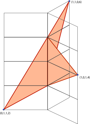
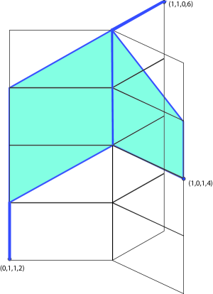
Figure 5: Two convex hulls of three points $a,b,c$ inside the open book with three pages. The geodesic triangle is shown on the left, while the tropical triangle is on the right.

6 Towards Tropical Statistics

Geometric statistics is concerned with the analysis of data sampled from highly non-Euclidean spaces [16, 20]. The section title above is meant to suggest the possibility that objects and methods from tropical geometry can play a role in this development. As an illustration consider the widely used technique of Principal Component Analysis (PCA). This serves to reduce the dimension of high-dimensional data sets, by projecting these onto lower-dimensional subspaces in the data space. The geometry of dimension reduction is essential in phylogenomics, where it can provide insight into relationships and evolutionary patterns of a diversity of organisms, from humans, plants and animals, to microbes and viruses.

To see how tropical convexity might come in, consider the work of Nye [22] in statistical phylogenetics. Nye developed PCA for BHV tree space. We identify tree space with $\mathcal{U}_{m}$ and we sketch the basic ideas. Nye defined a line $L$ in $\mathcal{U}_{m}$ to be an unbounded path such that every bounded subpath is a BHV geodesic. Suppose that $L$ is such a line, and $u\in\mathcal{U}_{m}\backslash L$. Proposition 2.1 in [22] shows that $L$ contains a unique point $x$ that is closest to $u$ in the BHV metric. We call $x$ the projection of $u$ onto the line $L$. Given $u$ and $L$, we can compute $x$ as follows. Fixing a base point $L(0)$ on the line, one choses a geodesic parametrization $L(t)$ of the line. This means that $t$ is the distance $d(L(0),L(t))$. Also let $k$ denote the distance from $u$ to $L(0)$. By the triangle inequality, the desired point is $x=L(t^{*})$ for some $t^{*}\in[-k,k]$. The distance $d(x,L(t))$ is a continuous function of $t$. Our task is to find the value of $t^{*}$ which minimizes that function on the closed interval $[-k,k]$. This is done using numerical methods. The uniqueness of $t^{*}$ follows from the ${\rm CAT}(0)$ property.

Suppose we are given a collection $\{v^{1},v^{2},\ldots,v^{s}\}$ of tree metrics on $m$ taxa. This is our data set for phylogenetic analysis. Nye’s method computes a first principal line (regression line) for these data inside BHV space. This is done as follows. One first computes the centroid $x^{0}$ of the $s$ given trees. This can be done using the iterative method in [7, Theorem 4.1]. Now, the desired regression line $L$ is one of geodesics through $x^{0}$. For any such line $L$, we can compute the projections $x^{1},\ldots,x^{s}$ of the data points $v^{1},\ldots,v^{s}$. The goal is to find the line $L$ that minimizes (or, maximizes) a certain objective function. Nye proposes two such functions:

$$f_{\perp}(L):=\sum_{i=1}^{s}d(v^{i},x^{i})^{2}\quad\hbox{or}\quad f_{\|}(L):=\sum_{i=1}^{s}d(x^{0},x^{i})^{2}.$$

The first function of $L$ above can be minimized and the second function above can be maximized using an iterative numerical procedure.

While the paper [22] represents a milestone concerning statistical inference in BHV tree space, it left the open problem of computing higher-dimensional principal components. First, what are geodesic planes? Which of them is the regression plane for $v^{1},v^{2},\ldots,v^{s}$? Ideally, a plane in tree space would be a $2$-dimensional complex that contains the geodesic triangle formed by any three of its points. Outside a single orthant, do such planes even exist? Such questions were raised in [22, §6]. Our Theorem 3.10 suggests that the answer is negative.

On the other hand, tropical convexity and tropical linear algebra in $\mathcal{U}_{m}$ behave better. Indeed, each triangle ${\rm tconv}(v^{1},v^{2},v^{3})$ in $\mathbb{R}^{e}\!/\mathbb{R}{\bf 1}$ is $2$-dimensional and spans a tropical plane; each tropical tetrahedron ${\rm tconv}(v^{1},v^{2},v^{3},v^{4})$ is $3$-dimensional and spans a tropical $3$-space. These tropical linear spaces are best represented by their Plücker coordinates; cf. [19, §4.4].

In what follows we take first steps towards the introduction of tropical methods into geometric statistics. We study tropical centroids and projections onto tropical linear spaces.

In any metric space $\mathcal{M}$, one can study two types of “centroids”: one is the Fréchet mean and the other is the Fermat-Weber point. Given a finite sample $\{v^{1},v^{2},\ldots,v^{s}\}$ of points in $\mathcal{M}$, a Fréchet mean minimizes the sum of squared distances to the points. A Fermat-Weber point $y$ minimizes the sum of distances to the given points.

(16) $$y\,:=\,\operatorname*{arg\,min}_{z\in\mathcal{M}}\sum_{i=1}^{s}d(z,v^{i}).$$

Here we do not take the square. We note that $y$ is generally not a unique point but refers to the set of all minimizers. Millar et.al. [21] took the Fréchet mean for the centroid in orthant spaces. In the non-Euclidean context of tropical geometry, we prefer to work with the Fermat-Weber points. If $v^{1},\ldots,v^{s}\in\mathcal{M}\subset\mathbb{R}^{e}/\mathbb{R}{\bf 1}$ then a tropical centroid is any solution $y$ to (16) with $d=d_{\rm tr}$. In unconstrained cases, we can use the following linear program to compute tropical centroids:

Proposition 6.1.

Suppose $\mathcal{M}=\mathbb{R}^{e}/\mathbb{R}{\bf 1}$. Then the set of tropical centroids is a convex polytope. It consists of all optimal solutions $y=(y_{1},\ldots,y_{e})$ to the following linear program:

(17) $$\begin{matrix}{\rm minimize}\quad d_{1}+d_{2}+\cdots+d_{s}\quad\hbox{\rm subject to}\qquad\qquad\qquad\\ \qquad\qquad y_{j}-y_{k}-v^{i}_{j}+v^{i}_{k}\geq-d_{i}\quad\hbox{for all}\,\,\,i=1,\ldots,s\,\,\hbox{and}\,\,\,1\leq j,k\leq e,\\ \qquad\qquad y_{j}-y_{k}-v^{i}_{j}+v^{i}_{k}\leq\phantom{-}d_{i}\quad\hbox{for all}\,\,\,i=1,\ldots,s\,\,\hbox{and}\,\,\,1\leq j,k\leq e.\end{matrix}$$

We refer to the subsequent paper [18] for details, proofs, and further results on the topic discussed here. If $\mathcal{M}$ is a proper subset of $\mathbb{R}^{e}/\mathbb{R}{\bf 1}$ then the computation of tropical centroids is highly dependent on the representation of $\mathcal{M}$. For tropical linear spaces, $\mathcal{M}={\rm Trop}(M)$, we must solve a linear program on each maximal cone. The question remains how to do this efficiently.

Example 6.2.

Consider the rows of the $3\times 10$-matrix in Example 4.3. We compute the tropical centroid of these three points in $\mathcal{M}=\mathcal{U}_{5}\subset\mathbb{R}^{10}/\mathbb{R}{\bf 1}$. To do this, we first compute the set of all tropical centroids in $\mathbb{R}^{10}/\mathbb{R}{\bf 1}$. This is a $6$-dimensional classical polytope, consisting of all optimal solutions to (17). The intersection of that polytope with tree space $\mathcal{U}_{5}$ equals the parallelogram

$$\begin{matrix}\bigl{\{}\left(1,1,1,1,\frac{61}{100}{+}y,\frac{61}{100}{+}x{+}y,\frac{3}{4}+y,\frac{61}{100}{+}y,\frac{3}{4}{+}y,\frac{3}{4}{+}y\right):0\leq x\leq\frac{43}{100},\,0\leq y\leq\frac{7}{50}\bigr{\}}.\end{matrix}$$

This is mapped to a single (red) point inside the tropical triangle in Fig. 4.

Example 6.2 shows that tropical centroids of a finite set of points generally do not lie in the tropical convex hull of those points. For instance, the tropical centroid of $\{D^{(1)},D^{(2)},D^{(3)}\}$ that is obtained by setting $x=y=0$ in the parallelogram above does not lie in ${\rm tconv}(D^{(1)},D^{(2)},D^{(3)})$.

We now come to our second and last topic in this section, namely projecting onto subspaces. Let $L_{\bf w}$ be a tropical linear space of dimension $r-1$ in $\mathbb{R}^{e}/\mathbb{R}{\bf 1}$. This concept is to be understood in the inclusive sense of [19, Definition 4.4.3]. The notation $L_{\bf w}$ also comes from [19]. Hence ${\bf w}=(w_{\sigma})$ is a vector in $\mathbb{R}^{\binom{e}{r}}$ that lies in the Dressian $\,{\rm Dr}(r,e)$, as in [19, Definition 4.4.1]. The Plücker coordinates $w_{\sigma}$ are indexed by subsets $\sigma\in\binom{[e]}{r}$. Among the $L_{\bf w}$ are the tropicalized linear spaces [19, Theorem 4.3.17]. Even more special are linear spaces spanned by $r$ points; cf. [12]. If $L_{\bf w}$ is spanned by $x^{1},\ldots,x^{r}$ in $\mathbb{R}^{e}/\mathbb{R}{\bf 1}$ then its Plücker coordinate $w_{\sigma}$ is the tropical determinant of the $r\times r$-submatrix indexed by $\sigma$ of the $r\times e$-matrix $X=(x^{1},\ldots,x^{e})$. Note that all tropical linear spaces $L_{\bf w}$ are tropically convex.

We are interested in the nearest point map $\pi_{L_{\bf w}}$ that takes a point $u$ to the largest point in $L_{\bf w}$ dominated by $u$, as seen in (15). From [17, Theorem 15] we have:

Theorem 6.3 (The Blue Rule).

The $i$-th coordinate of the point in $L_{\bf w}$ nearest to $u$ is equal to

(18) $$\quad\pi_{L_{\bf w}}(u)_{i}\,\,=\,\,{\rm max}_{\tau}\,{\rm min}_{j\not\in\tau}\bigl{(}u_{j}+w_{\tau\cup i}-w_{\tau\cup j}\bigr{)}\qquad{\rm for}\,\,\,i=1,2,\ldots,e.$$

Here $\tau$ runs over all $(r-1)$-subsets of $[e]$ that do not contain $i$.

The special case of this theorem when $L_{\bf w}$ has the form ${\rm Trop}(M)$, for some rank $r$ matroid $M$ on $[e]$, was proved by Ardila in [3, Theorem 1]. Matroids correspond to the case when each tropical Plücker coordinate $w_{\sigma}$ is either $0$ or $-\infty$. The application that motivated Ardila’s study was the ultrametric tree space $\mathcal{U}_{m}$. Here the nearest-point map computes the largest ultrametric dominated by a given dissimilarity map, a problem of importance in phylogenetics. An efficient algorithm for this problem was given by Chepoi and Fichet [9]. This was recently revisited by Apostolico et al. in [2].

Example 6.4.

Following Example 4.4, let $M$ be the uniform matroid of rank $r$ on $[e]$. Then ${\rm Trop}(M)=L_{\bf w}$ where ${\bf w}$ is the all-zero vector, i.e. $w_{\sigma}=0$ for $\sigma\in\binom{[e]}{r}$. By (18), the $i$-th coordinate of the nearest point $\pi_{L_{\bf w}}(u)$ equals $\,{\rm max}_{\tau}\,{\rm min}_{j\not\in\tau}u_{j}$. That nearest point is obtained from $u$ by replacing the $e-r$ largest coordinates in $u$ by the $r$-th smallest coordinate.

Returning to ideas for geometric statistics, the Blue Rule may serve as a subroutine for the numerical computation of regression planes. Let $u^{1},\ldots,u^{s}$ be data points in $\mathbb{R}^{e}/\mathbb{R}{\bf 1}$, lying in a tropically convex subset $\mathcal{P}$ of interest, such as $\mathcal{P}=\mathcal{U}_{m}$. The tropical regression plane of dimension $r-1$ is a solution to the optimization problem

(19) $$\operatorname*{arg\,min}_{L_{\bf w}}\sum_{i=1}^{s}d_{\rm tr}(u^{i},L_{\bf w}).$$

Here ${\bf w}$ runs over all points in the Dressian ${\rm Dr}(r,e)$, or in the tropical Grassmannian ${\rm Gr}(r,e)$. One might restrict to Stiefel tropical linear spaces [12], i.e. those that are spanned by points. Even the smallest case $r=2$ is of considerable interest, as seen in the study of Nye [22]. In his approach, we would first compute the tropical centroid inside $\mathcal{P}$ of the sample $\{u^{1},u^{2},\ldots,u^{s}\}$. Fix $x^{1}$ to be that centroid. Now $x^{2}\in\mathcal{P}$ is the remaining decision variable, and we optimize over all tropical lines spanned by $x^{1}$ and $x^{2}$ inside $\mathbb{R}^{e}/\mathbb{R}{\bf 1}$. Such a line is a tree with $e$ unbounded rays. If the ambient tropically convex set $\mathcal{P}$ is a tropical linear space, such as our tree space $\mathcal{U}_{m}$, then the regression tree $L_{\bf w}$ will always be contained inside $\mathcal{P}$.

Acknowledgements. We thank Simon Hampe, Andrew Francis and Megan Owen for helpful conversations. This project started in the summer of 2015, when all authors were hosted by the National Institute for Mathematical Sciences, Daejeon, Korea. Ruriko Yoshida was supported by travel funds from the Department of Statistics in the College of Arts and Sciences at the University of Kentucky. Bernd Sturmfels thanks the US National Science Foundation (DMS-1419018) and the Einstein Foundation Berlin.

References

- [1] M. Akian, S. Gaubert, N. Viorel and I. Singer, Best approximation in max-plus semimodules, Linear Algebra Appl. 435 (2011), pp. 3261–3296.
- [2] A. Apostolico, M. Comin, A. Dress and L. Parida, Ultrametric networks: a new tool for phylogenetic analysis, Algorithms for Molecular Biology 8 (2013), pp. 7.
- [3] F. Ardila, Subdominant matroid ultrametrics, Annals of Combinatorics 8 (2004), pp. 379–389.
- [4] F. Ardila, T. Baker and R. Yatchak, Moving robots efficiently using the combinatorics of CAT(0) cubical complexes, SIAM J. Discrete Math. 28 (2014), pp. 986–1007.
- [5] F. Ardila and C. Klivans, The Bergman complex of a matroid and phylogenetic trees, Journal of Combinatorial Theory Ser. B 96 (2006), pp. 38–49.
- [6] M. Berger, A Panoramic View of Riemannian Geometry, Springer Verlag, Berlin, 2003.
- [7] L. Billera, S. Holmes and K. Vogtman, Geometry of the space of phylogenetic trees, Advances in Applied Mathematics 27 (2001), pp. 733–767.
- [8] B. Bowditch, Some results on the geometry of convex hulls in manifolds of pinched negative curvature, Comment. Math. Helvetici 69 (1994), pp. 49–81.
- [9] V. Chepoi and B. Fichet, approximation via subdominants, Journal of Mathematical Psychology 44 (2000), pp. 600–616.
- [10] G. Cohen, S. Gaubert and J.P. Quadrat, Duality and separation theorems in idempotent semimodules, Linear Algebra Appl. 379 (2004), pp. 395–422.
- [11] E. Feichtner, Complexes of trees and nested set complexes, Pacific Journal of Mathematics 227 (2006), pp. 271–286.
- [12] A. Fink and F. Rincón, Stiefel tropical linear spaces, J. Combin. Theory A 135 (2015), pp. 291–331.
- [13] P.T. Fletcher, J. Moeller, J.M. Phillips and S. Venkatasubramanian, Computing hulls, centerpoints and VC dimension in positive definite spaces, presented at Algorithms and Data Structures Symposium, New York, 2011; original version at arXiv:0912.1580.
- [14] A. Gavruskin and A. Drummond, The space of ultrametric phylogenetic trees, Journal of Theoretical Biology 403 (2016), pp. 197–208.
- [15] E. Gawrilow and M. Joswig, polymake: a framework for analyzing convex polytopes, in Polytopes: combinatorics and computation, 43–73, DMV Seminar 29, Birkhäuser, Basel, 2000.
- [16] T. Hotz, S. Huckemann, H. Le, J. Marron, J. Mattingly, E. Miller, J. Nolen, M. Owen, V. Patrangenaru and S. Skwerer, Sticky central limit theorems on open books, Annals of Applied Probability 6 (2013), pp. 2238–2258.
- [17] M. Joswig, B. Sturmfels and J. Yu, Affine buildings and tropical convexity, Albanian J. Math. 1 (2007), pp. 187–211.
- [18] B. Lin and R. Yoshida, Tropical Fermat-Weber points, arXiv:1604.04674.
- [19] D. Maclagan and B. Sturmfels, Introduction to Tropical Geometry, Graduate Studies in Mathematics, 161, American Mathematical Society, Providence, RI, 2015.
- [20] E. Miller, Fruit flies and moduli: Interactions between biology and mathematics, Notices of the American Mathematical Society 62(10) (2015), pp. 1178–1183.
- [21] E. Miller, M. Owen and S. Provan, Polyhedral computational geometry for averaging metric phylogenetic trees, Advances in Applied Mathematics 68 (2015) pp. 51–91.
- [22] T. Nye, Principal components analysis in the space of phylogenetic trees, Annals of Statistics 39 (2011), pp. 2716–2739.
- [23] M. Owen and S. Provan, A fast algorithm for computing geodesic distances in tree space, IEEE/ACM Trans. Computational Biology and Bioinformatics 8 (2011), pp. 2–13.
- [24] L. Pachter and B. Sturmfels, Algebraic Statistics for Computational Biology, Cambridge University Press, 2005.
- [25] E. Paradis, J. Claude and K. Strimmer, APE: analyses of phylogenetics and evolution in R language, Bioinformatics 20 (2004), pp. 289–290.
- [26] C. Semple and M. Steel, Phylogenetics, Oxford Lecture Series in Mathematics and its Applications, 24, Oxford University Press, 2003.