Maximum Likelihood Foreground Cleaning for Cosmic Microwave Background Polarimeters in the Presence of Systematic Effects

Abstract

We extend a general maximum likelihood foreground estimation for cosmic microwave background polarization data to include estimation of instrumental systematic effects. We focus on two particular effects: frequency band measurement uncertainty, and instrumentally induced frequency dependent polarization rotation. We assess the bias induced on the estimation of the $B$-mode polarization signal by these two systematic effects in the presence of instrumental noise and uncertainties in the polarization and spectral index of Galactic dust. Degeneracies between uncertainties in the band and polarization angle calibration measurements and in the dust spectral index and polarization increase the uncertainty in the extracted CMB $B$-mode power, and may give rise to a biased estimate. We provide a quantitative assessment of the potential bias and increased uncertainty in an example experimental configuration. For example, we find that with 10% polarized dust, tensor to scalar ratio of $r=0.05$, and the instrumental configuration of the EBEX balloon payload, the estimated CMB $B$-mode power spectrum is recovered without bias when the frequency band measurement has 5% uncertainty or less, and the polarization angle calibration has an uncertainty of up to 4^∘.

1 Introduction

The inflationary paradigm posits that the universe underwent a period of exponential expansion within its first fraction of a second. One of the generic predictions of inflation is the production of stochastic gravitational wave background and the imprint of a $B$-mode pattern in the polarization of the cosmic microwave background (CMB) radiation on large angular scales (Kamionkowski et al., 1997; Seljak & Zaldarriaga, 1997). The level of the inflationary gravitational wave $B$-mode signal encodes information about the inflationary energy scale and is characterized by a tensor-to-scalar ratio $r$ which quantifies the relative strength of gravity waves and density perturbations produced during inflation. The current upper limit from $B$-mode observation alone is $r<0.12$ (BICEP2/Keck and Planck Collaborations, 2015; Planck Collaboration, 2015a). On small angular scales there is more dominant source of $B$-mode polarization: lensing of CMB photons by the large scale structure of the universe, which converts CMB $E$-mode to $B$-mode (Zaldarriaga & Seljak, 1998).

According to recent observations, polarized Galactic thermal dust emission is a significant source of contamination for the inflationary $B$-mode signal (Gold et al., 2009; Fraisse et al., 2013; Planck Collaboration, 2014; BICEP2/Keck and Planck Collaborations, 2015). To monitor and subtract Galactic foreground contamination many CMB polarimeters observe at multiple frequency bands. In this paper we address foreground estimation for CMB polarimeters in the presence of two systematic effects: uncertainty in measurement of the frequency band, and frequency dependent polarization rotation.

Band measurement uncertainty is a common systematic effect. Absolute calibration uncertainty, which affects all signal components within a given frequency band by the same factor, has already been discussed in Stompor et al. (2009), Stivoli et al. (2010) and Errard & Stompor (2012). In this paper we focus on band measurement uncertainty, which affects sky signals with different emission spectra differently. In the context of foreground estimation with unknown foreground spectral parameters, the effect of band measurement uncertainties has not yet been studied much in detail. Church et al. (2003) gave an analytic calculation of the effect of error in the knowledge of bands given sky signals with fixed and known spectral shape. Bao et al. (2012) studied the impact of band measurement uncertainty in the presence of an achromatic half-wave plate (AHWP) and proposed an approximate dust estimation and subtraction process.

For CMB polarimeters using an AHWP, such as the E and B experiment (EBEX) (Reichborn-Kjennerud et al., 2010), or using a sinuous antenna multi-chroic pixel (Arnold et al., 2010), these elements induce a frequency-dependent instrumental polarization rotation. Uncertainties in foreground emission laws and in the relative intensity of the CMB and foregrounds - at high frequencies predominantly Galactic dust - induce uncertainties in correcting the instrumental polarization rotation.

The goal of this paper is to develop a foreground estimation formalism in the presence of these two systematic effects and to assess its performance in a practical instrumental configuration. Our work is based on the maximum likelihood component separation method presented in Stompor et al. (2009). For concreteness we adopt the AHWP model, frequency bands, and approximate noise information that were applicable to the design of the EBEX balloon-borne polarimeter.

In Section 2 we explain the theoretical framework of the maximum likelihood foreground cleaning algorithm. In Section 3 we briefly describe the details of our simulation. The results of the simulations are reported in Section 4. Finally in Section 5 we make the concluding remarks.

2 Theoretical Framework

In this section we discuss the mathematical framework of the maximum likelihood foreground estimation. This framework is developed entirely in the map domain. We start with a brief review of the basic formalism in the absence of systematic effects. We then extend it to include band measurement uncertainty and frequency dependent polarization rotation.

2.1 Basic Formalism

We model the sky signal observed in multiple frequency bands for a single pixel in the map as

$$\boldsymbol{d}_{p}\ =\ \boldsymbol{A}_{p}\ \boldsymbol{s}_{p}\ +\ \boldsymbol{n}_{p}.$$ (1)

Here the subscript $p$ denotes quantities for a single pixel; $d$_p is the data vector containing the measured signals for $n_{f}$ frequency bands and $n_{s}$ Stokes parameters; $s$_p is the underlying sky signal vector for $n_{c}$ sky signal components and $n_{s}$ Stokes parameters; $n$_p is the noise vector for $n_{f}$ frequency bands and $n_{s}$ Stokes parameters; $A$${}_{p}\equiv$ $A$${}_{p}($$\beta$$)$ is the component ‘mixing matrix’, which maps the sky signals to the observed signals. At each pixel p, the mixing matrix $A$_p has $n_{f}\times n_{c}$ blocks. Each block is an $n_{s}$ by $n_{s}$ diagonal matrix with all of its diagonal elements equal to each other. It is parameterized by a set of unknown parameters $\{\beta_{i}\}$ describing the spectral shape of the components. In this paper we assume that the parameters $\{\beta_{i}\}$ are spatially uniform across the patch. For $n_{p}$ pixels we remove the subscript $p$ and the data model becomes

$$\boldsymbol{d}\ =\ \boldsymbol{A\ s}\ +\ \boldsymbol{n}.$$ (2)

The likelihood function for the data set is

$$-2\ln\mathcal{L}(\boldsymbol{s,\beta})\ =\ \textrm{const}\ +\ (\boldsymbol{d}-\boldsymbol{A\ s})^{t}\ \boldsymbol{N}^{-1}\ (\boldsymbol{d}-\boldsymbol{A\ s}),$$ (3)

where $N$ is the noise covariance matrix. When there is no correlated noise between different pixels, $N$ is a rank $n_{s}\times n_{f}\times n_{p}$ square, symmetric, block diagonal noise matrix and the full data likelihood can be calculated as the sum of likelihood values calculated from each pixel. The likelihood is maximized when

$$\boldsymbol{s}\ =\ (\boldsymbol{A}^{t}\ \boldsymbol{N}^{-1}\ \boldsymbol{A})^{-1}\ \boldsymbol{A}^{t}\ \boldsymbol{N}^{-1}\ \boldsymbol{d},$$ (4)

and by substituting Eq. 4 into Eq. 3 we find

$$-2\ln\mathcal{L}\ =\ \textrm{const}\ -\ (\boldsymbol{A}^{t}\ \boldsymbol{N}^{-1}\ \boldsymbol{d})^{t}\ (\boldsymbol{A}^{t}\ \boldsymbol{N}^{-1}\ \boldsymbol{A})^{-1}\ (\boldsymbol{A}^{t}\ \boldsymbol{N}^{-1}\ \boldsymbol{d}).$$ (5)

For a given set of parameters $\{\beta_{i}\}$, the mixing matrix $A$ can be calculated straightforwardly. This suggests a two step foreground estimation process: first finding the set of parameters that maximizes the likelihood function (Eq. 5), then calculating the component signals given the maximum likelihood parameters using Eq. 4.

2.2 Extension of the Basic Formalism

When extending the basic formalism to include systematic effects, the mixing matrix $A$ takes a more complicated form while the main steps of the foreground estimation remain the same.

2.2.1 Frequency Band Measurement Uncertainty

A frequency band is expressed in terms of transmission as a function of frequency $T(\nu)$. We characterize an arbitrary band in terms of two parameters: the band-center and band-width. We use the same definitions as in Runyan et al. (2003). The band-center $\nu_{c}$ is

$$\nu_{c}\ =\ \frac{\int\nu\ T(\nu)\ d\nu}{\int T(\nu)\ d\nu},$$ (6)

which is the mean frequency weighted by the transmission. The band-width is

$$\Delta\nu\ =\ \nu_{U}-\nu_{L},$$ (7)

where the lower and upper band edges are defined as

$$\nu_{U}\ =\ \frac{\int_{\nu_{c}}^{\infty}\nu T^{\prime}(\nu)d\nu}{\int_{\nu_{c}}^{\infty}T^{\prime}(\nu)d\nu}\ ,\ \nu_{L}\ =\ \frac{\int_{0}^{\nu_{c}}\nu T^{\prime}(\nu)d\nu}{\int_{0}^{\nu_{c}}T^{\prime}(\nu)d\nu},$$ (8)

and $T^{\prime}(\nu)$ is the derivative of the transmission curve $T(\nu)$. This definition of band edges favors frequencies where sharp transitions happen in the transmission curve. For example, for a top-hat band the lower and upper band edges are where the transmission turns on and off.

There are uncertainties in the measurements of frequency bands. To the extent that bands in this paper are characterized with two parameters, band center and width, the measured band uncertainties convert to uncertainties in these parameters. For any incoming sky signal, band measurement uncertainties propagate to uncertainties in the total measured in-band power, which also depends on the spectral shape and amplitude of the sky signal. Each sky signal component is affected differently. We parameterize the measured power uncertainties in terms of a vector of scaling coefficients $\eta$ which contains $n_{f}\times n_{c}$ components. Here we define the nominal band as the ‘true’ underlying band of the instrument and the assumed band as the band determined from the measurements. A scaling coefficient $\eta_{\nu,s}$ is the ratio of the band integrated power in the nominal band around frequency $\nu$ and the assumed band for signal component $s$. Uncertainties in the band measurements translate to a range of probable $\eta_{\nu,s}$. Because the scaling coefficient $\eta_{\nu,s}$ also depends on the emission spectral shape, each sky signal component has a different range of probable values. Note that $\eta_{\nu,s}$ does not depend on the overall amplitude of the sky components. In the case where the band is measured accurately, the scaling coefficient is unity for any sky signal. Figure 1 illustrates the scaling coefficients; it shows $\eta$ for CMB and polarized Galactic thermal dust in two frequency bands centered at 150 GHz and 250 GHz. Because in this paper we assume that the spectral shape of the sky components are spatially uniform across the patch, the scaling coefficients $\eta$ are also spatially uniform.

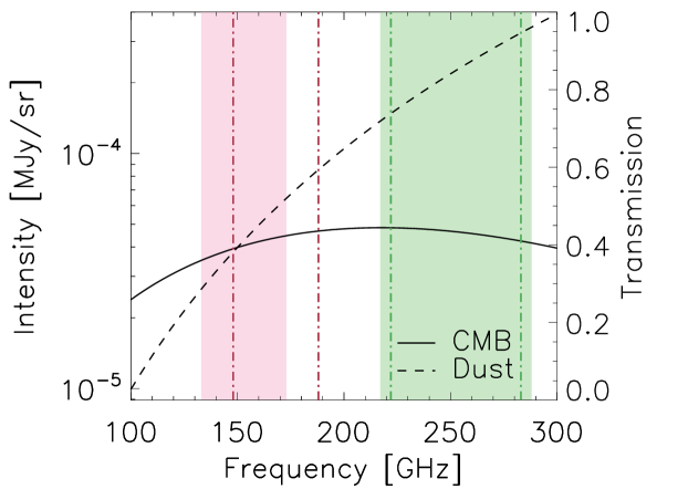
Figure 1: Illustration of the definition of scaling coefficient $\eta$. In this example we have two sky signal components: CMB and polarized Galactic thermal dust emission. There are two top-hat bands centered at 150 and 250 GHz. Left panel: CMB (solid) and Galactic thermal dust (dashed) spectra. For the CMB spectrum, we use the anisotropy spectrum with a 0.1 $\mu K_{\textrm{CMB}}$ signal level, which is the inflationary $B$-mode signal level at $\ell=80$ with a tensor-to-scalar ratio $r=0.1$. The dust spectrum is a 19.6 K blackbody with a 1.59 power law emissivity (Planck Collaboration, 2015b) scaled to a signal level equal to 0.1 $\mu K_{\textrm{CMB}}$ at 150 GHz. The two solid bands are the assumed bands while the two dot-dashed bands are the nominal bands in the simulation. Compared to the assumed band, the nominal 150 GHz band is shifted by 15 GHz with the same band-width. The nominal 250 GHz band has a 10 GHz less band-width compared to the assumed 250 GHz band while having the same band center. Right panel: the CMB and dust intensity integrated over the bands. The CMB and dust data points are offset along the x-axis for clarity. The scaling coefficients are the ratios of the nominal band-integrated signal (plus - CMB, cross - dust) to the assumed band-integrated signal (diamond - CMB, dot - dust). CMB and dust have different scaling coefficients even with the same band mismatch.

In our extended foreground estimation formalism we find the maximum likelihood solution for the foreground spectral parameters $\beta$ and for the scaling coefficients $\eta$. A range of probable scaling coefficients, as obtained from the likelihood function, are mappable to possible combinations of band-centers and band-widths.

The technical implementation is carried out by introducing a new mixing matrix $A$${}_{\textrm{B}}($$\beta,\eta$$)$, which has the same rank as the original mixing matrix $A$, but explicitly includes the scaling coefficients. Each $n_{s}$ by $n_{s}$ block in $A$${}_{\textrm{B}}$ is multiplied by the scaling coefficient for the corresponding frequency channel and sky component. With $A$${}_{\textrm{B}}$ the data model is

$$\boldsymbol{d}=\boldsymbol{A}_{\textrm{B}}(\boldsymbol{\beta},\boldsymbol{\eta})\ \boldsymbol{s}\ +\ \boldsymbol{n}$$ (9)

and the likelihood function is

$$-2\ln\mathcal{L}_{\textrm{B}}(\boldsymbol{s},\boldsymbol{\beta},\boldsymbol{\eta})\ =\ \textrm{const}\ +\ (\boldsymbol{d}-\boldsymbol{A}_{\textrm{B}}\ \boldsymbol{s})^{t}\ \boldsymbol{N}^{-1}\ (\boldsymbol{d}-\boldsymbol{A}_{\textrm{B}}\ \boldsymbol{s}).$$ (10)

When the likelihood reaches maximum we have

$$-2\ln\mathcal{L}_{\textrm{B}}\ =\ \textrm{const}\ -\ (\boldsymbol{A}_{\textrm{B}}^{t}\ \boldsymbol{N}^{-1}\ \boldsymbol{d})^{t}\ (\boldsymbol{A}_{\textrm{B}}^{t}\ \boldsymbol{N}^{-1}\ \boldsymbol{A}_{\textrm{B}})^{-1}\ (\boldsymbol{A}_{\textrm{B}}^{t}\ \boldsymbol{N}^{-1}\ \boldsymbol{d}),$$ (11)

and

$$\boldsymbol{s}\ =\ (\boldsymbol{A}_{\textrm{B}}^{t}\ \boldsymbol{N}^{-1}\ \boldsymbol{A}_{\textrm{B}})^{-1}\ \boldsymbol{A}_{\textrm{B}}^{t}\ \boldsymbol{N}^{-1}\ \boldsymbol{d}.$$ (12)

There exist two degeneracies in the problem. First, the signal level is degenerate with the scaling coefficients. For a particular sky component, simultaneously multiplying all the scaling coefficients by a factor is equivalent to multiplying the sky signal by the same factor. Second, the spectral parameters and the scaling coefficients are degenerate. Tilting the spectrum is equivalent to changing the scaling coefficients by corresponding factors. Figure 2 shows an illustration of this degeneracy. In the example, a mis-estimate of the polarized Galactic thermal dust spectral index by 0.2 has the same $\eta_{\textrm{150,d}}$ and $\eta_{\textrm{250,d}}$ as an 8.5 GHz shift of the band-center at the 150 band toward lower frequency and a 6 GHz reduction of the band-width at the 250 band.

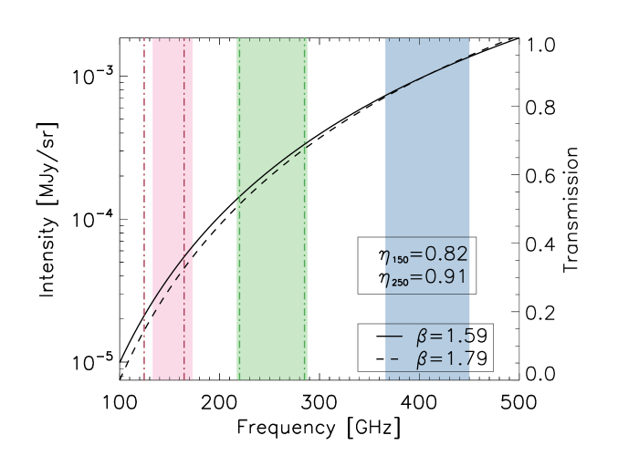
Figure 2: Illustration of degeneracy between the scaling coefficient for polarized Galactic thermal dust $\eta_{\textrm{d}}$ and the dust spectral index $\beta$. We have an assumed dust spectrum (solid) and three assumed frequency bands centered at 150 GHz, 250 GHz and 410 GHz (filled color bands). The dust spectrum has a spectral index of 1.59 and a signal level of 0.1 $\mu K_{\textrm{CMB}}$ at 150 GHz. If the nominal dust spectrum (dashed) has a spectral index of 1.79 and is normalized to the assumed dust spectrum at 410 GHz band, we have $\eta_{\textrm{150,d}}=0.82$ and $\eta_{\textrm{250,d}}=0.91$. If the nominal 150 GHz band is shifted to lower frequency by 8.5 GHz and the nominal 250 GHz band has reduced band-width by 6 GHz compared to the assumed bands, we also have $\eta_{\textrm{150}}=0.82$ and $\eta_{\textrm{250}}=0.91$.

The degeneracies can be broken by setting priors on the scaling coefficients based on the uncertainty of the frequency band measurements. If we assume $\eta_{i}$ is measured with an uncertainty $\sigma_{\eta_{i}}$ around $\bar{\eta_{i}}$, the likelihood function becomes

$$-2\ln\mathcal{L}_{\textrm{B}}(\boldsymbol{\beta},\boldsymbol{\eta})\ =\ \textrm{const}\ -\ (\boldsymbol{A}_{\textrm{B}}^{t}\boldsymbol{N}^{-1}\boldsymbol{d})^{t}\ (\boldsymbol{A}_{\textrm{B}}^{t}\boldsymbol{N}^{-1}\boldsymbol{A}_{\textrm{B}})^{-1}\ (\boldsymbol{A}_{\textrm{B}}^{t}\boldsymbol{N}^{-1}\boldsymbol{d})\ +\ \sum\limits_{i}\frac{(\eta_{i}-\bar{\eta_{i}})^{2}}{\sigma_{\eta_{i}}^{2}},$$ (13)

where the last term represents the priors on the scaling coefficients. We use Eq. 13 to find the best fit spectral parameters and the scaling coefficients. We then recover the sky component signals using the best fit parameters.

2.2.2 Frequency Dependent Polarization Rotation

Frequency dependent polarization rotation mixes the $Q$ and $U$ signals. The amount of rotation within a band depends on the spectral shape of the incoming signals, the characteristic parameters of the instrument, and the frequency band shape.

To incorporate instrumental frequency dependent rotation into foreground estimation, we introduce a new mixing matrix $A$${}_{\textrm{R}}($$\beta,\theta$$)$ which has the same rank as the original mixing matrix $A$. The mixing matrix $A$${}_{\textrm{R}}$ is parameterized by the spectral parameters $\beta$ and a vector $\theta$ of rotation angles for each sky signal component in each frequency band. Compared to $A$, the $2\times 2$ $Q$-$U$ blocks for each sky signal component $s$ at each frequency band $\nu$ in $A$${}_{\textrm{R}}$ are multiplied by rotation matrices with non-zero rotation angles $\theta$_s,ν. Thus each $Q$-$U$ block has non-zero off-diagonal elements and $A$${}_{\textrm{R}}$ is not block diagonal. A requirement on the uncertainty of the rotation angles translates to a requirement on the uncertainty of polarization angle calibration.

With $A$${}_{\textrm{R}}$ the data model is

$$\boldsymbol{d}\ =\ \boldsymbol{A}_{\textrm{R}}(\boldsymbol{\beta},\boldsymbol{\theta})\ \boldsymbol{s}\ +\ \boldsymbol{n},$$ (14)

and the likelihood function is

$$-2\ln\ \mathcal{L}_{\textrm{R}}(\boldsymbol{s},\boldsymbol{\beta},\boldsymbol{\theta})\ =\ \textrm{const}\ +\ (\boldsymbol{d}\ -\ \boldsymbol{A}_{\textrm{R}}\ \boldsymbol{s})^{t}\ \boldsymbol{N}^{-1}\ (\boldsymbol{d}\ -\ \boldsymbol{A}_{\textrm{R}}\ \boldsymbol{s}).$$ (15)

When the likelihood reaches its maximum we have

$$-2\ln\ \mathcal{L}_{\textrm{R}}\ =\ \textrm{const}\ -\ (\boldsymbol{A}_{\textrm{R}}^{t}\ \boldsymbol{N}^{-1}\ \boldsymbol{d})^{t}\ (\boldsymbol{A}_{\textrm{R}}^{t}\ \boldsymbol{N}^{-1}\ \boldsymbol{A}_{\textrm{R}})^{-1}\ (\boldsymbol{A}_{\textrm{R}}^{t}\ \boldsymbol{N}^{-1}\ \boldsymbol{d}),$$ (16)

and

$$\boldsymbol{s}\ =\ (\boldsymbol{A}_{\textrm{R}}^{t}\ \boldsymbol{N}^{-1}\ \boldsymbol{A}_{\textrm{R}})^{-1}\ \boldsymbol{A}_{\textrm{R}}^{t}\ \boldsymbol{N}^{-1}\ \boldsymbol{d}.$$ (17)

There exists a degeneracy between the frequency dependent polarization rotation and the polarization angle of the incoming signal. Changing the band averaged rotation angles of a sky component in all bands by a given amount is equivalent to changing the incoming polarization signal by the same amount. This degeneracy can be broken by setting priors on the rotation angles based on the uncertainty of the polarization angle calibration. If we assume the band averaged rotation angle $\theta_{i}$ is determined within an uncertainty $\sigma_{\theta_{i}}$ around $\bar{\theta_{i}}$ given the knowledge of the instrument and the incoming signals, the likelihood function becomes

$$-2\ln\mathcal{L}_{\textrm{R}}(\boldsymbol{\beta},\boldsymbol{\theta})\ =\ \textrm{const}\ -\ (\boldsymbol{A}_{\textrm{R}}^{t}\boldsymbol{N}^{-1}\boldsymbol{d})^{t}\ (\boldsymbol{A}_{\textrm{R}}^{t}\boldsymbol{N}^{-1}\boldsymbol{A}_{\textrm{R}})^{-1}\ (\boldsymbol{A}_{\textrm{R}}^{t}\boldsymbol{N}^{-1}\boldsymbol{d})\ +\ \sum\limits_{i}\frac{(\theta_{i}-\bar{\theta_{i}})^{2}}{\sigma_{\theta_{i}}^{2}},$$ (18)

where the last term originates from the priors on the rotation angles.

2.2.3 Combining Band Measurement Uncertainty and Frequency Dependent Polarization Rotation

To incorporate both band measurement uncertainty and frequency dependent polarization rotation at the same time we define a new mixing matrix $A$${}_{\textrm{C}}($$\beta$,$\eta$,$\theta$$)$, which has the same rank as the original mixing matrix $A$. Compared to $A$, the mixing matrix $A$${}_{\textrm{C}}$ is parameterized by the spectral parameters $\beta$, the scaling coefficients $\eta$ and the band averaged rotation angles $\theta$. Each $n_{s}$ by $n_{s}$ block in $A$${}_{\textrm{C}}$ is multiplied by the in-band scaling coefficient $\eta_{i}$ for the corresponding signal component and frequency band. The $2\times 2$ $Q$-$U$ block within each $n_{s}$ by $n_{s}$ block is multiplied by a rotation matrix with rotation angle $\theta_{i}$.

With the definition of $A$${}_{\textrm{C}}$ the data model is

$$\boldsymbol{d}\ =\ \boldsymbol{A}_{\textrm{C}}(\boldsymbol{\beta},\boldsymbol{\eta},\boldsymbol{\theta})\ \boldsymbol{s}\ +\ \boldsymbol{n},$$ (19)

and the likelihood function is

$$-2\ln\mathcal{L}_{\textrm{C}}(\boldsymbol{s},\boldsymbol{\beta},\boldsymbol{\eta},\boldsymbol{\theta})\ =\ \textrm{const}\ +\ (\boldsymbol{d}\ -\ \boldsymbol{A}_{\textrm{C}}\ \boldsymbol{s})^{t}\ \boldsymbol{N}^{-1}\ (\boldsymbol{d}\ -\ \boldsymbol{A}_{\textrm{C}}\ \boldsymbol{s}).$$ (20)

When the likelihood reaches its maximum we have

$$-2\ln\mathcal{L}_{\textrm{C}}\ =\ \textrm{const}\ -\ (\boldsymbol{A}_{\textrm{C}}^{t}\ \boldsymbol{N}^{-1}\ \boldsymbol{d})^{t}\ (\boldsymbol{A}_{\textrm{C}}^{t}\ \boldsymbol{N}^{-1}\ \boldsymbol{A}_{\textrm{C}})^{-1}\ (\boldsymbol{A}_{\textrm{C}}^{t}\ \boldsymbol{N}^{-1}\ \boldsymbol{d}),$$ (21)

and

$$\boldsymbol{s}\ =\ (\boldsymbol{A}_{\textrm{C}}^{t}\ \boldsymbol{N}^{-1}\ \boldsymbol{A}_{\textrm{C}})^{-1}\ \boldsymbol{A}_{\textrm{C}}^{t}\ \boldsymbol{N}^{-1}\ \boldsymbol{d}.$$ (22)

Due to the degeneracies mentioned in Sects. 2.2.1 and 2.2.2, to recover the signals accurately we set priors to the scaling coefficients $\eta$ and the band averaged rotation angles $\theta$ based on the uncertainty of the measurements. The likelihood function becomes

$$-2\ln\mathcal{L}_{\textrm{C}}(\boldsymbol{\beta},\boldsymbol{\eta},\boldsymbol{\theta})\ =\ \textrm{const}\ -\ (\boldsymbol{A}_{\textrm{C}}^{t}\ \boldsymbol{N}^{-1}\ \boldsymbol{d})^{t}\ (\boldsymbol{A}_{\textrm{C}}^{t}\ \boldsymbol{N}^{-1}\ \boldsymbol{A}_{\textrm{C}})^{-1}\ (\boldsymbol{A}_{\textrm{C}}^{t}\ \boldsymbol{N}^{-1}\ \boldsymbol{d})\\ +\ \sum\limits_{i}\frac{(\eta_{i}-\bar{\eta_{i}})^{2}}{\sigma_{\eta_{i}}^{2}}\ +\ \sum\limits_{i}\frac{(\theta_{i}-\bar{\theta_{i}})^{2}}{\sigma_{\theta_{i}}^{2}},$$ (23)

where the last two terms come from the priors.

2.3 Error Propagation

Uncertainties in the spectral parameters and instrumental parameters in the mixing matrix propagate to the estimated sky component signals. We estimate the covariance matrix for the parameters using the inverse of the curvature matrix calculated at the maximum likelihood. In the basic case without systematic effects we have

$$\mbox{\boldmath$\tilde{N}$\unboldmath}_{\beta\beta}\ =\ [(\boldsymbol{A},_{\beta_{i}}\boldsymbol{s})^{t}\ \boldsymbol{N}^{-1}\ (\boldsymbol{A},_{\beta_{j}}\boldsymbol{s})-(\boldsymbol{A},_{\beta_{i}\beta_{j}}\boldsymbol{s})^{t}\ \boldsymbol{N}^{-1}\ (\boldsymbol{d}-\boldsymbol{A\ s})-\boldsymbol{M}^{t}\boldsymbol{\hat{N}M}]^{-1}$$ (24)

for the spectral parameters $\beta$, where $\hat{N}$ is the estimated uncertainty matrix of the sky component maps assuming the mixing matrix is perfectly known

$$\boldsymbol{\hat{N}}\ =\ (\boldsymbol{A}^{t}\ \boldsymbol{N}^{-1}\ \boldsymbol{A})^{-1},$$ (25)

and the $M$ matrix is defined as

$$\boldsymbol{M}\ =\ \boldsymbol{A}^{t}\ \boldsymbol{N}^{-1}\ \boldsymbol{A},_{\beta}\boldsymbol{s}-\boldsymbol{A}^{t},_{\beta}\ \boldsymbol{N}^{-1}\ (\boldsymbol{d}-\boldsymbol{A\ s}).$$ (26)

$A,_{\beta}$ and $A,_{\beta\beta}$ are the first and second order derivatives of the mixing matrix with respect to the spectral parameters, estimated at the best fit values of the spectral parameters. The noise matrix of the estimated sky signals is

$$\boldsymbol{\tilde{N}}_{ss}=\boldsymbol{\hat{N}}+(\boldsymbol{\hat{N}M})\ \boldsymbol{\tilde{N}}_{\beta\beta}\ (\boldsymbol{\hat{N}M})^{t}.$$ (27)

When systematic effects are considered, the mixing matrix $A$ in Eq. 24, Eq. 26 and Eq. 27, is changed to the corresponding extended mixing matrix ($A$${}_{\textrm{B}}$, $A$${}_{\textrm{R}}$ or $A$${}_{\textrm{C}}$) and the derivative of the mixing matrix is performed with respect to all corresponding unknown parameters including the spectral parameters $\beta$, the scaling coefficients $\eta$ and the band averaged rotation angles $\theta$.

3 Simulations

We test the extended foreground estimation formalism using simulations. We select a $20^{\circ}\times 20^{\circ}$ sky patch centered on RA = $55^{\circ}$, DEC = $-45^{\circ}$ and include only the CMB and Galactic dust as sky signals. The input CMB angular power spectra are generated with Code for Anisotropies in the Microwave Background (CAMB) described in Lewis et al. (2000) using the Wilkinson Microwave Anisotropy Probe (WMAP) seven-year best-fit cosmological parameters (Komatsu et al., 2011) and a tensor to scalar ratio of $r=0.05$. With a flat-sky approximation (Kaiser, 1992) we generate random Fourier amplitudes in temperature and polarization to match the $C_{\ell}$ power spectra, which are then transformed to CMB maps on the chosen square patch of sky. We adopt the process to generate Galactic dust foreground detailed in Stivoli et al. (2010). The dust intensity and its frequency scaling are given by an $19.6$ K blackbody with a 1.59 power-law emissivity according to the recent Planck measurement (Planck Collaboration, 2015b). The dust polarization fraction is set to 10%. Both the dust frequency scaling and the dust polarization fraction are assumed to be spatially uniform. The large scale polarization angle patterns ($\ell\lesssim 100$) are derived from WMAP dust polarization template (Page et al., 2007). On small angular scales a Gaussian fluctuation power is added using the recipe described in Giardino et al. (2002). Figure 3 shows the $Q$ and $U$ maps of the dust signal and one realization of CMB in the selected sky patch.

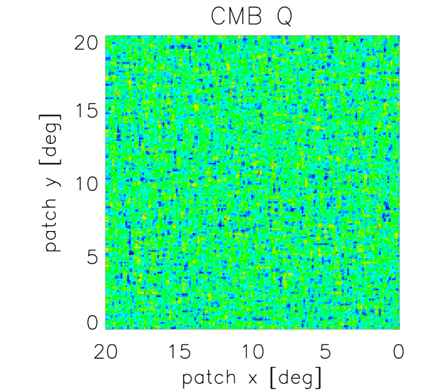
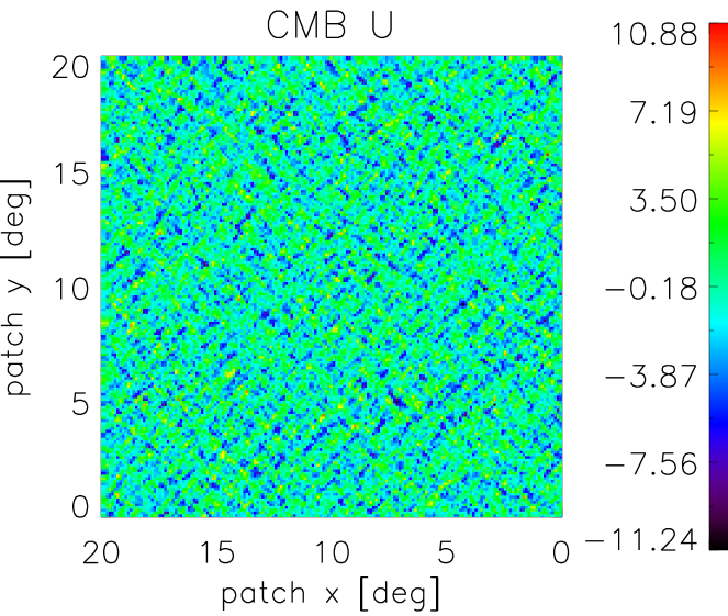
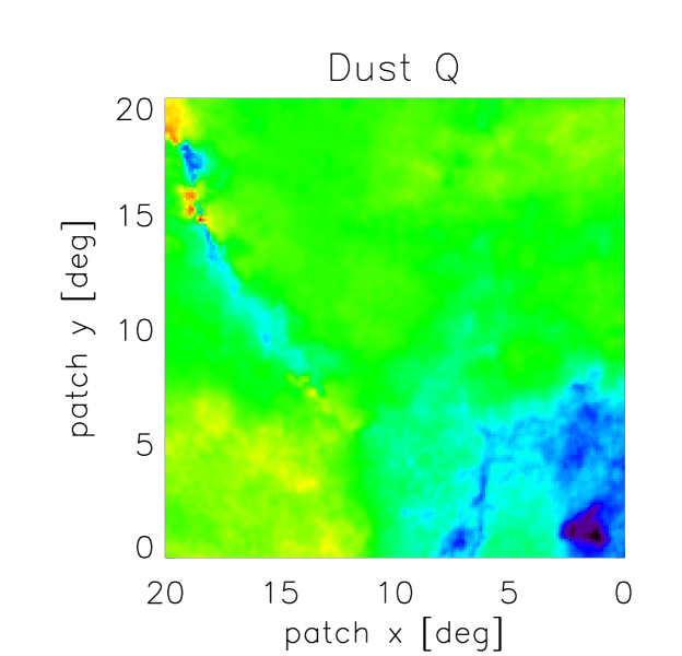
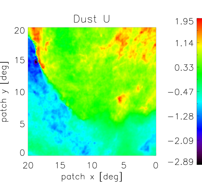
Figure 3: $Q$ (left column) and $U$ (right column) maps of one realization of CMB (top row) and dust (bottom row) at 150 GHz band on the sky patch chosen for simulation. The maps are in units of $\mu K_{\textrm{RJ}}$. The dust signal is simulated using the same procedure as Stivoli et al. (2010). The polarization fraction is assumed to be 10%, while the polarization angle is derived by the WMAP observations on large scales ($\ell\lesssim 100$), and Gaussian power at small scales.

The observations are simulated in three top-hat bands centered at 150 GHz, 250 GHz and 410 GHz. The frequency ranges for the three bands and their noise levels per $6.87^{\prime}\times 6.87^{\prime}$ square pixel in the $Q$ and $U$ maps are listed in Table 1. The noise is assumed to be uniform and white across the patch. The noise realization is added to the signal in the map domain in all simulations.

Top-hat band	Frequency range [GHz]	Pixel Noise [$\mu K_{\textrm{RJ}}$]
150 GHz	[133, 173]	0.8
250 GHz	[217, 288]	1.0
410 GHz	[366, 450]	1.4

Table 1: Top-hat bands and the corresponding noise per $6.87^{\prime}\times 6.87^{\prime}$ pixel in the $Q$ and $U$ maps used in the simulation.

In the simulation we include a continuously rotating achromatic half-wave plate (AHWP) which induces a frequency dependent polarization rotation. The AHWP is composed of a stack of five single sapphire half-wave plates with an average thickness of 1.65 mm. The relative orientation angles between the optical axis of the plates and the first plate in the stack are 0^∘, 28^∘, 94^∘, 28^∘, 0^∘. The ordinary and extraordinary refractive indices of sapphire at cryogenic temperature are used to calculate the instrumental polarization rotation angles, i.e., $n_{o}\ =\ 3.047$ and $n_{e}\ =\ 3.361$ (Afsar & Chi, 1991; Loewenstein et al., 1973). We model the AHWP using Mueller matrices formalism described in Matsumura et al. (2009). Given the frequency bands, the input dust spectrum and the AHWP parameters, the rotation angles are 115.66^∘, 103.64^∘, 110.76^∘ for CMB and 115.02^∘, 103.68^∘, 112.88^∘ for dust at 150, 250, 410 GHz bands, respectively . Figure 4 shows the observed $Q$ and $U$ maps at 150 GHz band. They include both CMB, and dust, rotation induced by the AHWP, and instrumental noise. The parameters of the AHWP and the noise levels were chosen to be close to those designed for the EBEX balloon-borne instrument.

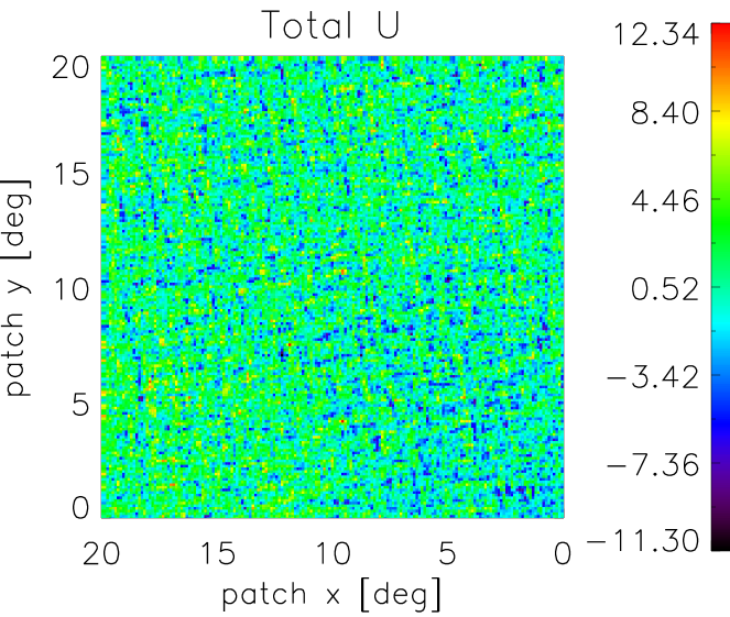
Figure 4: $Q$ (left) and $U$ (right) maps of observation at 150 GHz band with AHWP rotation effect and instrumental noise included. This is one realization of the CMB and instrumental noise. The maps are in units of $\mu K_{\textrm{RJ}}$.

The $EE$ and $BB$ power spectra are calculated simultaneously using a flat-sky approximation (Kaiser, 1992). For each set of input parameters, the simulation is run 100 times with different CMB and noise realizations while the dust signal is kept the same. The result shown for any given $\ell$ bin is the mean of the 100 simulations and the error bar is the standard deviation. Specifically, the error bars of the input CMB spectrum are the cosmic variances while the error bars of the output CMB spectrum also include uncertainties from the instrumental noise and the propagation of the parameter uncertainties. We also calculate residual power spectra. For each of the 100 simulations the residual spectrum is the difference between the estimated CMB spectrum, after estimation of the foreground, and the input spectrum. We plot the mean and the standard deviations of the 100 simulations. We consider the estimated CMB $B$-mode power spectrum ‘biased’ using two criteria such that each provides somewhat different information: (1) when the estimated CMB $B$-mode signal power is more than twice the cosmic variance away from the input in any $\ell$ bin, and (2) when the residual power spectrum is more than one sigma away from zero. The first criterion quantifies bias relative to irreducible cosmic variance and is particularly useful for noiseless simulations. The second is more relevant when instrument noise is included and is less stringent than the first.

For the simulations the data model in the basic formalism

$$\boldsymbol{d\ =\ A\ s\ +\ n},$$ (28)

becomes

$$\scalebox{0.78}{\mbox{$\displaystyle\left(\begin{array}[]{c}I_{150}\\ Q_{150}\\ U_{150}\\ I_{250}\\ Q_{250}\\ U_{250}\\ I_{410}\\ Q_{410}\\ U_{410}\end{array}\right)=\left(\begin{array}[]{cccccc}A_{150,{\textrm{c}}}&0&0&A_{150,{\textrm{d}}}(\beta)&0&0\\ 0&A_{150,{\textrm{c}}}&0&0&A_{150,{\textrm{d}}}(\beta)&0\\ 0&0&A_{150,{\textrm{c}}}&0&0&A_{150,{\textrm{d}}}(\beta)\\ A_{250,{\textrm{c}}}&0&0&A_{250,{\textrm{d}}}(\beta)&0&0\\ 0&A_{250,{\textrm{c}}}&0&0&A_{250,{\textrm{d}}}(\beta)&0\\ 0&0&A_{250,{\textrm{c}}}&0&0&A_{250,{\textrm{d}}}(\beta)\\ A_{410,{\textrm{c}}}&0&0&A_{410,{\textrm{d}}}(\beta)&0&0\\ 0&A_{410,{\textrm{c}}}&0&0&A_{410,{\textrm{d}}}(\beta)&0\\ 0&0&A_{410,{\textrm{c}}}&0&0&A_{410,{\textrm{d}}}(\beta)\end{array}\right)\left(\begin{array}[]{c}I_{CMB}\\ Q_{CMB}\\ U_{CMB}\\ I_{dust}\\ Q_{dust}\\ U_{dust}\end{array}\right)+\left(\begin{array}[]{c}n_{I_{150}}\\ n_{Q_{150}}\\ n_{U_{150}}\\ n_{I_{250}}\\ n_{Q_{250}}\\ n_{U_{250}}\\ n_{I_{410}}\\ n_{Q_{410}}\\ n_{U_{410}}\end{array}\right)$}}.$$ (29)

Here $I$, $Q$ and $U$ are the polarization stokes parameters. The subscripts denote frequency bands and components. The elements in the mixing matrix related to CMB are known since we know the CMB spectrum. For any given frequency $\nu$, the element in the mixing matrix related to dust is

$$A_{\nu,{\textrm{d}}}(\beta)\ =\ \Big{(}\frac{\nu}{\nu_{0}}\Big{)}^{\beta}B_{\nu}(T_{\textrm{d}},\nu),$$ (30)

where $\nu_{0}$ is a reference frequency typically set to the center of the highest frequency channel of the experiment, $B_{\nu}$ is the blackbody spectrum, $T_{\textrm{d}}$ is the dust temperature (which is assumed to be known) and $\beta$ is the spectral index of dust which is the sole unknown parameter in this case.

When band measurement uncertainties are included, the mixing matrix becomes

$$\boldsymbol{A}_{\textrm{B}}=\left(\scalebox{0.78}{\mbox{$\displaystyle\begin{array}[]{cccccc}A_{150,{\textrm{c}}}\eta_{150,{\textrm{c}}}&0&0&A_{150,{\textrm{d}}}(\beta)\eta_{150,{\textrm{d}}}&0&0\\ 0&A_{150,{\textrm{c}}}\eta_{150,{\textrm{c}}}&0&0&A_{150,{\textrm{d}}}(\beta)\eta_{150,{\textrm{d}}}&0\\ 0&0&A_{150,{\textrm{c}}}\eta_{150,{\textrm{c}}}&0&0&A_{150,{\textrm{d}}}(\beta)\eta_{150,{\textrm{d}}}\\ A_{250,{\textrm{c}}}\eta_{250,{\textrm{c}}}&0&0&A_{250,{\textrm{d}}}(\beta)\eta_{250,{\textrm{d}}}&0&0\\ 0&A_{250,{\textrm{c}}}\eta_{250,{\textrm{c}}}&0&0&A_{250,{\textrm{d}}}(\beta)\eta_{250,{\textrm{d}}}&0\\ 0&0&A_{250,{\textrm{c}}}\eta_{250,{\textrm{c}}}&0&0&A_{250,{\textrm{d}}}(\beta)\eta_{250,{\textrm{d}}}\\ A_{410,{\textrm{c}}}\eta_{410,{\textrm{c}}}&0&0&A_{410,{\textrm{d}}}(\beta)\eta_{410,{\textrm{d}}}&0&0\\ 0&A_{410,{\textrm{c}}}\eta_{410,{\textrm{c}}}&0&0&A_{410,{\textrm{d}}}(\beta)\eta_{410,{\textrm{d}}}&0\\ 0&0&A_{410,{\textrm{c}}}\eta_{410,{\textrm{c}}}&0&0&A_{410,{\textrm{d}}}(\beta)\eta_{410,{\textrm{d}}}\\ \end{array}$}}\right).$$ (31)

There are seven unknown parameters in $A$${}_{\textrm{B}}$: the dust spectral index and six scaling coefficients.

When the frequency dependent polarization rotation is included, the mixing matrix becomes

$$\boldsymbol{A}_{\textrm{R}}=\left(\begin{array}[]{cc}\boldsymbol{A}_{\textrm{$R_{1}50,\textrm{c}$}}&\boldsymbol{A}_{\textrm{$R_{150,d}$}}\\ \boldsymbol{A}_{\textrm{$R_{250,c}$}}&\boldsymbol{A}_{\textrm{$R_{250,d}$}}\\ \boldsymbol{A}_{\textrm{$R_{410,c}$}}&\boldsymbol{A}_{\textrm{$R_{410,d}$}}\\ \end{array}\right),$$ (32)

with the blocks $A$${}_{\textrm{$R_{\nu,s}$}}$ for CMB and dust at frequency band $\nu$ being

$$\boldsymbol{A}_{\textrm{$R_{\nu,c}$}}=\left(\begin{array}[]{ccc}A_{\nu,{\textrm{c}}}&0&0\\ 0&A_{\nu,{\textrm{c}}}\cos\theta_{\nu,{\textrm{c}}}&-A_{\nu,{\textrm{c}}}\sin\theta_{\nu,{\textrm{c}}}\\ 0&A_{\nu,{\textrm{c}}}\sin\theta_{\nu,{\textrm{c}}}&A_{\nu,{\textrm{c}}}\cos\theta_{\nu,{\textrm{c}}}\\ \end{array}\right),$$

$$\boldsymbol{A}_{\textrm{$R_{\nu,d}$}}=\left(\begin{array}[]{ccc}A_{\nu,{\textrm{d}}}(\beta)&0&0\\ 0&A_{\nu,{\textrm{d}}}(\beta)\cos\theta_{\nu,{\textrm{d}}}(\beta)&-A_{\nu,{\textrm{d}}}(\beta)\sin\theta_{\nu,{\textrm{d}}}(\beta)\\ 0&A_{\nu,{\textrm{d}}}(\beta)\sin\theta_{\nu,{\textrm{d}}}(\beta)&A_{\nu,{\textrm{d}}}(\beta)\cos\theta_{\nu,{\textrm{d}}}(\beta)\\ \end{array}\right),$$

where the subscript $\nu$ runs over 150, 250, and 410 GHz. There are seven unknown parameters in $A$${}_{\textrm{R}}$: the dust spectral index and six rotation angles.

When both the band measurement uncertainty and the frequency dependent rotation effect of the AHWP are considered, the mixing matrix becomes

$$\boldsymbol{A}_{\textrm{C}}=\left(\begin{array}[]{cc}\boldsymbol{A}_{\textrm{$C_{150,c}$}}&\boldsymbol{A}_{\textrm{$C_{150,d}$}}\\ \boldsymbol{A}_{\textrm{$C_{250,c}$}}&\boldsymbol{A}_{\textrm{$C_{250,d}$}}\\ \boldsymbol{A}_{\textrm{$C_{410,c}$}}&\boldsymbol{A}_{\textrm{$C_{410,d}$}}\\ \end{array}\right),$$ (33)

with the blocks $A$${}_{\textrm{C}_{\nu,s}}$ for CMB and dust at frequency channel $\nu$ being

$$\boldsymbol{A}_{\textrm{C}_{\nu,\textrm{c}}}=\left(\begin{array}[]{ccc}\eta_{\nu,{\textrm{c}}}A_{\nu,{\textrm{c}}}&0&0\\ 0&\eta_{\nu,{\textrm{c}}}A_{\nu,{\textrm{c}}}\cos\theta_{\nu,{\textrm{c}}}&-\eta_{\nu,{\textrm{c}}}A_{\nu,{\textrm{c}}}\sin\theta_{\nu,{\textrm{c}}}\\ 0&\eta_{\nu,{\textrm{c}}}A_{\nu,{\textrm{c}}}\sin\theta_{\nu,{\textrm{c}}}&\eta_{\nu,{\textrm{c}}}A_{\nu,{\textrm{c}}}\cos\theta_{\nu,{\textrm{c}}}\\ \end{array}\right),$$

$$\boldsymbol{A}_{\textrm{C}_{\nu,\textrm{d}}}=\left(\begin{array}[]{ccc}\eta_{\nu,{\textrm{d}}}A_{\nu,{\textrm{d}}}(\beta)&0&0\\ 0&\eta_{\nu,{\textrm{d}}}A_{\nu,{\textrm{d}}}(\beta)\cos\theta_{\nu,{\textrm{d}}}(\beta)&-\eta_{\nu,{\textrm{d}}}A_{\nu,{\textrm{d}}}(\beta)\sin\theta_{\nu,{\textrm{d}}}(\beta)\\ 0&\eta_{\nu,{\textrm{d}}}A_{\nu,{\textrm{d}}}(\beta)\sin\theta_{\nu,{\textrm{d}}}(\beta)&\eta_{\nu,{\textrm{d}}}A_{\nu,{\textrm{d}}}(\beta)\cos\theta_{\nu,{\textrm{d}}}(\beta)\\ \end{array}\right),$$

where the subscript $\nu$ runs over 150, 250 and 410 GHz. There are a total of 13 unknown parameters in $A$${}_{\textrm{C}}$: the dust spectral index, six scaling coefficients and six band averaged rotation angles. Note that $A$${}_{\textrm{C}}$ reduce to $A$${}_{\textrm{B}}$ in the case of $\theta_{\nu,{\textrm{c}}}=\theta_{\nu,{\textrm{d}}}=0$ and reduce to $A$${}_{\textrm{R}}$ in the case of $\eta_{\nu,{\textrm{c}}}=\eta_{\nu,{\textrm{d}}}=1$. In our simulations, when setting priors to parameters, we assume a Gaussian prior with quoted FWHM values.

4 Results

4.1 Consistency Check

In the absence of band measurement and polarization angle calibration uncertainties the extended formalism reproduces the input spectra with no bias; this is shown in Fig. 5. For this simulation we included the systematic effects but they were assumed to be perfectly known. In all the power spectra plots shown in the rest of this section, the data points of the estimated CMB $B$-mode power spectrum are plotted offset along the x-axis for clarity. We also plot the theoretical underlying CMB $B$-mode power spectrum with $r=0.05$.

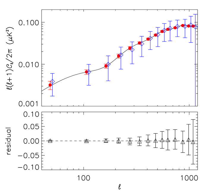
Figure 5: Demonstration of the validity of the extended formalism assuming perfect knowledge of the scaling coefficients and the rotation angles. The dust spectral index is the only parameter estimated here. Top: $B$-mode angular power spectra of the input CMB (red dot, error bars include only cosmic variance) and the estimated CMB (blue diamond). No bias is introduced in the final estimated CMB $B$-mode signal compared to the input. The solid black line is the theoretical CMB $B$-mode power spectrum assuming $r=0.05$. Bottom: residual angular power spectrum between the estimated CMB $B$-mode signal and the input. The residual (black triangle) is consistent with zero (dashed line) in all $\ell$ bins.

Next we assess the intrinsic bias in the estimated CMB signal induced by the formalism in the absence of instrumental noise. Due to the degeneracies discussed in Sec. 2.2, here we consider the systematic effects in only one band at a time while assuming the other two bands are perfectly known. All the parameters in the mixing matrix are estimated without any priors. We test the formalism including band measurement uncertainty only, frequency dependent polarization rotation only, or both systematic effects. The estimated CMB $B$-mode signal is not biased in all of the cases. Figure 6 shows an example when both band measurement uncertainty and frequency dependent polarization rotation are considered at 150 GHz band. When the 150 GHz band-center or band-width is mis-estimated by 15 GHz, the estimated scaling coefficients and CMB $B$-mode signal are without any bias. Similarly, the formalism does not bias the CMB $B$-mode signal with a mis-estimation of 15 GHz of the band-center or band-width at 250 or 410 GHz band. We also see similar results when only one of the systematic effects is considered.

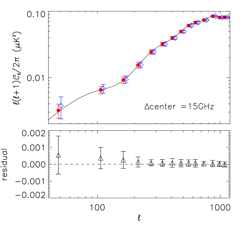
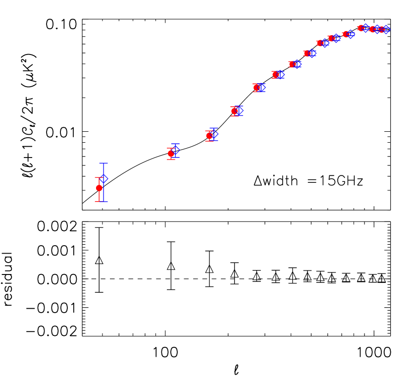
Figure 6: Simulation results where the band measurement uncertainty and frequency dependent polarization rotation are included only for 150 GHz band in the absence of instrumental noise. The 250 GHz and 410 GHz bands are assumed to be perfectly known. The band-center (left) or the band-width (right) of the 150 GHz band is mis-estimated by 15 GHz. In both cases the estimated the CMB $B$-mode signal (blue diamond) is not biased compared to the input signal (red dot), and the residual (black triangle) is consistent with zero.

4.2 Band Measurement Uncertainty

When estimating the CMB $B$-mode signal in the presence of band measurement uncertainty and instrumental noise, all the band averaged rotation angles are assumed to be perfectly known.

First we address the cases where there are uncertainties in only one of the bands. As discussed in Sec. 2.2.1 we observe a degeneracy between the dust spectral index and the dust scaling coefficient. When noise is present in the observation, changing the tilt of the dust spectrum or the scaling of the dust signal in one band give similar likelihood. The degeneracy causes bias in the recovered CMB power spectrum, particularly in the low-$\ell$ bins where the dust signal is high and the inflationary $B$-mode signal resides. Figure 7 shows the 2-D likelihood plot between the dust spectral index and the dust scaling coefficient and the estimated CMB $B$-mode power spectrum when there are uncertainties at 150 GHz band only. The points along the bright diagonal feature in the likelihood plot have similar likelihood. When the parameters are mis-estimated, the estimated $B$-mode signal is biased by at low $\ell$.

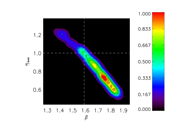
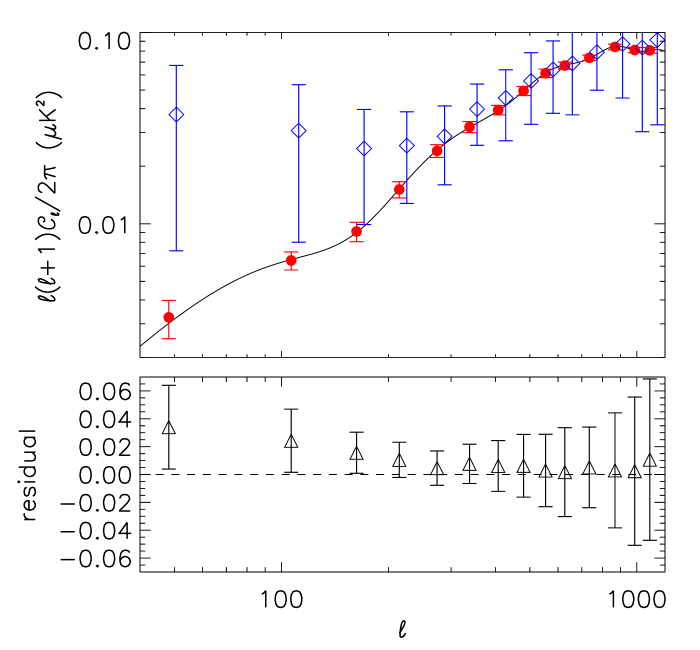
Figure 7: Degeneracy between spectral index and dust scaling coefficient exists and it causes bias in the estimated CMB $B$-mode power spectrum at low $\ell$. The scaling coefficients at 250 GHz and 410 GHz bands are assumed to be perfectly known. Only the two coefficients at 150 GHz are being optimized. Left: 2-D likelihood plot between the dust spectral index $\beta$ and the dust scaling coefficient $\eta_{\textrm{d}}$ at 150 GHz. The bright diagonal feature in the 2-D parameter space shows that points along the strip give similar likelihood and thus are degenerate. The two white dashed lines are the input values of the two parameters. The input values, although on the diagonal feature, is not the point with the highest likelihood in this simulation. Right: Power spectrum (top) and residual power spectrum (bottom) of the CMB $B$-mode. The estimated CMB signal (blue diamond) is biased compared to the input (red dot) and the residual (black triangle) is biased.

Setting priors on the scaling coefficients according to the band measurement uncertainty limits the parameter space in which the best fit values are searched for. In this study the priors are centered on the input value which is one. In the case where the uncertainty of only the 150 GHz band is considered, with 15% Gaussian priors on the scaling coefficients for both CMB and dust the estimated CMB $B$-mode signal is not biased, as shown in Fig. 8.

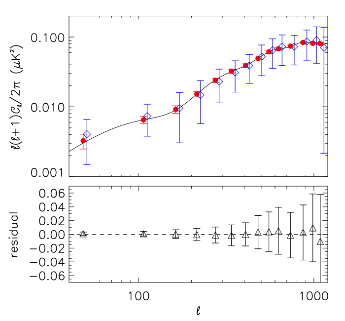
Figure 8: Simulated results with 15% priors on scaling coefficients at 150 GHz band. The coefficients at 250 GHz and 410 GHz bands are assumed to be perfectly known. The estimated CMB signal (blue diamond) agrees with the input (red dot) and the residual (black triangle) is consistent with zero.

When uncertainties of all three bands are included the degeneracy between the scaling coefficients and the sky signal level requires priors on all scaling coefficients. Figure 9 shows two cases where 5% or 10% Gaussian priors are set on all scaling coefficients. When all scaling coefficients have 5% Gaussian priors the $B$-mode signal is estimated accurately. When the priors are relaxed to 10%, the estimated signal in the lowest $\ell$ bin is 2.5 times the cosmic variance away from the input value. The bias comes from the degeneracy between the dust scaling coefficients and the dust spectral index and therefore the bias is strongest at the $\ell$ range in which dust is most intense. If we factor in the effect of the instrumental noise the residual power spectrum is consistent with zero in all $\ell$ bins.

Figure 9: Simulation results where band measurement uncertainties of all three frequency bands are included. 5% (left) or 10% (right) Gaussian priors are set on all scaling coefficients around the input value. When the priors are 5% the estimated CMB $B$-mode signal (blue diamond) agrees with the input CMB signal (red dot). When the priors are relaxed to 10%, the estimated $B$-mode signal at the lowest-$\ell$ bin is 2.5 times the cosmic variance away from the input value. With the effect of instrumental noise, the residual power spectrum (black triangle) is consistent with zero.

Specific priors on the scaling coefficients is analogous to known measurement uncertainties. Table 2 gives the mapping between prior interval on the scaling coefficients and uncertainties in band-center and band-width for the three top-hat bands used in the simulations. The values for band-center uncertainty are calculated assuming the band-width has no uncertainty and vice versa.

	Band mismatch	150 GHz	250 GHz	410 GHz
5% $\eta_{\textrm{d}}$ mismatch	center (GHz)	4.5	7.5	12.0
	width (GHz)	2.0	3.5	4.0
10% $\eta_{\textrm{d}}$ mismatch	center (GHz)	9.5	15.0	25.0
	width (GHz)	4.0	7.0	8.5

Table 2: The band-center and band-width mismatches corresponding to a 5% or 10% $\eta_{\textrm{d}}$ mismatch for the three top-hat bands at 150, 250 and 410 GHz. When calculating the values for band-center, the band-widths are assumed to be perfectly known and vice versa.

In practice, however, both band-center and band-width have uncertainty simultaneously. As an example, in Fig. 10 we show the contour of the scaling coefficient deviation in the 2-D parameter space of band-center and band-width for Galactic dust at 250 GHz band. Similar Figures are obtained for the CMB and other frequency bands as well. Using such Figures, which are easily calculable given any band parameters, one can map band measurement uncertainty to scaling coefficient priors.

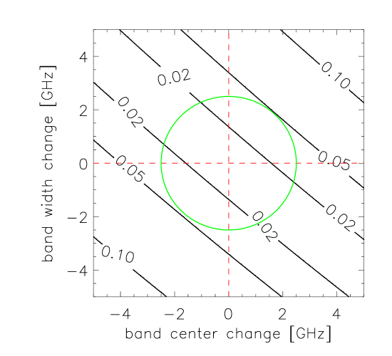
Figure 10: Contours showing percent scaling coefficient deviations from the nominal value of unity translated to band-center and band-width shifts from their nominal value for the 250 GHz band for Galactic dust. The green circle shows the constraint imposed on the scaling coefficient with 2.5 GHz uncertainty for both band-center and band-width. The circle lies entirely within the 5% contour of scaling coefficient deviation implying that 2.5 GHz band measurement uncertainty in this band is equivalent to a 5% prior on $\eta_{\textrm{d}}$.

4.3 Frequency Dependent Polarization Rotation

When assessing only the frequency dependent polarization rotation in the presence of instrumental noise, all the scaling coefficients are assumed to be perfectly known. We first consider the uncertainty of the band averaged rotation angles in only one band while assuming the rotation angles in the other two bands are perfectly known. Since there is no degeneracy between the incoming polarization angle and the AHWP rotation angles in this case, we can estimate the CMB $B$-mode signal accurately without priors on the rotation angles. Figure 11 shows the result where the uncertainty of the polarization angle calibration in only 150 GHz band is considered. We get similar results for 250 GHz and 410 GHz band.

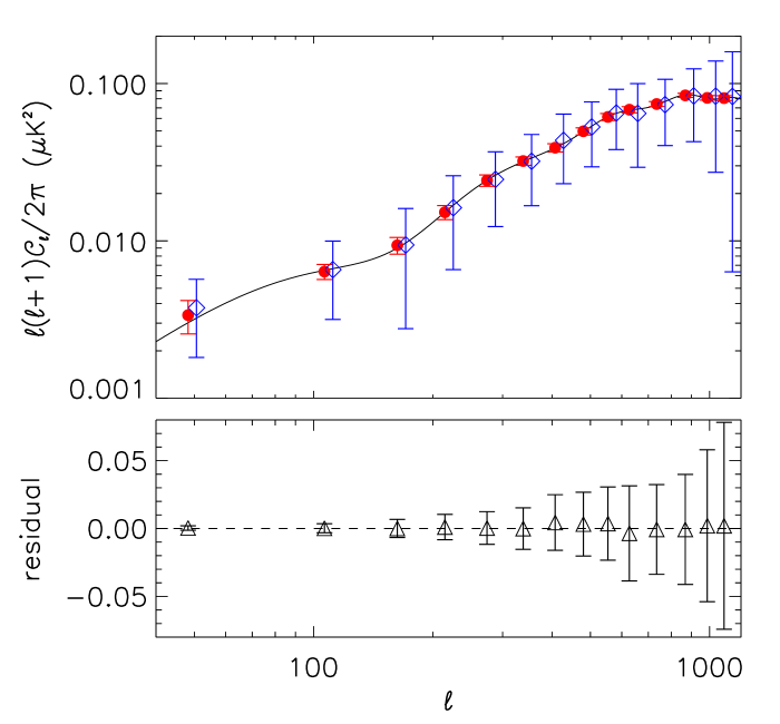
Figure 11: Simulation results where band averaged polarization rotation angles for only 150 GHz band are optimized. No prior constraints are set on the rotation angles at 150 GHz. All angles at 250 GHz and 410 GHz bands are assumed to be perfectly known. The estimated CMB $B$-mode signal (blue diamond) agrees with the input signal (red dot).

When uncertainties of polarization angle calibration in all three bands are included, the degeneracy between the frequency dependent polarization rotation and the polarization angle of the incoming signal requires priors on the band-averaged rotation angles. Here we center the priors on the input value. Figure 12 shows that with 4^∘ Gaussian priors on all band-averaged rotation angles, the final estimated CMB $B$-mode signal is not biased. When the priors are relaxed to 10^∘ the estimated CMB $B$-mode signal is more than twice the cosmic variance away from the input in a few bins at $\ell>300$. Less stringent priors on the band averaged rotation angles result in a bigger mis-estimate of the polarization angle of the incoming signal. This mis-estimate induces leakage from CMB $E$-mode signal to $B$-mode signal which has a bigger effect at high $\ell$. When other noise sources are included the residual power spectrum is consistent with zero in both cases.

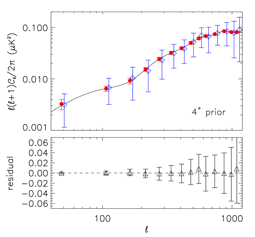
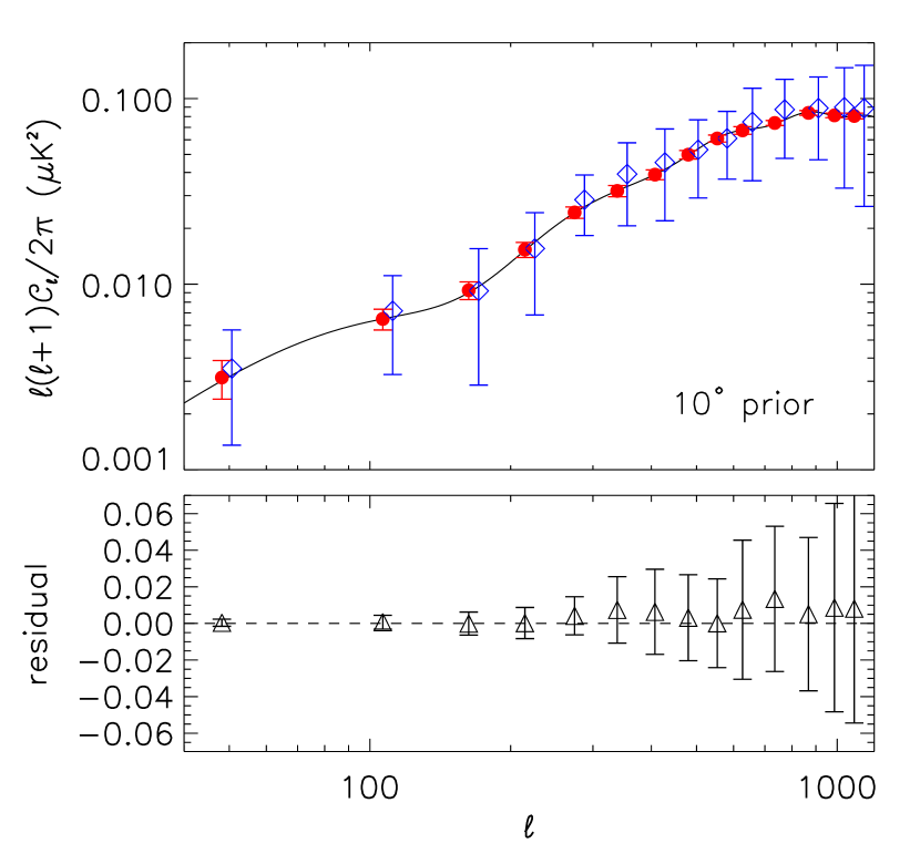
Figure 12: Simulation results where the uncertainties of polarization angle calibration for all three bands are included. Left: 4^∘ Gaussian priors on all rotation angles. Right: 10^∘ Gaussian priors on all rotation angles. When the priors are 4^∘ the estimated CMB $B$-mode signal (blue diamond) agrees with the input signal (red dot). When the priors are 10^∘, the estimated CMB $B$-mode is more than twice the cosmic variance away from the input CMB in a few bins at $\ell>300$ due to the mixing of $E$-mode signal into $B$-mode signal. When the instrumental noise is considered, the residual power spectrum (black triangle) is consistent with zero.

4.4 Combining Band Measurement Uncertainty and Frequency Dependent Polarization Rotation

When both systematic effects are included in the presence of instrumental noise, the formalism estimates the scaling coefficients and the band averaged polarization rotation angles simultaneously. We first assess the bias in the estimated CMB $B$-mode signal including the systematic effects at only one of the bands while assuming the other two bands are perfectly known. In Fig. 13 we show the results where there are systematic effects at 150 GHz only. The estimated CMB $B$-mode signal is not biased with 15% Gaussian priors on the scaling coefficients for CMB and dust and no priors on band averaged rotation angles. We get similar results when there are systematic effects at 250 or 410 GHz band only.

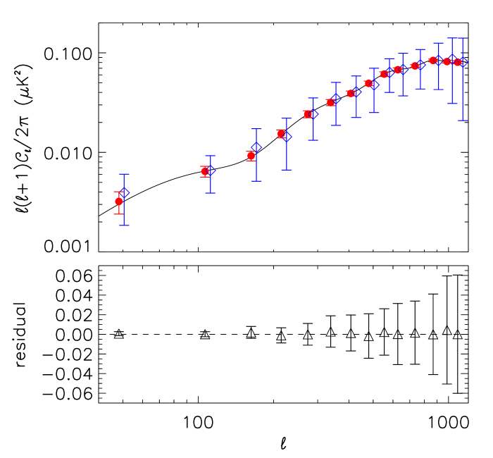
Figure 13: Simulation results where both the band measurement uncertainty and frequency dependent polarization rotation are included for the 150 GHz band in the presence of instrumental noise. There are 15% Gaussian priors on the scaling coefficients and no prior on the band-averaged rotation angles. The parameters for the 250 GHz and 410 GHz bands are assumed to be perfectly known. There is no bias in the estimated CMB $B$-mode signal (blue diamond) compared to the input signal (red dot) and the residual (black triangle) is consistent with zero.

When the systematic effects are considered for all three bands, priors are needed for all parameters due to the degeneracies. Figure 14 shows that with 5% Gaussian prior on scaling coefficients and 4^∘ Gaussian priors on band averaged rotation angles we can estimate CMB $B$-mode signal without any bias.

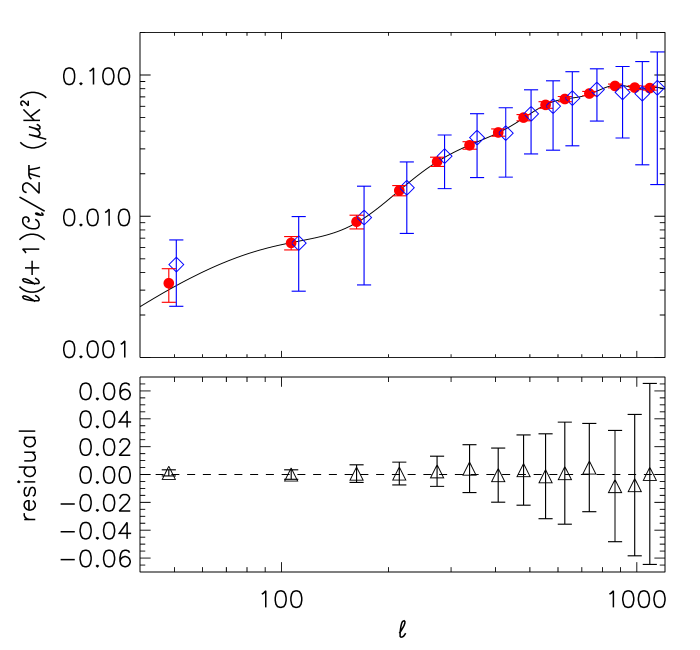
Figure 14: Results of simulation with 5% Gaussian priors on scaling coefficients and 4^∘ Gaussian priors on band averaged rotation angles in the presence of instrumental noise. The estimated CMB signal (blue diamond) is not biased compared to the input (red dot) and the residual (black triangle) is consistent with zero.

4.5 Foreground Estimation with Measured EBEX Bands

As a practical example, we estimate foreground using the measured EBEX bands and their uncertainties, which are shown in Fig. 15 (Zilic, 2014).

Figure 15: Measured EBEX 150 GHz, 250 GHz and 410 GHz bands. The measurements and data analysis to derive these bands are presented in Zilic (2014).

We carry out simulations of the band measurement. Each realization is a simulated measurement of the band given the measured frequency bin errors. For each realization we compute the scaling coefficients compared to the measured band, which are taken to be the nominal values of the measurement, and band averaged rotation angles for CMB and Galactic dust. The standard deviation from the simulated results, listed in Table 3, are considered as the priors on the corresponding parameters.

Priors	150 GHz band	250 GHz band	410 GHz band
$\eta_{CMB}$	5%	4%	5%
$\eta_{dust}$	5%	3%	4%
$\theta_{CMB}$	0.2∘	0.02∘	0.2∘
$\theta_{dust}$	0.2∘	0.02∘	0.2∘

Table 3: Uncertainties of the in-band scaling coefficients $\eta$ and band averaged rotation angles $\theta$ for the three EBEX bands. These values are the standard deviation of the parameters calculated from 500 Monte-Carlo simulations.

Figure 16 shows the power spectra of the simulation with the priors listed in Table 3. We find that with $r=0.05$ an expreimtn like EBEX can estimate the B-mode spectrum without bias at a level comparible to either cosmic variance or instrumental noise.

Figure 16: Simulation results where both systematic effects in all three bands are included. All parameters have priors based on Monte-Carlo simulations using the three EBEX bands, which are listed in Table 3. The estimated CMB $B$-mode signal (blue diamond) agree with the input signal (red dot) without any bias and the residual (black diamond) is consistent with zero.

5 Summary

Recent observations suggest that Galactic dust is a significant contaminating source in all regions of the sky for CMB polarimeters targeting the inflationary $B$-mode signal. The Galactic dust signal needs to be removed and robust foreground estimation is essential. We presented a general maximum likelihood foreground estimation formalism in the presence of two systematic effects: band measurement uncertainty and frequency dependent polarization rotation. The formalism fits the systematic effects simultaneously with the dust spectral index which allows for imperfect knowledge of the instrumental parameters.

We found several degeneracies: 1) between the dust spectral index and the dust scaling coefficients, 2) between the scaling coefficients and the signal levels, and 3) between the frequency dependent polarization rotation and the signal polarization angles. Due to the degeneracies, priors on the parameters are needed in order estimate the CMB $B$-mode signal accurately. We quantified the degeneracies and showed, as an example, that a sub-orbital experiment like EBEX should not be limited in estimating and subtracting Galactic dust if it has 10% polarization fraction, if the tensor to scalar ratio $r=0.05$, and with band measurement and polarization angle calibration uncertainty of 5% and 4^∘, respectively. Such an experiment may not be limited with even higher polarization fractions or lower $r$ values. A detailed calculation is necessary for other concrete cases.

Band measurement uncertainty is a common systematic effect for all CMB instruments. Frequency dependent polarization rotation by elements in the focal plane is not unique to the use of an achromatic half-wave plate either. Sinuous antenna detectors also have frequency dependent polarization rotation (O’Brient et al., 2008). Therefore, the foreground estimation formalism developed in this paper has general applicability.

References

- Afsar & Chi (1991) Afsar, M. N., & Chi, H. 1991, in Society of Photo-Optical Instrumentation Engineers (SPIE) Conference Series, 16th International Conference on Infrared and Millimeter Waves, iSBN 0-8194-0707-0, M. R. Siegrist, M. Q. Tran and T. M. Tran, Lausanne, Switzerland, Aug 26-30, 1991
- Arnold et al. (2010) Arnold, K., et al. 2010, in Society of Photo-Optical Instrumentation Engineers (SPIE) Conference Series, Vol. 7741, Society of Photo-Optical Instrumentation Engineers (SPIE) Conference Series
- Bao et al. (2012) Bao, C., et al. 2012, ApJ, 747, 97
- BICEP2/Keck and Planck Collaborations (2015) BICEP2/Keck and Planck Collaborations. 2015, Physical Review Letters, 114, 101301
- Church et al. (2003) Church, S., Knox, L., & White, M. 2003, ApJ, 582, L63
- Errard & Stompor (2012) Errard, J., & Stompor, R. 2012, Phys. Rev. D, 85, 083006
- Fraisse et al. (2013) Fraisse, A. A., et al. 2013, JCAP, 4, 47
- Giardino et al. (2002) Giardino, G., Banday, A. J., Górski, K. M., Bennett, K., Jonas, J. L., & Tauber, J. 2002, A&A, 387, 82
- Gold et al. (2009) Gold, B., et al. 2009, ApJS, 180, 265
- Kaiser (1992) Kaiser, N. 1992, ApJ, 388, 272
- Kamionkowski et al. (1997) Kamionkowski, M., Kosowsky, A., & Stebbins, A. 1997, Phys. Rev. Lett., 78, 2058, astro-ph/9609132
- Komatsu et al. (2011) Komatsu, E., et al. 2011, ApJS, 192, 18
- Lewis et al. (2000) Lewis, A., Challinor, A., & Lasenby, A. 2000, ApJ, 538, 473
- Loewenstein et al. (1973) Loewenstein, E. V., Smith, D. R., & Morgan, R. L. 1973, Appl. Opt., 12, 398
- Matsumura et al. (2009) Matsumura, T., Hanany, S., Ade, P., Johnson, B. R., Jones, T. J., Jonnalagadda, P., & Savini, G. 2009, Appl. Opt., 48, 3614
- O’Brient et al. (2008) O’Brient, R., et al. 2008, in Presented at the Society of Photo-Optical Instrumentation Engineers (SPIE) Conference, Vol. 7020, Society of Photo-Optical Instrumentation Engineers (SPIE) Conference Series
- Page et al. (2007) Page, L., et al. 2007, ApJS, 170, 335
- Planck Collaboration (2014) Planck Collaboration. 2014, ArXiv e-prints, 1409.5738
- Planck Collaboration (2015a) —. 2015a, ArXiv e-prints, 1502.01589
- Planck Collaboration (2015b) —. 2015b, A&A, 576, A107
- Reichborn-Kjennerud et al. (2010) Reichborn-Kjennerud, B., et al. 2010, in Society of Photo-Optical Instrumentation Engineers (SPIE) Conference Series, Vol. 7741, Society of Photo-Optical Instrumentation Engineers (SPIE) Conference Series
- Runyan et al. (2003) Runyan, M. C., et al. 2003, ApJS, 149, 265
- Seljak & Zaldarriaga (1997) Seljak, U., & Zaldarriaga, M. 1997, Phys. Rev. Lett., 78, 2054, astro-ph/9609169
- Stivoli et al. (2010) Stivoli, F., Grain, J., Leach, S. M., Tristram, M., Baccigalupi, C., & Stompor, R. 2010, MNRAS, 408, 2319
- Stompor et al. (2009) Stompor, R., Leach, S., Stivoli, F., & Baccigalupi, C. 2009, MNRAS, 392, 216
- Zaldarriaga & Seljak (1998) Zaldarriaga, M., & Seljak, U. 1998, Phys. Rev. D, 58, 023003
- Zilic (2014) Zilic, K. T. 2014, PhD thesis, University of Minnesota