Algorithmic Analysis of Qualitative and Quantitative Termination Problems for Affine Probabilistic Programs

Abstract

In this paper, we consider termination of probabilistic programs with real-valued variables. The questions concerned are:

1. qualitative ones that ask (i) whether the program terminates with probability $1$ (almost-sure termination) and (ii) whether the expected termination time is finite (finite termination);

2. quantitative ones that ask (i) to approximate the expected termination time (expectation problem) and (ii) to compute a bound $B$ such that the probability to terminate after $B$ steps decreases exponentially (concentration problem).

To solve these questions, we utilize the notion of ranking supermartingales which is a powerful approach for proving termination of probabilistic programs. In detail, we focus on algorithmic synthesis of linear ranking-supermartingales over affine probabilistic programs (App’s) with both angelic and demonic non-determinism. An important subclass of App’s is LRApp which is defined as the class of all App’s over which a linear ranking-supermartingale exists.

Our main contributions are as follows. Firstly, we show that the membership problem of LRApp (i) can be decided in polynomial time for App’s with at most demonic non-determinism, and (ii) is $\mathsf{NP}$-hard and in $\mathsf{PSPACE}$ for App’s with angelic non-determinism; moreover, the $\mathsf{NP}$-hardness result holds already for App’s without probability and demonic non-determinism. Secondly, we show that the concentration problem over LRApp can be solved in the same complexity as for the membership problem of LRApp. Finally, we show that the expectation problem over LRApp can be solved in $\mathsf{2EXPTIME}$ and is $\mathsf{PSPACE}$-hard even for App’s without probability and non-determinism (i.e., deterministic programs). Our experimental results demonstrate the effectiveness of our approach to answer the qualitative and quantitative questions over App’s with at most demonic non-determinism.

1 Introduction

Probabilistic Programs

Probabilistic programs extend the classical imperative programs with random-value generators that produce random values according to some desired probability distribution. They provide a rich framework to model a wide variety of applications ranging from randomized algorithms Motwani and Raghavan [1995]; Dubhashi and Panconesi [2009], to stochastic network protocols Baier and Katoen [2008]; Kwiatkowska et al. [2011], to robot planning Kress-Gazit et al. [2009]; Kaelbling et al. [1998], just to mention a few. The formal analysis of probabilistic systems in general and probabilistic programs in particular has received a lot of attention in different areas, such as probability theory and statistics Durrett [1996]; Howard [1960]; Kemeny et al. [1966]; Rabin [1963]; Paz [1971], formal methods Baier and Katoen [2008]; Kwiatkowska et al. [2011], artificial intelligence Kaelbling et al. [1996, 1998], and programming languages Chakarov and Sankaranarayanan [2013]; Fioriti and Hermanns [2015]; Sankaranarayanan et al. [2013]; Esparza et al. [2012].

Qualitative and Quantitative Termination Questions

The most basic, yet important, notion of liveness for programs is termination. For non-probabilistic programs, proving termination is equivalent to synthesizing ranking functions Floyd [1967], and many different approaches exist for synthesis of ranking functions over non-probabilistic programs Bradley et al. [2005b]; Colón and Sipma [2001]; Podelski and Rybalchenko [2004]; Sohn and Gelder [1991]. While a ranking function guarantees termination of a non-probabilistic program with certainty in a finite number of steps, there are many natural extensions of the termination problem in the presence of probability. In general, we can classify the termination questions over probabilistic programs as qualitative and quantitative ones. The relevant questions studied in this paper are illustrated as follows.

1. Qualitative Questions. The most basic qualitative question is on almost-sure termination which asks whether a program terminates with probability 1. Another fundamental question is about finite termination (aka positive almost-sure termination Fioriti and Hermanns [2015]; Bournez and Garnier [2005]) which asks whether the expected termination time is finite. Note that finite expected termination time implies almost-sure termination, whereas the converse does not hold in general.

2. Quantitative Questions. We consider two quantitative questions, namely expectation and concentration questions. The expectation question asks to approximate the expected termination time of a probabilistic program (within some additive or relative error), provided that the expected termination time is finite. The concentration problem asks to compute a bound $B$ such that the probability that the termination time is below $B$ is concentrated, or in other words, the probability that the termination time exceeds the bound $B$ decreases exponentially.

Besides, we would like to note that there exist other quantitative questions such as bounded-termination question which asks to approximate the probability to terminate after a given number of steps (cf. Monniaux [2001] etc.).

Non-determinism in Probabilistic Programs

Along with probability, another fundamental aspect in modelling is non-determinism. In programs, there can be two types of non-determinism: (i) demonic non-determinism that is adversarial (e.g., to be resolved to ensure non-termination or to increase the expected termination time, etc.) and (ii) angelic non-determinism that is favourable (e.g., to be resolved to ensure termination or to decrease the expected termination time, etc.). The demonic non-determinism is necessary in many cases, and a classic example is abstraction: for efficient static analysis of large programs, it is infeasible to track all variables of the program; the key technique in such cases is abstraction of variables, where certain variables are not considered for the analysis and they are instead assumed to induce a worst-case behaviour, which exactly corresponds to demonic non-determinism. On the other hand, angelic non-determinism is relevant in synthesis. In program sketching (or programs with holes as studied extensively in Solar-Lezama et al. [2005]), certain expressions can be synthesized which helps in termination, and this corresponds to resolving non-determinism in an angelic way. The consideration of the two types of non-determinism gives the following classes:

1. probabilistic programs without non-determinism;

2. probabilistic programs with at most demonic non-determinism;

3. probabilistic programs with at most angelic non-determinism;

4. probabilistic programs with both angelic and demonic non-determinism.

Previous Results

We discuss the relevant previous results for termination analysis of probabilistic programs.

• Discrete Probabilistic Choices. In McIver and Morgan [2004, 2005], McIver and Morgan presented quantitative invariants to establish termination, which works for probabilistic programs with non-determinism, but restricted only to discrete probabilistic choices.

• Infinite Probabilistic Choices without Non-determinism. On one hand, the approach of McIver and Morgan [2004, 2005] was extended in Chakarov and Sankaranarayanan [2013] to ranking supermartingales resulting in a sound (but not complete) approach to prove almost-sure termination for infinite-state probabilistic programs with integer- and real-valued random variables drawn from distributions including uniform, Gaussian, and Poison; the approach was only for probabilistic programs without non-determinism. On the other hand, Bournez and Garnier Bournez and Garnier [2005] related the termination of probabilistic programs without non-determinism to Lyapunov ranking functions. For probabilistic programs with countable state-space and without non-determinism, the Lyapunov ranking functions provide a sound and complete method for proving finite termination Bournez and Garnier [2005]; Foster [1953]. Another relevant approach Monniaux [2001] is to explore the exponential decrease of probabilities upon bounded-termination through abstract interpretation Cousot and Cousot [1977], resulting in a sound method for proving almost-sure termination.

• Infinite Probabilistic Choices with Non-determinism. The situation changes significantly in the presence of non-determinism. The Lyapunov-ranking-function method as well as the ranking-supermartingale method are sound but not complete in the presence of non-determinism for finite termination Fioriti and Hermanns [2015]. However, for a subclass of probabilistic programs with at most demonic non-determinism, a sound and complete characterization for finite termination through ranking-supermartingale is obtained in Fioriti and Hermanns [2015].

Our Focus

We focus on ranking-supermartingale based algorithmic study for qualitative and quantitative questions on termination analysis of probabilistic programs with non-determinism. In view of the existing results, there are at least three important classes of open questions, namely (i) efficient algorithms, (ii) quantitative questions and (iii) complexity in presence of two different types of non-determinism. Firstly, while Fioriti and Hermanns [2015] presents a fundamental result on ranking supermartingales over probabilistic programs with non-determinism, the generality of the result makes it difficult to obtain efficient algorithms; hence an important open question that has not been addressed before is whether efficient algorithmic approaches can be developed for synthesizing ranking supermartingales of simple form over probabilistic programs with non-determinism. The second class of open questions asks whether ranking supermartingales can be used to answer quantitative questions, which have not been tackled at all to our knowledge. Finally, no previous work considers complexity to analyze probabilistic programs with both the two types of non-determinism (as required for the synthesis problem with abstraction).

Questions / Models	Prob prog without nondet	Prob prog with demonic nondet	Prob prog with angelic nondet	Prob prog with both nondet
Qualitative			$\mathsf{NP}$-hard	$\mathsf{NP}$-hard
(Almost-sure,	PTIME	PTIME
Finite termination)			$\mathsf{PSPACE}$	$\mathsf{PSPACE}$
			(QCQP)	(QCQP)
Quantitative	$\mathsf{PSPACE}$-hard	$\mathsf{PSPACE}$-hard	$\mathsf{PSPACE}$-hard	$\mathsf{PSPACE}$-hard
(Expectation)	$\mathsf{2EXPTIME}$	$\mathsf{2EXPTIME}$	$\mathsf{2EXPTIME}^{\dagger}$	$\mathsf{2EXPTIME}^{\dagger}$

Table 1: Computational complexity of qualitative and quantitative questions for termination of probabilistic programs in LRApp, where the complexity of quantitative questions is for bounded LRApps with discrete probability choices. Results marked by $\dagger$ were obtained under additional assumptions.

Our Contributions

In this paper, we consider a subclass of probabilistic programs called affine probabilistic programs (App’s) which involve both demonic and angelic non-determinism. In general, an App is a probabilistic program whose all arithmetic expressions are linear. Our goal is to analyse the simplest class of ranking supermartingales over App’s, namely, linear ranking supermartingales. We denote by LRApp the set of all App’s that admit a linear ranking supermartingale. Our main contributions are as follows:

1. Qualitative Questions. Our results are as follows.

   Algorithm. We present an algorithm for probabilistic programs with both angelic and demonic non-determinism that decides whether a given instance of an App belongs to LRApp (i.e., whether a linear ranking supermartingale exists), and if yes, then synthesize a linear ranking supermartingale (for proving almost-sure termination). We also show that almost-sure termination coincides with finite termination over LRApp. Our result generalizes the one Chakarov and Sankaranarayanan [2013] for probabilistic programs without non-determinism to probabilistic programs with both the two types of non-determinism. Moreover, in Chakarov and Sankaranarayanan [2013] even for affine probabilistic programs without non-determinism, possible quadratic constraints may be constructed; in contrast, we show that for affine probabilistic programs with at most demonic non-determinism, a set of linear constraints suffice, leading to polynomial-time decidability (cf. Remark 2).

   Complexity. We establish a number of complexity results as well. For programs in LRApp  with at most demonic non-determinism our algorithm runs in polynomial time by reduction to solving a set of linear constraints. In contrast, we show that for probabilistic programs in App’s with only angelic non-determinism even deciding whether a given instance belongs to LRApp is $\mathsf{NP}$-hard. In fact our hardness proof applies even in the case when there are no probabilities but only angelic non-determinism. Finally, for App’s with two types of non-determinism (which is $\mathsf{NP}$-hard as the special case with only angelic non-determinism is $\mathsf{NP}$-hard) our algorithm reduces to quadratic constraint solving. The problem of quadratic constraint solving is also $\mathsf{NP}$-hard and can be solved in $\mathsf{PSPACE}$; we note that developing practical approaches to quadratic constraint solving (such as using semidefinite relaxation) is an active research area Bockmayr and Weispfenning [2001].

2. Quantitative Questions. We present three types of results. To the best of our knowledge, we present the first complexity results (summarized in Table 1) for quantitative questions. First, we show that the expected termination time is irrational in general for programs in LRApp. Hence we focus on the approximation questions. For concentration results to be applicable, we consider the class bounded LRApp which consists of programs that admit a linear ranking supermartingale with bounded difference. Our results are as follows.

   Hardness Result. We show that the expectation problem is $\mathsf{PSPACE}$-hard even for deterministic programs in bounded LRApp.

   Concentration Result on Termination Time. We present the first concentration result on termination time through linear ranking-supermartingales over probabilistic programs in bounded LRApp. We show that by solving a variant version of the problem for the qualitative questions, we can obtain a bound $B$ such that the probability that the termination time exceeds $n\geq B$ decreases exponentially in $n$. Moreover, the bound $B$ computed is at most exponential. As a consequence, unfolding a program upto $O(B)$ steps and approximating the expected termination time explicitly upto $O(B)$ steps, imply approximability (in $\mathsf{2EXPTIME}$) for the expectation problem.

   Finer Concentration Inequalities. Finally, in analysis of supermartingales for probabilistic programs only Azuma’s inequality Azuma [1967] has been proposed in the literature Chakarov and Sankaranarayanan [2013]. We show how to obtain much finer concentration inequalities using Hoeffding’s inequality Hoeffding [1963]; McDiarmid [1998] (for all programs in bounded LRApp) and Bernstein’s inequalities Bennett [1962]; McDiarmid [1998] (for incremental programs in LRApp, where all updates are increments/decrements by some affine expression over random variables). Bernstein’s inequality is based on the deep mathematical results in measure theory on spin glasses Bennett [1962], and we show how they can be used for analysis of probabilistic programs.

   Experimental Results. We show the effectiveness of our approach to answer qualitative and concentration questions on several classical problems, such as random walk in one dimension, adversarial random walk in one dimension and two dimensions (that involves both probability and demonic non-determinism).

Note that the most restricted class we consider is bounded LRApp, but we show that several classical problems, such as random walks in one dimension, queuing processes, belong to bounded LRApp, for which our results provide a practical approach.

2 Preliminaries

2.1 Basic Notations

For a set $A$ we denote by $|A|$ the cardinality of $A$. We denote by $\mathbb{N}$, $\mathbb{N}_{0}$, $\mathbb{Z}$, and $\mathbb{R}$ the sets of all positive integers, non-negative integers, integers, and real numbers, respectively. We use boldface notation for vectors, e.g. $\mathbf{x}$, $\mathbf{y}$, etc, and we denote an $i$-th component of a vector $\mathbf{x}$ by $\mathbf{x}[i]$.

An affine expression is an expression of the form $d+\sum_{i=1}^{n}a_{i}x_{i}$, where $x_{1},\dots,x_{n}$ are variables and $d,a_{1},\dots,a_{n}$ are real-valued constants. Following the terminology of Katoen et al. [2010] we fix the following nomenclature:

• Linear Constraint. A linear constraint is a formula of the form $\psi$ or $\neg\psi$, where $\psi$ is a non-strict inequality between affine expressions.

• Linear Assertion. A linear assertion is a finite conjunction of linear constraints.

• Propositionally Linear Predicate. A propositionally linear predicate is a finite disjunction of linear assertions.

In this paper, we deem any linear assertion equivalently as a polyhedron defined by the linear assertion (i.e., the set of points satisfying the assertion). It will be always clear from the context whether a linear assertion is deemed as a logical formula or as a polyhedron.

2.2 Syntax of Affine Probabilistic Programs

In this subsection, we illustrate the syntax of programs that we study. We refer to this class of programs as affine probabilistic programs since it involves solely affine expressions.

Let $\mathcal{X}$ and $\mathcal{R}$ be countable collections of program and random variables, respectively. The abstract syntax of affine probabilistic programs (Apps) is given by the grammar in Figure 1, where the expressions $\langle\mathit{pvar}\rangle$ and $\langle\mathit{rvar}\rangle$ range over $\mathcal{X}$ and $\mathcal{R}$, respectively. The grammar is such that $\langle\mathit{expr}\rangle$ and $\langle\mathit{rexpr}\rangle$ may evaluate to an arbitrary affine expression over the program variables, and the program and random variables, respectively (note that random variables can only be used in the RHS of an assignment). Next, $\langle\mathit{bexpr}\rangle$ may evaluate to an arbitrary propositionally linear predicate.

The guard of each if-then-else statement is either a keyword angel (intuitively, this means that the fork is non-deterministic and the non-determinism is resolved angelically; see also the definition of semantics below), a keyword demon (demonic resolution of non-determinism), keyword prob($p$), where $p\in[0,1]$ is a number given in decimal representation (represents probabilistic choice, where the if-branch is executed with probability $p$ and the then-branch with probability $1-p$), or the guard is a propositionally linear predicate, in which case the statement represents a standard deterministic conditional branching.

$$\langle\mathit{stmt}\rangle ::=\,\langle\mathit{pvar}\rangle\,\text{'$:=$'}\,\langle\mathit{rexpr}\rangle$$

$$\mid\text{'{if}'}\,\langle\mathit{ndbexpr}\rangle\,\text{'{then}'}\,\langle\mathit{stmt}\rangle\,\text{'{else}'}\,\langle\mathit{stmt}\rangle\,\text{'{fi}'}$$

$$\mid\text{'{while}'}\,\langle\mathit{bexpr}\rangle\,\text{'{do}'}\,\langle\mathit{stmt}\rangle\,\text{'{od}'}$$

$$\mid\langle\mathit{stmt}\rangle\,\text{';'}\,\langle\mathit{stmt}\rangle\mid\text{'{skip}'}$$

$$\vspace{0.5\baselineskip}\vspace{0.5\baselineskip}\langle\mathit{expr}\rangle ::=\langle\mathit{constant}\rangle\mid\langle\mathit{pvar}\rangle\mid\langle\mathit{constant}\rangle\,\text{'$*$'}\,\langle\mathit{pvar}\rangle$$

$$\mid\langle\mathit{expr}\rangle\,\text{'$+$'}\,\langle\mathit{expr}\rangle\mid\langle\mathit{expr}\rangle\,\text{'$-$'}\,\langle\mathit{expr}\rangle$$

$$\vspace{0.5\baselineskip}\langle\mathit{rexpr}\rangle ::=\langle\mathit{expr}\rangle\mid\langle\mathit{rvar}\rangle\mid\langle\mathit{pvar}\rangle\mid\langle\mathit{constant}\rangle\,\text{'$*$'}\,\langle\mathit{rvar}\rangle$$

$$\mid\langle\mathit{constant}\rangle\,\text{'$*$'}\,\langle\mathit{pvar}\rangle\mid\langle\mathit{rexpr}\rangle\,\text{'$+$'}\,\langle\mathit{rexpr}\rangle$$

$$\mid\langle\mathit{rexpr}\rangle\,\text{'$-$'}\,\langle\mathit{rexpr}\rangle$$

$$\vspace{0.5\baselineskip}\langle\mathit{bexpr}\rangle :=\langle\mathit{affexpr}\rangle\mid\langle\mathit{affexpr}\rangle\,\text{'{or}'}\,\langle\mathit{bexpr}\rangle\vspace{0.5\baselineskip}$$

$$\langle\mathit{affexpr}\rangle ::=\langle\mathit{literal}\rangle\mid\langle\mathit{literal}\rangle\,\text{'{and}'}\,\langle\mathit{affexpr}\rangle$$

$$\langle\mathit{literal}\rangle ::=\langle\mathit{expr}\rangle\,\text{'$\leq$'}\,\langle\mathit{expr}\rangle\mid\langle\mathit{expr}\rangle\,\text{'$\geq$'}\,\langle\mathit{expr}\rangle$$

$$\mid\neg\langle\mathit{literal}\rangle$$

$$\langle\mathit{ndbexpr}\rangle ::=\text{'{angel}'}\mid\text{'{demon}'}\mid\text{'{prob($p$)}'}\mid\langle\mathit{bexpr}\rangle$$

Figure 1: Syntax of affine probabilistic programs (App’s).

Example 1.

We present an example of an affine probabilistic program shown in Figure 2. The program variable is $x$, and there is a while loop, where given a probabilistic choice one of two statement blocks $Q_{1}$ or $Q_{2}$ is executed. The block $Q_{1}$ (resp. $Q_{2}$) is executed if the probabilistic choice is at least $0.6$ (resp. less than $0.4$). The statement block $Q_{1}$ (resp., $Q_{2}$) is an angelic (resp. demonic) conditional statement to either increment or decrement $x$.

⬇ $x:=0$; while $x\geq 0$ do if prob(0.6) then if angel then $x:=x+1$ else $x:=x-1$ fi else if demon then $x:=x+1$ else $x:=x-1$ fi fi od

Figure 2: An example of a probabilistic program

2.3 Semantics of Affine Probabilistic Programs

We now formally define the semantics of App’s. In order to do this, we first recall some fundamental concepts from probability theory.

Basics of Probability Theory

The crucial notion is of the probability space. A probability space is a triple $(\Omega,\mathcal{F},\mathbb{P})$, where $\Omega$ is a non-empty set (so called sample space), $\mathcal{F}$ is a sigma-algebra over $\Omega$, i.e. a collection of subsets of $\Omega$ that contains the empty set $\emptyset$, and that is closed under complementation and countable unions, and $\mathbb{P}$ is a probability measure on $\mathcal{F}$, i.e., a function $\mathbb{P}\colon\mathcal{F}\rightarrow[0,1]$ such that

• $\mathbb{P}(\emptyset)=0$,

• for all $A\in\mathcal{F}$ it holds $\mathbb{P}(\Omega\smallsetminus A)=1-\mathbb{P}(A)$, and

• for all pairwise disjoint countable set sequences $A_{1},A_{2},\dots\in\mathcal{F}$ (i.e., $A_{i}\cap A_{j}=\emptyset$ for all $i\neq j$) we have $\sum_{i=1}^{\infty}\mathbb{P}(A_{i})=\mathbb{P}(\bigcup_{i=1}^{\infty}A_{i})$.

A random variable in a probability space $(\Omega,\mathcal{F},\mathbb{P})$ is an $\mathcal{F}$-measurable function $X\colon\Omega\rightarrow\mathbb{R}\cup\{\infty\}$, i.e., a function such that for every $x\in\mathbb{R}\cup\{\infty\}$ the set $\{\omega\in\Omega\mid X(\omega)\leq x\}$ belongs to $\mathcal{F}$. We denote by $\mathbb{E}(X)$ the expected value of a random variable $X$, i.e. the Lebesgue integral of $X$ with respect to the probability measure $\mathbb{P}$. The precise definition of the Lebesgue integral of $X$ is somewhat technical and we omit it here, see, e.g.,  [Rosenthal, 2006, Chapter 4], or [Billingsley, 1995, Chapter 5] for a formal definition. A filtration of a probability space $(\Omega,\mathcal{F},\mathbb{P})$ is a sequence $\{\mathcal{F}_{i}\}_{i=0}^{\infty}$ of $\sigma$-algebras over $\Omega$ such that $\mathcal{F}_{0}\subseteq\mathcal{F}_{1}\subseteq\cdots\subseteq\mathcal{F}_{n}\subseteq\cdots\subseteq\mathcal{F}$.

Stochastic Game Structures

There are several ways in which one can express the semantics of App’s with (angelic and demonic) non-determinism Chakarov and Sankaranarayanan [2013]; Fioriti and Hermanns [2015]. In this paper we take an operational approach, viewing our programs as 2-player stochastic games, where one-player represents the angelic non-determinism, and the other player (the opponent) the demonic non-determinism.

Definition 1.

A stochastic game structure (SGS) is a tuple $\mathcal{G}=(\mathit{L},(X,R),\ell_{0},\mathbf{x}_{0},\mapsto,\mathit{Pr},G)$, where

• $\mathit{L}$ is a finite set of locations partitioned into four pairwise disjoint subsets $\mathit{L}_{A}$, $\mathit{L}_{D}$, $\mathit{L}_{P}$, and $\mathit{L}_{S}$ of angelic, demonic, probabilistic, and standard (deterministic) locations;

• $X$ and $R$ are finite disjoint sets of real-valued program and random variables, respectively. We denote by $\mathcal{D}$ the joint distribution of variables in $R$;

• $\ell_{0}$ is an initial location and $\mathbf{x}_{0}$ is an initial valuation of program variables;

• $\mapsto$ is a transition relation, whose every member is a tuple of the form $(\ell,f,\ell^{\prime})$, where $\ell$ and $\ell^{\prime}$ are source and target program locations, respectively, and $f\colon\mathbb{R}^{|X\cup R|}\rightarrow\mathbb{R}^{|X|}$ is an update function;

• $\mathit{Pr}=\{\mathit{Pr}_{\ell}\}_{\ell\in\mathit{L}_{P}}$ is a collection of probability distributions, where each $\mathit{Pr}_{\ell}$ is a discrete probability distribution on the set of all transitions outgoing from $\ell$.

• $G$ is a function assigning a propositionally linear predicates (guards) to each transition outgoing from deterministic locations.

We stipulate that each location has at least one outgoing transition. Moreover, for every deterministic location $\ell$ we assume the following: if $\tau_{1},\dots,\tau_{k}$ are all transitions outgoing from $\ell$, then $G(\tau_{1})\vee\dots\vee G(\tau_{k})\equiv\mathit{true}$ and $G(\tau_{i})\wedge G(\tau_{j})\equiv\mathit{false}$ for each $1\leq i<j\leq k$. And we assume that each coordinate of $\mathcal{D}$ represents an integrable random variable (i.e., the expected value of the absolute value of the random variable exists).

For notational convenience we assume that the sets $X$ and $R$ are endowed with some fixed linear ordering, which allows us to write $X=\{x_{1},x_{2},\dots,x_{|X|}\}$ and $R=\{r_{1},r_{2},\dots,r_{|R|}\}$. Every update function $f$ in a stochastic game can then be viewed as a tuple $(f_{1},\dots,f_{|X|})$, where each $f_{i}$ is of type $\mathbb{R}^{|X\cup R|}\rightarrow\mathbb{R}$. We denote by $\mathbf{x}=(\mathbf{x}[i])_{i=1}^{|X|}$ and $\mathbf{r}=(\mathbf{r}[i])_{i=1}^{|R|}$ the vectors of concrete valuations of program and random variables, respectively. In particular, we assume that each component of $\mathbf{r}$ lies within the range of the corresponding random variable. We use the following succinct notation for special update functions: by $\mathit{id}$ we denote a function which does not change the program variables at all, i.e. for every $1\leq i\leq|X|$ we have $f_{i}(\mathbf{x},\mathbf{r})=\mathbf{x}[i]$. For a function $g$ over the program and random variables we denote by $[x_{j}/g]$ the update function $f$ such that $f_{j}(\mathbf{x},\mathbf{r})=g(\mathbf{x},\mathbf{r})$ and $f_{i}(\mathbf{x},\mathbf{r})=\mathbf{x}[i]$ for all $i\neq j$.

We say that an SGS $\mathcal{G}$ is normalized if all guards of all transitions in $\mathcal{G}$ are in a disjunctive normal form.

Example 2.

Figure 8 shows an example of stochastic game structure. Deterministic locations are represented by boxes, angelic locations by triangles, demonic locations by diamonds, and stochastic locations by circles. Transitions are labelled with update functions, while guards and probabilities of transitions outgoing from deterministic and stochastic locations, respectively, are given in rounded rectangles on these transitions. For the sake of succinctness we do not picture tautological guards and identity update functions. Note that the SGS is normalized. We will describe in Example 3 how the stochastic game structure shown corresponds to the program described in Example 1.

Dynamics of Stochastic Games

A configuration of an SGS $\mathcal{G}$ is a tuple $(\ell,\mathbf{x})$, where $\ell$ is a location of $\mathcal{G}$ and $\mathbf{x}$ is a valuation of program variables. We say that a transition $\tau$ is enabled in a configuration $(\ell,\mathbf{x})$ if $\ell$ is the source location of $\tau$ and in addition, $\mathbf{x}\models G(\tau)$ provided that $\ell$ is deterministic.

The possible behaviours of the system modelled by $\mathcal{G}$ are represented by runs in $\mathcal{G}$. Formally, a finite path (or execution fragment) in $\mathcal{G}$ is a finite sequence of configurations $(\ell_{0},\mathbf{x}_{0})\cdots(\ell_{k},\mathbf{x}_{k})$ such that for each $0\leq i<k$ there is a transition $(\ell_{i},f,\ell_{i+1})$ enabled in $(\ell_{i},\mathbf{x}_{i})$ and a valuation $\mathbf{r}$ of random variables such that $\mathbf{x}_{i+1}=f(\mathbf{x}_{i},\mathbf{r})$. A run (or execution) of $\mathcal{G}$ is an infinite sequence of configurations whose every finite prefix is a finite path. A configuration $(\ell,\mathbf{x})$ is reachable from the start configuration $(\ell_{0},\mathbf{x}_{0})$ if there is a finite path starting at $(\ell_{0},\mathbf{x}_{0})$ that ends in $(\ell,\mathbf{x})$.

Due to the presence of non-determinism and probabilistic choices, an SGS $\mathcal{G}$ may exhibit a multitude of possible behaviours. The probabilistic behaviour of $\mathcal{G}$ can be captured by constructing a suitable probability measure over the set of all its runs. However, before this can be done, non-determinism in $\mathcal{G}$ needs to be resolved. To do this, we utilize the standard notion of a scheduler.

Definition 2.

An angelic (resp., demonic) scheduler in an SGS $\mathcal{G}$ is a function which assigns to every finite path in $\mathcal{G}$ that ends in an angelic (resp., demonic) configuration $(\ell,\mathbf{x})$, respectively, a transition outgoing from $\ell$.

Intuitively, we view the behaviour of $\mathcal{G}$ as a game played between two players, angel and demon, with angelic and demonic schedulers representing the strategies of the respective players. That is, schedulers are blueprints for the players that tell them how to play the game. The behaviour of $\mathcal{G}$ under angelic scheduler $\sigma$ and demonic scheduler $\pi$ can then be intuitively described as follows: The game starts in the initial configuration $(\ell_{0},\mathbf{x}_{0})$. In every step $i$, assuming the current configuration to be $(\ell_{i},\mathbf{x}_{i})$ the following happens:

• A valuation vector $\mathbf{r}$ for the random variables of $\mathcal{G}$ is sampled according to the distribution $\mathcal{D}$.

• A transition $\tau=(\ell_{i},f,\ell^{\prime})$ enabled in $(\ell_{i},\mathbf{x}_{i})$ is chosen according to the following rules:

  • If $\ell_{i}$ is angelic (resp., demonic), then $\tau$ is chosen deterministically by scheduler $\sigma$ (resp., $\pi$). That is, if $\ell_{i}$ is angelic (resp., demonic) and $c_{0}c_{1}\cdots c_{i}$ is the sequence of configurations observed so far, then $\tau$ equals $\sigma(c_{0}c_{1}\cdots c_{i})$ (resp., $\pi(c_{0}c_{1}\cdots c_{i})$).

  • If $\ell_{i}$ is probabilistic, then $\tau$ is chosen randomly according to the distribution $\mathit{Pr}_{\ell_{i}}$.

  • If $\ell_{i}$ is deterministic, then by the definition of an SGS there is exactly one enabled transition outgoing from $\ell_{i}$, and this transition is chosen as $\tau$.

• The transition $\tau$ is traversed and the game enters a new configuration $(\ell_{i+1},\mathbf{x}_{i+1})=(\ell^{\prime},f(\mathbf{x}_{i},\mathbf{r}))$.

In this way, the players and random choices eventually produce a random run in $\mathcal{G}$. The above intuitive explanation can be formalized by showing that the schedulers $\sigma$ and $\pi$ induce a unique probability measure $\mathbb{P}^{\sigma,\pi}$ over a suitable $\sigma$-algebra having runs in $\mathcal{G}$ as a sample space. If $\mathcal{G}$ does not have any angelic/demonic locations, there is only one angelic/demonic scheduler (an empty function) that we typically omit from the notation, i.e. if there are no angelic locations we write only $\mathbb{P}^{\pi}$ etc.

From Programs to Games

To every affine probabilistic program $P$ we can assign a stochastic game structure $\mathcal{G}_{P}$ whose locations correspond to the values of the program counter of $P$ and whose transition relation captures the behaviour of $P$. The game $\mathcal{G}_{P}$ has the same program and random variables as $P$, with the initial valuation $\mathbf{x}_{0}$ of the former and the distribution $\mathcal{D}$ of the latter being specified in the program’s preamble. The construction of the state space of $\mathcal{G}_{P}$ can be described inductively. For each program $P$ the game $\mathcal{G}_{P}$ contains two distinguished locations, $\ell^{\mathit{in}}_{P}$ and $\ell^{\mathit{out}}_{P}$, the latter one being always deterministic, that intuitively represent the state of the program counter before and after executing $P$, respectively.

1. Expression and Skips. For $P={x}{:=}{E}$ where $x$ is a program variable and $E$ is an arithmetic expression, or $P=\textbf{skip}$, the game $\mathcal{G}_{P}$ consists only locations $\ell^{\mathit{in}}_{P}$ and $\ell^{\mathit{out}}_{P}$ (both deterministic) and a transition $(\ell^{\mathit{in}}_{P},[x/E],\ell^{\mathit{out}}_{P})$ or $(\ell^{\mathit{in}}_{P},\mathit{id},\ell^{\mathit{out}}_{P})$, respectively.

2. Sequential Statements. For $P=Q_{1};Q_{2}$ we take the games $\mathcal{G}_{Q_{1}}$, $\mathcal{G}_{Q_{2}}$ and join them by identifying the location $\ell^{\mathit{out}}_{Q_{1}}$ with $\ell^{\mathit{in}}_{Q_{2}}$, putting $\ell^{\mathit{in}}_{P}=\ell^{\mathit{in}}_{Q_{1}}$ and $\ell^{\mathit{out}}_{P}=\ell^{\mathit{out}}_{Q_{2}}$.

3. While Statements. For $P=\textbf{while $\phi$ do }Q\textbf{ od}$ we add a new deterministic location $\ell^{\mathit{in}}_{P}$ which we identify with $\ell^{\mathit{out}}_{Q}$, a new deterministic location $\ell^{\mathit{out}}_{P}$, and transitions $\tau=(\ell^{\mathit{in}}_{P},\mathit{id},\ell^{\mathit{in}}_{Q})$, $\tau^{\prime}=(\ell^{\mathit{in}}_{P},\mathit{id},\ell^{\mathit{out}}_{P})$ such that $G(\tau)=\phi$ and $G(\tau^{\prime})=\neg\phi$.

4. If Statements. Finally, for $P=\textbf{if $\mathit{ndb}$ then }Q_{1}\textbf{ else }Q_{2}\textbf{ fi}$ we add a new location $\ell^{\mathit{in}}_{P}$ together with two transitions $\tau_{1}=(\ell^{\mathit{in}}_{P},\mathit{id},\ell^{\mathit{in}}_{Q_{1}})$, $\tau_{2}=(\ell^{\mathit{in}}_{P},\mathit{id},\ell^{\mathit{in}}_{Q_{2}})$, and we identify the locations $\ell^{\mathit{out}}_{Q_{1}}$ and $\ell^{\mathit{out}}_{Q_{1}}$ with $\ell^{\mathit{out}}_{P}$. In this case the newly added location $\ell^{\mathit{in}}_{P}$ is angelic/demonic if and only if $ndb$ is the keyword ’angel’/’demon’, respectively. If $\mathit{ndb}$ is of the form prob($p$), the location $\ell^{\mathit{in}}_{P}$ is probabilistic with $\mathit{Pr}_{\ell^{\mathit{in}}_{P}}(\tau_{1})=p$ and $\mathit{Pr}_{\ell^{\mathit{in}}_{P}}(\tau_{2})=1-p$. Otherwise (i.e. if $\mathit{ndb}$ is a propositionally linear predicate), $\ell^{\mathit{in}}_{P}$ is a deterministic location with $G(\tau_{1})=\mathit{ndb}$ and $G(\tau_{2})=\neg\mathit{ndb}$.

Once the game $\mathcal{G}_{P}$ is constructed using the above rules, we put $G(\tau)=\textit{true}$ for all transitions $\tau$ outgoing from deterministic locations whose guard was not set in the process, and finally we add a self-loop on the location $\ell^{\mathit{out}}_{P}$. This ensures that the assumptions in Definition 1 are satisfied. Furthermore note that for SGS obtained for a program $P$, since the only branching are conditional branching, every location $\ell$ has at most two successors $\ell_{1},\ell_{2}$.

Example 3.

We now illustrate step by step how the SGS of Example 2 corresponds to the program of Example 1. We first consider the statements $Q_{1}$ and $Q_{2}$ (Figure 3), and show the corresponding SGSs in Figure 4. Then consider the statement block $Q_{3}$ which is a probabilistic choice between $Q_{1}$ and $Q_{2}$ (Figure 5). The corresponding SGS (Figure 6) is obtained from the previous two SGSs as follows: we consider a probabilistic start location where there is a probabilistic branch to the start locations of the SGSs of $Q_{1}$ and $Q_{2}$, and the SGS ends in a location with only self-loop. Finally, we consider the whole program as $Q_{4}$ (Figure 7), and the corresponding SGS in (Figure 8). The SGS is obtained from SGS for $Q_{3}$, with the self-loop replaced by a transition back to the probabilistic location (with guard $x\geq 0$), and an edge to the final location (with guard $x<0$). The start location of the whole program is a new location, with transition labeled $x:=0$, to the start of the while loop location. We label the locations in Figure 8 to refer to them later.

⬇ $Q_{1}$: if angel then $x:=x+1$ else $x:=x-1$ fi $Q_{2}$: if demon then $x:=x+1$ else $x:=x-1$ fi

Figure 3: Programs $Q_{1}$ and $Q_{2}$

Figure 4: SGSs for $Q_{1}$ (left) and $Q_{2}$ (right)

⬇ $Q_{3}$: if prob(0.6) then $Q_{1}$ else $Q_{2}$ fi

Figure 5: Program $Q_{3}$

Figure 6: SGS of $Q_{3}$

⬇ $Q_{4}$: $x:=0$; while ($x\geq 0$) do $Q_{3}$ od

Figure 7: Program $Q_{4}$

Figure 8: SGS of $Q_{4}$

2.4 Qualitative and Quantitative Termination Questions

We consider the most basic notion of liveness, namely termination, for probabilistic programs, and present the relevant qualitative and quantitative questions.

Qualitative question.

We consider the two basic qualitative questions, namely, almost-sure termination (i.e., termination with probability $1$) and finite expected termination time. We formally define them below.

Given a program $P$, let $\mathcal{G}_{P}$ be the associated SGS. A run $\rho$ is terminating if it reaches a configuration in which the location is $\ell^{\mathit{out}}_{P}$. Consider the random variable $T$ which to every run $\rho$ in $\mathcal{G}_{P}$ assigns the first point in time in which a configuration with the location $\ell^{\mathit{out}}_{P}$ is encountered, and if the run never reaches such a configuration, then the value assigned is $\infty$.

Definition 3 (Qualitative termination questions).

Given a program $P$ and its associated normalized SGS $\mathcal{G}_{P}$, we consider the following two questions:

1. Almost-Sure Termination. The program is almost-surely (a.s.) terminating if there exists an angelic scheduler (called a.s terminating) $\sigma$ such that for all demonic schedulers $\pi$ we have $\mathbb{P}^{\sigma,\pi}\left(\{\rho\mid\rho\text{ is terminating}\,\}\right)=1;$ or equivalently, $\mathbb{P}^{\sigma,\pi}(T<\infty)=1$.

2. Finite Termination. The program $P$ is finitely terminating (aka positively almost-sure terminating) if there exists an angelic scheduler $\sigma$ (called finitely terminating) such that for all demonic schedulers $\pi$ it holds that $\mathbb{E}^{\sigma,\pi}[T]<\infty.$

Note that for all angelic schedulers $\sigma$ and demonic schedulers $\pi$ we have $\mathbb{E}^{\sigma,\pi}[T]<\infty$ implies $\mathbb{P}^{\sigma,\pi}(T<\infty)=1$, however, the converse does not hold in general. In other words, finitely terminating implies a.s. terminating, but a.s. termination does not imply finitely termination.

Definition 4 (Quantitative termination questions).

Given a program $P$ and its associated normalized SGS $\mathcal{G}_{P}$, we consider the following notions:

1. Expected Termination Time. The expected termination time of $P$ is $\mathsf{ET}(P)=\inf_{\sigma}\sup_{\pi}\mathbb{E}^{\sigma,\pi}[T].$

2. Concentration bound. A bound $B$ is a concentration bound if there exists two positive constants $c_{1}$ and $c_{2}$ such that for all $x\geq B$, we have $\mathsf{Thr}(P,x)\leq c_{1}\cdot\exp(-c_{2}\cdot x)$, where $\mathsf{Thr}(P,x)=\inf_{\sigma}\sup_{\pi}\mathbb{P}^{\sigma,\pi}(T>x)$ (i.e., the probability that the termination time exceeds $x\geq B$ decreases exponentially in $x$).

Note that we assume that an SGS $\mathcal{G}_{P}$ for a program $P$ is already given in a normalized form, as our algorithms assume that all guards in $\mathcal{G}_{P}$ are in DNF. In general, converting an SGS into a normalized SGS incurs an exponential blow-up as this is the worst-case blowup when converting a formula into DNF. However, we note that for programs $\mathcal{P}$ that contain only simple guards, i.e. guards that are either conjunctions or disjunctions of linear constraints, a normalized game $\mathcal{G}_{P}$ can be easily constructed in polynomial time using de Morgan laws. In particular, we stress that all our hardness results hold already for programs with simple guards, so they do not rely on the requirement that $\mathcal{G}_{P}$ must be normalized.

3 The Class LRApp

For probabilistic programs a very powerful technique to establish termination is based on ranking supermartingales. The simplest form of ranking supermartingales are the linear ranking ones. In this section we will consider the class of App’s for which linear ranking supermartingales exist, and refer to it as LRApp. Linear ranking supermartingales have been considered for probabilistic programs without any types of non-determinism Chakarov and Sankaranarayanan [2013]. We show how to extend the approach in the presence of two types of non-determinism. We also show that in LRApp  we have that a.s. termination coincides with finite termination (i.e., in contrast to the general case where a.s. termination might not imply finite-termination, for the well-behaved class of LRApp  we have a.s. termination implies finite termination). We first present the general notion of ranking supermartingales, and will establish their role in qualitative termination.

Definition 5 (Ranking Supermartingales Fioriti and Hermanns [2015]).

A discrete-time stochastic process $\{X_{n}\}_{n\in\mathbb{N}}$ wrt a filtration $\{\mathcal{F}_{n}\}_{n\in\mathbb{N}}$ is a ranking supermartingale (RSM) if there exists $K<0$ and $\epsilon>0$ such that for all $n\in\mathbb{N}$, $\mathbb{E}(|X_{n}|)$ exists and it holds almost surely (with probability 1) that

$$X_{n}\geq K\mbox{ and }\mathbb{E}(X_{n+1}\mid\mathcal{F}_{n})\leq X_{n}-\epsilon\cdot\mathbf{1}_{X_{n}\geq 0}\enskip,$$

where $\mathbb{E}(X_{n+1}\mid\mathcal{F}_{n})$ is the conditional expectation of $X_{n+1}$ given the $\sigma$-algebra $\mathcal{F}_{n}$ (cf. [Williams, 1991, Chapter 9]).

In following proposition we establish (with detailed proof in the appendix) the relationship between RSMs and certain notion of termination time.

Proposition 1.

Let $\{X_{n}\}_{n\in\mathbb{N}}$ be an RSM wrt filtration $\{\mathcal{F}_{n}\}_{n\in\mathbb{N}}$ and let numbers $K,\epsilon$ be as in Definition 5. Let $Z$ be the random variable defined as $Z:=\min\{n\in\mathbb{N}\mid X_{n}<0\}$; which denotes the first time $n$ that the RSM $X_{n}$ drops below 0. Then $\mathbb{P}(Z<\infty)=1$ and $\mathbb{E}(Z)\leq\frac{\mathbb{E}(X_{1})-K}{\epsilon}$.

Remark 1.

WLOG we can consider that the constants $K$ and $\epsilon$ in Definition 5 satisfy that $K\leq-1$ and $\epsilon\geq 1$, as an RSM can be scaled by a positive scalar to ensure that $\epsilon$ and the absolute value of $K$ are sufficiently large.

For the rest of the section we fix an affine probabilistic program $P$ and let $\mathcal{G}_{P}=(\mathit{L},(X,R),\ell_{0},\mathbf{x}_{0},\mapsto,\mathit{Pr},G)$ be its associated SGS. We fix the filtration $\{\mathcal{F}_{n}\}_{n\in\mathbb{N}}$ such that each $\mathcal{F}_{n}$ is the smallest $\sigma$-algebra on runs that makes all random variables in $\{\theta_{j}\}_{1\leq j\leq n},\{\overline{x}_{k,j}\}_{1\leq k\leq|X|,1\leq j\leq n}$ measurable, where $\theta_{j}$ is the random variable representing the location at the $j$-th step (note that each location can be deemed as a natural number.), and $\overline{x}_{k,j}$ is the random variable representing the value of the program variable $x_{k}$ at the $j$-th step.

To introduce the notion of linear ranking supermartingales, we need the notion of linear invariants defined as follows.

Definition 6 (Linear Invariants).

A linear invariant on $X$ is a function $I$ assigning a finite set of non-empty linear assertions on $X$ to each location of $\mathcal{G}_{P}$ such that for all configurations $(\ell,\mathbf{x})$ reachable from $(\ell_{0},\mathbf{x}_{0})$ in $\mathcal{G}_{P}$ it holds that $\mathbf{x}\in\bigcup I(\ell)$.

Generation of linear invariants can be done through abstract interpretation Cousot and Cousot [1977], as adopted in Chakarov and Sankaranarayanan [2013]. We first extend the notion of pre-expectation Chakarov and Sankaranarayanan [2013] to both angelic and demonic non-determinism.

Definition 7 (Pre-Expectation).

Let $\eta:L\times\mathbb{R}^{|X|}\rightarrow\mathbb{R}$ be a function. The function $\mathrm{pre}_{\eta}:L\times\mathbb{R}^{|X|}\rightarrow\mathbb{R}$ is defined by:

• $\mathrm{pre}_{\eta}(\ell,\mathbf{x}):=\sum_{(\ell,id,\ell^{\prime})\in\mapsto}Pr_{\ell}\left(\ell,id,\ell^{\prime}\right)\cdot\eta\left(\ell^{\prime},\mathbf{x}\right)$ if $\ell$ is a probabilistic location;

• $\mathrm{pre}_{\eta}(\ell,\mathbf{x}):=\max_{(\ell,id,\ell^{\prime})\in\mapsto}\eta(\ell^{\prime},\mathbf{x})$ if $\ell$ is a demonic location;

• $\mathrm{pre}_{\eta}(\ell,\mathbf{x}):=\min_{(\ell,id,\ell^{\prime})\in\mapsto}\eta\left(\ell^{\prime},\mathbf{x}\right)$ if $\ell$ is an angelic location;

• $\mathrm{pre}_{\eta}(\ell,\mathbf{x}):=\eta(\ell^{\prime},\mathbb{E}_{R}\left(f(\mathbf{x},\mathbf{r})\right))$ if $\ell$ is a deterministic location, $(\ell,f,\ell^{\prime})\in\mapsto$ and $\mathbf{x}\in G(\ell,f,\ell^{\prime})$, where $\mathbb{E}_{R}\left(f(\mathbf{x},\mathbf{r})\right)$ is the expected value of $f(\mathbf{x},\cdot)$.

Intuitively, $\mathrm{pre}_{\eta}(\ell,\mathbf{x})$ is the one-step optimal expected value of $\eta$ from the configuration $(\ell,\mathbf{x})$. In view of Remark 1, the notion of linear ranking supermartingales is now defined as follows.

Definition 8 (Linear Ranking-Supermartingale Maps).

A linear ranking-supermartingale map (LRSM) wrt a linear invariant $I$ for $\mathcal{G}_{P}$ is a function $\eta:\mathit{L}\times\mathbb{R}^{|X|}\rightarrow\mathbb{R}$ such that the following conditions (C1-C4) hold: there exist $\epsilon\geq 1$ and $K,K^{\prime}\leq-1$ such that for all $\ell\in\mathit{L}$ and all $\mathbf{x}\in\mathbb{R}^{|X|}$, we have

• C1: the function $\eta(\ell,\centerdot):\mathbb{R}^{|X|}\rightarrow\mathbb{R}$ is linear over the program variables $X$;

• C2: if $\ell\neq\ell_{P}^{\mathit{out}}$ and $\mathbf{x}\in\bigcup I(\ell)$, then $\eta(\ell,\mathbf{x})\geq 0$;

• C3: if $\ell=\ell_{P}^{\mathit{out}}$ and $\mathbf{x}\in\bigcup I(\ell)$, then $K^{\prime}\leq\eta(\ell,\mathbf{x})\leq K$;

• C4:

  $$\left(\ell\neq\ell_{P}^{\mathit{out}}\wedge\mathbf{x}\in\bigcup I(\ell)\right)\rightarrow\mathrm{pre}_{\eta}(\ell,\mathbf{x})\leq\eta(\ell,\mathbf{x})-\epsilon\enskip.$$

We refer to the above conditions as follows: C1 is the linearity condition; C2 is the non-terminating non-negativity condition, which specifies that for every non-terminating location the RSM is non-negative; C3 is the terminating negativity condition, which specifies that in the terminating location the RSM is negative (less than $-1$) and lowerly bounded; C4 is the supermartingale difference condition which is intuitively related to the $\epsilon$ difference in the RSM definition (cf Definition 5).

Remark 2.

In Chakarov and Sankaranarayanan [2013], the condition C3 is written as $K^{\prime}\leq\eta(\ell,\mathbf{x})<0$ and is handled by Motzkin’s Transposition Theorem, resulting in possibly quadratic constraints. Here, we replace $\eta(\ell,\mathbf{x})<0$ equivalently with $\eta(\ell,\mathbf{x})\leq K$ which allows one to obtain linear constraints through Farkas’ linear assertion, where the equivalence follows from the fact that maximal value of a linear program can be attained if it is finite. This is crucial to our PTIME result over programs with at most demonic non-determinism.

Informally, LRSMs extend linear expression maps defined in Chakarov and Sankaranarayanan [2013] with both angelic and demonic non-determinism. The following theorem establishes the soundness of LRSMs.

Theorem 1.

If there exists an LRSM $\eta$ wrt $I$ for $\mathcal{G}_{P}$, then

1. $P$ is a.s. terminating; and

2. $\mathsf{ET}(P)\leq\frac{\eta(\ell_{0},\mathbf{x}_{0})-K^{\prime}}{\epsilon}$. In particular, $\mathsf{ET}(P)$ is finite.

Key proof idea. Let $\eta$ be an LRSM, wrt a linear invariant $I$ for $\mathcal{G}_{P}$. Let $\sigma$ be the angelic scheduler whose decisions optimize the value of $\eta$ at the last configuration of any finite path, represented by

$$\sigma(\ell,\mathbf{x})=\mathrm{argmin}_{(\ell,f,\ell^{\prime})\in\mapsto}\eta(\ell^{\prime},\mathbf{x})$$

for all end configurations $(\ell,\mathbf{x})$ such that $\ell\in L_{A}$ and $\mathbf{x}\in\mathbb{R}^{|X|}$. Fix any demonic strategy $\pi$. Let the stochastic process $\{X_{n}\}_{n\in\mathbb{N}}$ be defined by: $X_{n}(\omega):=\eta(\theta_{n}(\omega),\{\overline{x}_{k,n}(\omega)\}_{k})$. We show that $\{X_{n}\}_{n\in\mathbb{N}}$ is an RSM, and then use Proposition 1 to obtain the desired result (detailed proof in appendix).

Remark 3.

Note that the proof of Theorem 1 also provides a way to synthesize an angelic scheduler, given the LRSM, to ensure that the expected termination time is finite (as our proof gives an explicit construction of such a scheduler). Also note that the result provides an upper bound, which we denote as $\mathsf{UB}(P)$, on $\mathsf{ET}(P)$.

The class LRApp. The class LRApp consists of all App’s for which there exists a linear invariant $I$ such that an LRSM exists w.r.t $I$ for $\mathcal{G}_{P}$. It follows from Theorem 1 that programs in LRApp terminate almost-surely, and have finite expected termination time.

4 LRApp: Qualitative Analysis

In this section we study the computational problems related to LRApp. We consider the following basic computational questions regarding realizability and synthesis.

LRApp realizability and synthesis. Given an App$P$ with its normalized SGS $\mathcal{G}_{P}$ and a linear invariant $I$, we consider the following questions:

1. LRApp realiazability. Does there exist an LRSM wrt $I$ for $\mathcal{G}_{P}$?

2. LRApp synthesis. If the answer to the realizability question is yes, then construct a witness LRSM.

Note that the existence of an LRSM implies almost-sure and finite-termination (Theorem 1), and presents affirmative answers to the qualitative questions. We establish the following result.

Theorem 2.

The following assertions hold:

1. The LRApp realizability and synthesis problems for programs in Apps can be solved in $\mathsf{PSPACE}$, by solving a set of quadratic constraints.

2. For programs in Apps with only demonic non-determinism, the LRApp realizability and synthesis problems can be solved in polynomial time, by solving a set of linear constraints.

3. Even for programs in Apps with simple guards, only angelic non-determinism, and no probabilistic choice, the LRApp realizability problem is $\mathsf{NP}$-hard.

Discussion and organization. The significance of our result is as follows: it presents a practical approach (based on quadratic constraints for general Apps, and linear constraints for Apps with only demonic non-determinism) for the problem, and on the other hand it shows a sharp contrast in the complexity between the case with angelic non-determinism vs demonic non-determinism ($\mathsf{NP}$-hard vs PTIME). In Section 4.1 we present an algorithm to establish the first two items, and then establish the hardness result in Section 4.2.

4.1 Algorithm and Upper Bounds

Solution overview. Our algorithm is based on an encoding of the conditions (C1–C4) for an LRSM into a set of universally quantified formulae. Then the universally quantified formulae are translated to existentially quantified formulae, and the key technical machineries are Farkas’ Lemma and Motzkin’s Transposition Theorem (which we present below).

Theorem 3 (Farkas’ Lemma Farkas [1894]; Schrijver [2003]).

Let $\mathbf{A}\in\mathbb{R}^{m\times n}$, $\mathbf{b}\in\mathbb{R}^{m}$, $\mathbf{c}\in\mathbb{R}^{n}$ and $d\in\mathbb{R}$. Assume that $\{\mathbf{x}\mid\mathbf{A}\mathbf{x}\leq\mathbf{b}\}\neq\emptyset$. Then

$$\{\mathbf{x}\mid\mathbf{A}\mathbf{x}\leq\mathbf{b}\}\subseteq\{\mathbf{x}\mid\mathbf{c}^{\mathrm{T}}\mathbf{x}\leq d\}$$

iff there exists $\mathbf{y}\in\mathbb{R}^{m}$ such that $\mathbf{y}\geq\mathbf{0}$, $\mathbf{A}^{\mathrm{T}}\mathbf{y}=\mathbf{c}$ and $\mathbf{b}^{\mathrm{T}}\mathbf{y}\leq d$.

Farkas’ linear assertion $\Phi$. Farkas’ Lemma transforms the inclusion testing of non-strict systems of linear inequalities into the emptiness problem. For the sake of convenience, given a polyhedron $H=\{\mathbf{x}\mid\mathbf{A}x\leq\mathbf{b}\}$ with $\mathbf{A}\in\mathbb{R}^{m\times n},\mathbf{b}\in\mathbb{R}^{m}$ and $\mathbf{c}\in\mathbb{R}^{n},d\in\mathbb{R}$, we define the linear assertion $\Phi[H,\mathbf{c},d](\xi)$ (which we refer to as Farkas’ linear assertion) for Farkas’ Lemma by

$$\Phi[H,\mathbf{c},d](\xi):=\xi\geq\mathbf{0}\wedge\mathbf{A}^{\mathrm{T}}\xi=\mathbf{c}\wedge\mathbf{b}^{\mathrm{T}}\xi\leq d\enskip,$$

where $\xi$ is a column-vector variable of dimension $n$. Moreover, let

$$\Phi[\mathbb{R}^{n},\mathbf{c},d](\xi):=\mathbf{c}=\mathbf{0}\wedge d\geq 0\enskip.$$

Note that $\mathbb{R}^{n}\subseteq\{\mathbf{x}\mid\mathbf{c}^{\mathrm{T}}\mathbf{x}\leq d\}$ iff $\mathbf{c}=\mathbf{0}$ and $d\geq 0$.

Below we show (proof in the appendix) that Farkas’ Lemma can be slightly extended to strict inequalities.

Lemma 1.

Let $\mathbf{A}\in\mathbb{R}^{m\times n}$, $\mathbf{B}\in\mathbb{R}^{k\times n}$, $\mathbf{b}\in\mathbb{R}^{m}$, $\mathbf{d}\in\mathbb{R}^{k}$, $\mathbf{c}\in\mathbb{R}^{n}$ and $d\in\mathbb{R}$. Let $\mathbf{Z}_{<}=\{\mathbf{x}\mid\mathbf{A}\mathbf{x}\leq\mathbf{b}\wedge\mathbf{B}\mathbf{x}<\mathbf{d}\}$ and $\mathbf{Z}_{\leq}=\{\mathbf{x}\mid\mathbf{A}\mathbf{x}\leq\mathbf{b}\wedge\mathbf{B}\mathbf{x}\leq\mathbf{d}\}$. Assume that $\mathbf{Z}_{<}\neq\emptyset$. Then for all closed subsets $H\subseteq\mathbb{R}^{|X|}$ we have that $\mathbf{Z}_{<}\subseteq H$ implies $\mathbf{Z}_{\leq}\subseteq H$.

Remark 4.

Lemma 1 is crucial to ensure that our approach can be done in polynomial time when $P$ does not involve angelic non-determinism.

The following theorem, entitled Motzkin’s Transposition Theorem, handles general systems of linear inequalities with strict inequalities.

Theorem 4 (Motzkin’s Transposition Theorem Motzkin [1936]).

Let $\mathbf{A}\in\mathbb{R}^{m\times n}$, $\mathbf{B}\in\mathbb{R}^{k\times n}$ and $\mathbf{b}\in\mathbb{R}^{m},\mathbf{c}\in\mathbb{R}^{k}$. Assume that $\{\mathbf{x}\in\mathbb{R}^{n}\mid\mathbf{A}\mathbf{x}\leq\mathbf{b}\}\neq\emptyset$. Then

$$\{\mathbf{x}\in\mathbb{R}^{n}\mid\mathbf{A}\mathbf{x}\leq\mathbf{b}\}\cap\{\mathbf{x}\in\mathbb{R}^{n}\mid\mathbf{B}\mathbf{x}<\mathbf{c}\}=\emptyset$$

iff there exist $\mathbf{y}\in\mathbb{R}^{m}$ and $\mathbf{z}\in\mathbb{R}^{k}$ such that $\mathbf{y},\mathbf{z}\geq\mathbf{0}$, $\mathbf{1}^{\mathrm{T}}\cdot\mathbf{z}>0$, $\mathbf{A}^{\mathrm{T}}\mathbf{y}+\mathbf{B}^{\mathrm{T}}\mathbf{z}=\mathbf{0}$ and $\mathbf{b}^{\mathrm{T}}\mathbf{y}+\mathbf{c}^{\mathrm{T}}\mathbf{z}\leq 0$.

Remark 5.

The version of Motzkin’s Transposition Theorem here is a simplified one obtained by taking into account the assumption $\{\mathbf{x}\in\mathbb{R}^{n}\mid\mathbf{A}\mathbf{x}\leq\mathbf{b}\}\neq\emptyset$.

Motzkin assertion $\Psi$. Given a polyhedron $H=\{\mathbf{x}\mid\mathbf{A}x\leq\mathbf{b}\}$ with $\mathbf{A}\in\mathbb{R}^{m\times n},\mathbf{b}\in\mathbb{R}^{m}$ and $\mathbf{B}\in\mathbb{R}^{k\times n},\mathbf{c}\in\mathbb{R}^{k}$, we define assertion $\Psi[H,\mathbf{B},\mathbf{c}](\xi,\zeta)$ (which we refer as Motzkin assertion) for Motzkin’s Theorem by

$$\Psi[H,\mathbf{B},\mathbf{c}](\xi,\zeta):=\xi\geq\mathbf{0}\wedge\zeta\geq\mathbf{0}\wedge$$

$$\quad\mathbf{1}^{\mathrm{T}}\cdot\zeta>0\wedge\mathbf{A}^{\mathrm{T}}\xi+\mathbf{B}^{\mathrm{T}}\zeta=\mathbf{0}\wedge\mathbf{b}^{\mathrm{T}}\xi+\mathbf{c}^{\mathrm{T}}\zeta\leq 0\enskip,$$

where $\xi$ (resp. $\zeta$) is an $m$-dimensional (resp. $k$-dimensional) column-vector variable. Note that if all the parameters $H,\mathbf{B}$ and $\mathbf{c}$ are constant, then the assertion is linear, however, in general the assertion is quadratic.

Handling emptiness check. The results described till now on linear inequalities require that certain sets defined by linear inequalities are nonempty. The following lemma presents a way to detect whether such a set is empty (proof in the appendix).

Lemma 2.

Let $\mathbf{A}\in\mathbb{R}^{m\times n}$, $\mathbf{B}\in\mathbb{R}^{k\times n}$, $\mathbf{b}\in\mathbb{R}^{m}$ and $\mathbf{d}\in\mathbb{R}^{k}$. Then all of the following three problems can be decided in polynomial time in the binary encoding of $\mathbf{A},\mathbf{B},\mathbf{b},\mathbf{d}$:

1. $\{\mathbf{x}\mid\mathbf{A}\mathbf{x}\leq\mathbf{b}\}\stackrel{{\scriptstyle?}}{{=}}\emptyset$;

2. $\{\mathbf{x}\mid\mathbf{A}\mathbf{x}\leq\mathbf{b}\wedge\mathbf{B}\mathbf{x}<\mathbf{d}\}\stackrel{{\scriptstyle?}}{{=}}\emptyset$;

3. $\{\mathbf{x}\mid\mathbf{B}\mathbf{x}<\mathbf{d}\}\stackrel{{\scriptstyle?}}{{=}}\emptyset$.

Below we fix an input App $P$.

Notations 1 (Notations for Our Algorithm).

Our algorithm for LRSM realizability and synthesis, which we call LRSMSynth, is notationally heavy. To present the algorithm succinctly we will use the following notations (that will be repeatedly used in the algorithm).

1. $H_{k,\ell}$: We let $I(\ell)=\bigcup_{k=1}^{k_{\ell}}\{H_{k,\ell}\}$, where each $H_{k,\ell}$ is a satisfiable linear assertion.

2. $G(\tau)$: For each transition $\tau$ (in the SGS $\mathcal{G}_{P}$), we deem the propositionally linear predicate $G(\tau)$ also as a set of linear assertions whose members are exactly the conjunctive sub-clauses of $G(\tau)$.

3. $\mathsf{NS}(H)$: For each linear assertion $H$, we define $\mathsf{NS}(H)$ as follows: (i) if $H=\emptyset$, then $\mathsf{NS}(H):=\emptyset$; and (ii) otherwise, the polyhedron $\mathsf{NS}(H)$ is obtained by changing each appearance of ‘$<$’ (resp. ‘$>$’) by ‘$\leq$’ (resp. ‘$\geq$’) in $H$. In other words, $\mathsf{NS}(H)$ is the non-strict inequality version of $H$.

4. $\mapsto_{\ell}$: We define

   $$\mapsto_{\ell}:=\{(\ell^{\prime},f,\ell^{\prime\prime})\in\mapsto\mid\ell^{\prime}=\ell\}$$

   to be the set of transitions from $\ell\in L$.

5. $\mathsf{Op}(\ell)$: For a location $\ell$ we call $\mathsf{Op}(\ell)$ the following open sentence:

   $$\forall\mathbf{x}\in\bigcup I(\ell).\left[\mathrm{pre}_{\eta}(\ell,\mathbf{x})\leq\eta(\ell,\mathbf{x})-\epsilon\right];$$

   which specifies the condition C4 for LRSM.

6. We will consider $\left\{\mathbf{a}^{\ell}\right\}_{\ell\in L}$ and $\left\{b^{\ell}\right\}_{\ell\in L}$ as vector and scalar variables, respectively, and will use $\mathbf{c}^{\ell},d^{\ell}$ as vector/scalar linear expressions over $\left\{\mathbf{a}^{\ell^{\prime}}\right\}_{\ell^{\prime}\in L}$ and $\left\{b^{\ell^{\prime}}\right\}_{\ell^{\prime}\in L}$ to be determined by $\mathsf{PreExp}$ (cf. Item 8 below), respectively. Similarly, for a transition $\tau$ we will also use $\mathbf{c}^{\ell,\tau}$ (resp. $\mathbf{c}^{\tau}$), $d^{\ell,\tau}$ (resp., $d^{\tau}$) as linear expressions over $\left\{\mathbf{a}^{\ell^{\prime}}\right\}_{\ell^{\prime}\in L}$ and $\left\{b^{\ell^{\prime}}\right\}_{\ell^{\prime}\in L}$.

7. $\mathsf{Half}$: We will use the following notation $\mathsf{Half}$ for polyhedrons (or half-spaces) given by

   $$\mathsf{Half}(\mathbf{c}^{\ell},d^{\ell},\epsilon)=\left\{\mathbf{x}\in\mathbb{R}^{|X|}\mid\left(\mathbf{c}^{\ell}\right)^{\mathrm{T}}\cdot\mathbf{x}\leq d^{\ell}-\epsilon\right\};$$

   and similarly, $\mathsf{Half}(\mathbf{c}^{\tau},d^{\tau},\epsilon)$ and $\mathsf{Half}(\mathbf{c}^{\ell,\tau},d^{\ell,\tau},\epsilon)$.

8. $\mathsf{PreExp}$: We will use $\mathsf{PreExp}(\mathbf{c}^{\ell},d^{\ell},\epsilon)$ to denote the following predicate:

   $${\left(\mathbf{c}^{\ell}\right)}^{\mathrm{T}}\mathbf{x}\leq d^{\ell}-\epsilon~{}~{}\Leftrightarrow~{}~{}\mathrm{pre}_{\eta}(\ell,\mathbf{x})\leq\eta(\ell,\mathbf{x})-\epsilon,$$

   and similarly for $\mathsf{PreExp}(\mathbf{c}^{\ell,\tau},d^{\ell,\tau},\epsilon)$. For $\tau\in\mapsto$ from a non-deterministic location $\ell$ to a target location $\ell^{\prime}$, we use $\mathsf{PreExp}(\mathbf{c}^{\tau},d^{\tau},\epsilon)$ to denote the following predicate:

   $${\left(\mathbf{c}^{\tau}\right)}^{\mathrm{T}}\mathbf{x}\leq d^{\tau}-\epsilon~{}~{}\Leftrightarrow~{}~{}\eta(\ell^{\prime},\mathbf{x})\leq\eta(\ell,\mathbf{x})-\epsilon~{}.$$

   By Item 1 in Algorithm LRSMSynth (cf. below), one can observe that $\mathsf{PreExp}$ determines $\mathbf{c}^{\ell},d^{\ell},\mathbf{c}^{\ell,\tau},d^{\ell,\tau},\mathbf{c}^{\tau},d^{\tau}$ in terms of $\mathbf{a}^{\ell},b^{\ell}$.

Running example. Since our algorithm is technical, we will illustrate the steps of the algorithm on the running example. We consider the SGS of Figure 8, and assign the invariant $I$ such that $I(\ell_{0})=I(\ell_{1})=\mathrm{true}$, $I(\ell_{i})=x\geq 0$ for $2\leq i\leq 8$, $I(\ell_{9})=x<0$.

Algorithm LRSMSynth. Intuitively, our algorithm transform conditions C1-C4 in Definition 8 into Farkas’ or Motzkin assertions; the transformation differs among different types of locations.

The steps of algorithm LRSMSynth are as follows: (i) the first two steps are related to initialization; (ii) then steps 3–5 specify condition C4 of LRSM, where step 3 considers probabilistic locations, step 4 deterministic locations, and step 5 both angelic and demonic locations; (iii) step 6 specifies condition C2 and step 7 specifies condition C3 of LRSM; and (iv) finally, step 8 integrates all the previous steps into a set of constraints. We present the algorithm, and each of the steps 3–7 are illustrated on the running example immediately after the algorithm. Formally, the steps are as follows:

1. Template. The algorithm assigns a template $\eta$ for an LRSM by setting $\eta(\ell,\mathbf{x}):=(\mathbf{a}^{\ell})^{\mathrm{T}}\mathbf{x}+b^{\ell}$ for each $\ell$ and $\mathbf{x}\in\mathbb{R}^{|X|}$. This ensures the linearity condition C1 (cf. Item 6 in Notations 1)

2. Variables for martingale difference and terminating negativity. The algorithm assigns a variable $\epsilon$ and variables $K,K^{\prime}$.

3. Probabilistic locations. For each probabilistic location $\ell\in L\backslash\left\{\ell_{P}^{\mathit{out}}\right\}$, the algorithm transforms the open sentence $\mathsf{Op}(\ell)$ equivalently into

   $$\bigwedge_{k=1}^{k_{\ell}}\left[H_{k,\ell}\subseteq\mathsf{Half}(\mathbf{c}^{\ell},d^{\ell},\epsilon)\right]$$

   such that $\mathsf{PreExp}(\mathbf{c}^{\ell},d^{\ell},\epsilon)$. Using Farkas’ Lemma, Lemma 1 and Lemma 2, the algorithm further transforms it equivalently into the Farkas linear assertion

   $$\phi_{\ell}:=\bigwedge_{k=1}^{k_{\ell}}\Phi\left[\mathsf{NS}(H_{k,\ell}),\mathbf{c}^{\ell},d^{\ell}-\epsilon\right]\left(\xi^{k,\ell}_{\mathrm{p}}\right)$$

   where we have fresh variables $\left\{\xi^{k,\ell}_{\mathrm{p}}\right\}_{k,\ell}$ (cf. Notations 1 for the meaning of $H_{k,\ell},\mathsf{PreExp},\mathsf{Half},\mathsf{NS}(\centerdot),\mathsf{Op}$ etc.).

4. Deterministic locations. For each deterministic location $\ell\in L\backslash\left\{\ell_{P}^{\mathit{out}}\right\}$, the algorithm transforms the open sentence $\mathsf{Op}(\ell)$ equivalently into

   $$\bigwedge_{k=1}^{k_{\ell}}\bigwedge_{\tau\in\mapsto_{\ell}}\bigwedge_{\phi^{\prime}\in G(\tau)}\bigg{[}H_{k,\ell}\wedge\phi^{\prime}\subseteq\mathsf{Half}(\mathbf{c}^{\ell,\tau},d^{\ell,\tau},\epsilon)\bigg{]}$$

   such that the sentence $\forall\mathbf{x}\in G(\tau).\mathsf{PreExp}(\mathbf{c}^{\ell,\tau},d^{\ell,\tau},\epsilon)$ holds. Using Farkas’ Lemma, Lemma 1 and Lemma 2, the algorithm further transforms it equivalently into

   $$\phi_{\ell}:=\bigwedge_{k=1}^{k_{\ell}}\bigwedge_{\tau\in\mapsto_{\ell}}\bigwedge_{\phi^{\prime}\in G(\tau)}\Phi\left[\mathsf{NS}(H_{k,\ell}\wedge\phi^{\prime}),\mathbf{c}^{\ell,\tau},d^{\ell,\tau}-\epsilon\right]\left(\xi^{k,\ell,\phi^{\prime}}_{\mathrm{dt}}\right)$$

   where we have fresh variables $\left\{\xi^{k,\ell,\phi^{\prime}}_{\mathrm{dt}}\right\}_{k,\ell,\phi^{\prime}}$.

5. Demonic and angelic locations. For each demonic (resp. angelic) location $\ell$, the algorithm transforms the open sentence $\mathsf{Op}(\ell)$ equivalently into

   $$\bigwedge_{k=1}^{k_{\ell}}\bigg{[}H_{k,\ell}\subseteq\mathsf{SetOp}_{\tau\in\mapsto_{\ell}}\mathsf{Half}(\mathbf{c}^{\tau},d^{\tau},\epsilon)\bigg{]}$$

   where $\mathsf{SetOp}$ is $\bigcap$ for demonic location and $\bigcup$ for angelic location, such that $\mathsf{PreExp}(\mathbf{c}^{\tau},d^{\tau},\epsilon)$ holds.

   Demonic case. Using Farkas’ Lemma, Lemma 1 and Lemma 2, the algorithm further transforms the open sentence equivalently into the linear assertion

   $$\phi_{\ell}:=\bigwedge_{k=1}^{k_{\ell}}\bigwedge_{\tau\in\mapsto_{\ell}}\Phi\left[\mathsf{NS}(H_{k,\ell}),\mathbf{c}^{\tau},d^{\tau}-\epsilon\right]\left(\xi_{\mathrm{dm}}^{k,\ell,\tau}\right)$$

   where we have fresh variables $\left\{\xi^{k,\ell,\tau}_{\mathrm{dm}}\right\}_{1\leq k\leq k_{\ell}}$.

   Angelic case. The algorithm further transforms the sentence equivalently into

   $$\bigwedge_{k=1}^{k_{\ell}}\bigg{[}H_{k,\ell}\cap\bigcap_{\tau\in\mapsto_{\ell}}\left\{\mathbf{x}\in\mathbb{R}^{|X|}\mid\left(\mathbf{c}^{\tau}\right)^{\mathrm{T}}\mathbf{x}>d^{\tau}-\epsilon\right\}=\emptyset\bigg{]}\enskip;$$

   finally, from Motzkin’s Transposition Theorem, Lemma 1 and Lemma 2, the algorithm transforms the sentence equivalently into the nonlinear constraint (Motzkin assertion)

   $$\phi_{\ell}:=\bigwedge_{k=1}^{k_{\ell}}\Psi\left[\mathsf{NS}(H_{k,\ell}),\mathbf{C}^{\ell},\mathbf{d}^{\ell}\right]\left(\{\xi^{k,\ell}_{\mathrm{ag}}\}_{k,\ell},\{\zeta^{\tau}_{\mathrm{ag}}\}_{\tau\in\mapsto_{\ell}}\right)$$

   with fresh variables $\left\{\xi^{k,\ell}_{\mathrm{ag}}\right\}_{1\leq k\leq k_{\ell}},\left\{\zeta^{\tau}_{\mathrm{ag}}\right\}_{\tau\in\mapsto_{\ell}}$ where

   $$\mathbf{C}^{\ell}=-\begin{pmatrix}\left(\mathbf{c}^{\tau_{1}}\right)^{\mathrm{T}}\\ \vdots\\ {\left(\mathbf{c}^{\tau_{m}}\right)}^{\mathrm{T}}\end{pmatrix}\mbox{ and }\mathbf{d}^{\ell}=-\begin{pmatrix}d^{\tau_{1}}\\ \vdots\\ d^{\tau_{m}}\end{pmatrix}+\epsilon\cdot\mathbf{1}$$

   with $\mapsto_{\ell}=\{\tau_{1},\dots,\tau_{m}\}$.

6. Non-negativity for non-terminating location. For each location $\ell$ other than the terminating location $\ell_{P}^{\mathit{out}}$, the algorithm transforms the open sentence

   $$\varphi_{\ell}:=\forall\mathbf{x}.\left(\mathbf{x}\in\bigcup I(\ell)\rightarrow\eta(\ell,\mathbf{x})\geq 0\right)$$

   equivalently into

   $$\bigwedge_{k=1}^{k_{\ell}}\left[H_{k,\ell}\subseteq\mathsf{Half}(-\mathbf{a}^{\ell},b^{\ell},0)\right]\enskip.$$

   Using Farkas’ Lemma, Lemma 1 and Lemma 2, the algorithm further transforms it equivalently into

   $$\varphi_{\ell}:=\bigwedge_{k=1}^{k_{\ell}}\Phi\left[\mathsf{NS}(H_{k,\ell}),-\mathbf{a}^{\ell},b^{\ell}\right](\xi^{k,\ell}_{\mathrm{nt}})$$

   where $\xi^{k,\ell}_{\mathrm{nt}}$ are fresh variables.

7. Negativity for terminating location. For the terminating location $\ell_{P}^{\mathit{out}}$, the algorithm transforms the open sentence

   $$\varphi_{\ell_{P}^{\mathit{out}}}:=\forall\mathbf{x}.\left(\mathbf{x}\in\bigcup I(\ell_{P}^{\mathit{out}})\rightarrow\left(K^{\prime}\leq\eta(\ell_{P}^{\mathit{out}},\mathbf{x})\leq K\right)\right)$$

   equivalently into

   $$\bigwedge_{k=1}^{k_{\ell_{P}^{\mathit{out}}}}\left[H_{k,\ell}\subseteq\mathsf{Half}(\mathbf{a}^{\ell_{P}^{\mathit{out}}},-b^{\ell_{P}^{\mathit{out}}},-K)\right]$$

   $$\wedge\bigwedge_{k=1}^{k_{\ell_{P}^{\mathit{out}}}}\left[H_{k,\ell}\subseteq\mathsf{Half}(-\mathbf{a}^{\ell_{P}^{\mathit{out}}},b^{\ell_{P}^{\mathit{out}}},K^{\prime})\right]\enskip.$$

   Using Farkas’ Lemma, Lemma 1 and Lemma 2, the algorithm further transforms it equivalently into

   $$\varphi_{\ell_{P}^{\mathit{out}}}:= \bigwedge_{k=1}^{k_{\ell_{P}^{\mathit{out}}}}\Phi\left[\mathsf{NS}(H_{k,{\ell_{P}^{\mathit{out}}}}),\mathbf{a}^{\ell_{P}^{\mathit{out}}},-b^{\ell_{P}^{\mathit{out}}}+K\right]\left(\xi^{k,{\ell_{P}^{\mathit{out}}}}_{\mathrm{t}}\right)$$

   $$\wedge\bigwedge_{k=1}^{k_{\ell_{P}^{\mathit{out}}}}\Phi\left[\mathsf{NS}(H_{k,{\ell_{P}^{\mathit{out}}}}),-\mathbf{a}^{\ell_{P}^{\mathit{out}}},b^{\ell_{P}^{\mathit{out}}}-K^{\prime}\right]\left(\xi^{k,\ell_{P}^{\mathit{out}}}_{\mathrm{tt}}\right)$$

   where $\xi^{k,\ell}_{\mathrm{t}}$’s and $\xi^{k,\ell}_{\mathrm{tt}}$’s are fresh variables.

8. Solving the constraint problem. For each location $\ell$, let $\phi_{\ell}$ and $\varphi_{\ell}$ be the formula obtained in steps 3–5, and steps 6–7, respectively. The algorithm outputs whether the following formula is satisfiable:

   $$\Xi_{P}:=\epsilon\geq 1\wedge K,K^{\prime}\leq-1\wedge\bigwedge_{\ell\in L}\left(\phi_{\ell}\wedge\varphi_{\ell}\right)\enskip,$$

   where the satisfiability is interpreted over all relevant open variables in $\Xi_{P}$.

Example 4.

(Illustration of algorithm LRSMSynth on running example). We describe the steps of the algorithm on the running example. For the sake of convenience, we abbreviate $\mathbf{a}^{\ell_{i}},b^{\ell_{i}}$ by $a_{i},b_{i}$.

• Probabilistic location: step 3. In our example,

  $$\phi_{\ell_{2}}=\Phi[x\geq 0,0.6a_{3}+0.4a_{4}-a_{2},b_{2}-0.6b_{3}-0.4b_{4}-\epsilon]$$

• Deterministic location: step 4. In our example,

  $$\phi_{\ell_{0}}=\Phi[\mathbb{R},-a_{0},b_{0}-b_{1}-\epsilon]$$

  $$\phi_{\ell_{1}}=\Phi[x\geq 0,a_{2}-a_{1},b_{1}-b_{2}-\epsilon]$$

  $$\qquad\wedge\Phi[x\leq 0,a_{9}-a_{1},b_{1}-b_{9}-\epsilon]$$

  $$\phi_{\ell_{i}}=\Phi[x\geq 0,a_{1}-a_{i},b_{i}-b_{1}-\epsilon-a_{1}]\mbox{ for }i\in\{5,7\}$$

  $$\phi_{\ell_{i}}=\Phi[x\geq 0,a_{1}-a_{i},b_{i}-b_{1}-\epsilon+a_{1}]\mbox{ for }i\in\{6,8\}\enskip.$$

• Demonic location: step 5a. In the running example,

  $$\phi_{\ell_{4}}:=\Phi[x\geq 0,a_{8}-a_{4},b_{4}-b_{8}-\epsilon]$$

  $$\qquad\wedge\Phi[x\geq 0,a_{7}-a_{4},b_{4}-b_{7}-\epsilon]\enskip.$$

• Angelic location: step 5b. In our example,

  $$\phi_{\ell_{3}}=\Psi\left[x\geq 0,\begin{pmatrix}a_{3}-a_{5}\\ a_{3}-a_{6}\end{pmatrix},\begin{pmatrix}-b_{3}+b_{5}+\epsilon\\ -b_{3}+b_{6}+\epsilon\end{pmatrix}\right]\enskip.$$

• Non-negativity of non-terminating location: step 6. In our example, we have

  $$\varphi_{\ell_{i}}=\Phi[\mathbb{R},-a_{i},b_{i}]\mbox{ for }i\in\{0,1\}\mbox{ and }$$

  $$\varphi_{\ell_{i}}=\Phi[x\geq 0,-a_{i},b_{i}]\mbox{ for }2\leq i\leq 8\enskip.$$

• Terminating location: step 7. In our example, we have

  $$\varphi_{\ell_{9}}=\Phi[x\leq 0,a_{9},-b_{9}+K]\wedge\Phi[x\leq 0,-a_{9},b_{9}-K^{\prime}]\enskip.$$

Remark 6.

Note that it is also possible to follow the usage of Motzkin’s Transposition Theorem in Katoen et al. [2010] for angelic locations to first turn the formula into a conjunctive normal form and then apply Motzkin’s Theorem on each disjunctive sub-clause. Instead we present a direct application of Motzkin’s Theorem.

Correctness and analysis. The construction of the algorithm ensures that there exists an LRSM iff the algorithm LRSMSynth answers yes. Also note that if LRSMSynth answers yes, then a witness LRSM can be obtained (for synthesis) from the solution of the constraints. Moreover, given a witness we obtain an upper bound $\mathsf{UB}(P)$ on $\mathsf{ET}(P)$ from Theorem 1. We now argue two aspects:

1. Linear constraints. First observe that for algorithm LRSMSynth, all steps, other than the one for angelic non-determinism, only generates linear constraints. Hence it follows that in the absence of angelic non-determinism we obtain a set of linear constraints that is polynomial in the size of the input. Hence we obtain the second item of Theorem 2.

2. Quadratic constraints. Finally, observe that for angelic non-determinism the application of Motzkin’s Theorem generates only quadratic constraints. Since the existential first-order theory of the reals can be decided in $\mathsf{PSPACE}$ Canny [1988], we get the first item of Theorem 2.

4.2 Lower bound

We establish the third item of Theorem 2 (detailed proof in the appendix).

Lemma 3.

The LRApp realizability problem for Apps with angelic non-determinism is $\mathsf{NP}$-hard, even for non-probabilistic non-demonic programs with simple guards.

Proof (sketch).

We show a polynomial reduction from $3$-SAT to the LRApp realizability problem. For a propositional formula $\psi$ we construct a non-probabilistic non-demonic program $P_{\psi}$ whose variables correspond to the variables of $\psi$ and whose form is as follows: the program consists of a single while loop within which each variable is set to $0$ or $1$ via an angelic choice. The guard of the loop checks whether $\psi$ is satisfied by the assignment: if it is not satisfied, then the program proceeds with another iteration of the loop, otherwise it terminates. The test can be performed using a propositionally linear predicate; e.g. for the formula $(x_{1}\vee x_{2}\vee\neg x_{3})\wedge(\neg x_{2}\vee x_{3}\vee x_{4})$ the loop guard will be $x_{1}+x_{2}+(1-x_{3})\leq\frac{1}{2}\vee(1-x_{2})+x_{3}+x_{4}\leq\frac{1}{2}$. To each location we assign a simple invariant $I$ which says that all program variables have values between $0$ and $1$. The right hand sides of inequalities in the loop guard are set to $\frac{1}{2}$ in order for the reduction to work with this invariant: setting them to $1$, which might seem to be an obvious first choice, would only work for an invariant saying that all variables have value $0$ or $1$, but such a condition cannot be expressed by a polynomially large propositionally linear predicate.

If $\psi$ is not satisfiable, then the while loop obviously never terminates and hence by Theorem 1 there is no LRSM for $P_{\psi}$ with respect to any invariant, including $I$. Otherwise there is a satisfying assignment $\nu$ for $\psi$ which can be used to construct an LRSM $\eta$ with respect to $I$. Intuitively, $\eta$ measures the distance of the current valuation of program variables from the satisfying assignment $\nu$. By using a scheduler $\sigma$ that consecutively switches the variables to the values specified by $\nu$ the angel ensures that $\eta$ eventually decreases to zero. Since the definition of a pre-expectation is independent of the scheduler used, we must ensure that the conditions C2 and C4 of LRSM hold also for those valuations $\mathbf{x}$ that are not reachable under $\sigma$. This is achieved by multiplying the distance of each given variable $x_{i}$ from $\nu$ by a suitable penalty factor $\mathit{Pen}$ in all locations in the loop that are positioned after the branch in which $x_{i}$ is set. For instance, in a location that follows the choice of $x_{1}$ and $x_{2}$ and precedes the choice of $x_{3}$ and $x_{4}$ the expression assigned by $\eta$ in the above example will be of the form $\mathit{Pen}\cdot((1-x_{1})+x_{2})+(1-x_{3})+x_{4}+d$, where $d$ is a suitable number varying with program locations. This ensures that the value of $\eta$ for valuations that are not reachable under $\sigma$ is very large, and thus it can be easily decreased in the following steps by switching to $\sigma$. ∎

5 LRApp: Quantitative Analysis

In this section we consider the quantitative questions for LRApp. We first show a program $P$ in LRApp with only discrete probabilistic choices such that the expected termination time $\mathsf{ET}(P)$ is irrational.

⬇ $n:=1$; while $n\geq 1$ do if $\textbf{prob}\mathbf{(}\frac{1}{2}\mathbf{)}$ then $n:=n+1$ else $n:=n-1$; $n:=n-1$ fi od

Figure 9: An example where $\mathsf{ET}(P)$ is irrational.

Example 5.

Consider the example in Fig. 9. The program $P$ in the figure represents an operation of a so called one-counter Markov chain, a very restricted class of Apps without non-determinism and with a single integer variable. It follows from results of Brázdil et al. [2012] and Esparza et al. [2005] that the termination time of $P$ is equal to a solution of a certain system of quadratic equations, which in this concrete example evaluates to $2(5+\sqrt{5})$, an irrational number (for the precise computation see appendix).

Given that the expected termination time can be irrational, we focus on the problem of its approximation. To approximate the termination time we first compute concentration bounds (see Definition 4). Concentration bounds can only be applied if there exist bounds on martingale change in every step. Hence we define the class of bounded LRApp.

Bounded LRApp. An LRSM $\eta$ wrt invariant $I$ is bounded if there exists an interval $[a,b]$ such that the following holds: for all locations $\ell$ and successors $\ell^{\prime}$ of $\ell$, and all valuations $\mathbf{x}\in\bigcup I(\ell)$ and $\mathbf{x}^{\prime}\in\bigcup I(\ell^{\prime})$ if $(\ell^{\prime},\mathbf{x}^{\prime})$ is reachable in one-step from $(\ell,\mathbf{x})$, then we have $(\eta(\ell^{\prime},\mathbf{x}^{\prime})-\eta(\ell,\mathbf{x}))\in[a,b]$. Bounded LRApp  is the subclass of LRApp  for which there exist bounded LRSMs for some invariant. For example, for a program $P$, if all updates are bounded by some constants (e.g., bounded domain variables, and each probability distribution has a bounded range), then if it belongs to LRApp, then it also belongs to bounded LRApp. Note that all examples presented in this section (as well several in Section 6) are in bounded LRApp.

We formally define the quantitative approximation problem for LRApps as follows: the input is a program $P$ in bounded LRApp, an invariant $I$ for $P$, a bounded LRSM $\eta$ with a bounding interval $[a,b]$, and a rational number $\delta\geq 0$. The output is a rational number $\nu$ such that $|\inf_{\sigma\in\mathit{cmp(\eta)}}\sup_{\pi}\mathsf{ET}(P)-\nu|\leq\delta$, where $\mathit{cmp(\eta)}$ is the set of all angelic schedulers $\sigma$ that are compatible with $\eta$, i.e. that obeys the construction for angelic scheduler illustrated below Theorem 1. Note that $\mathit{cmp(\eta)}$ is non-empty (see Remark 3). This condition is somewhat restrictive, as it might happen that no near-optimal angelic scheduler is compatible with a martingale $\eta$ computed via methods in Section 3. On the other hand, this definition captures the problem of extracting, from a given LRSM $\eta$, as precise information about the expected termination time as possible. Note that for programs without angelic non-determinism the problem is equivalent to approximating $\mathsf{ET}(P).$

Our main results on are summarized below.

Theorem 5.

1. A concentration bound $B$ can be computed in the same complexity as for qualitative analysis (i.e., in polynomial time with only demonic non-determinism, and in $\mathsf{PSPACE}$ in the general case). Moreover, the bound $B$ is at most exponential.

2. The quantitative approximation problem can be solved in a doubly exponential time for bounded LRApp with only discrete probability choices. It cannot be solved in polynomial time unless $\mathsf{P}=\mathsf{PSPACE}$, even for programs without probability or non-determinism.

Remark 7.

Note that the bound $B$ is exponential, and our result (Lemma 5) shows that there exist deterministic programs in bounded LRApp that terminate exactly after exponential number of steps (i.e., an exponential bound for $B$ is asymptotically optimal for bounded LRApp).

5.1 Concentration Results on Termination Time

In this section, we present the first approach to show how LRSMs can be used to obtain concentration results on termination time for bounded LRApp.

5.1.1 Concentration Inequalities

We first consider Azuma’s Inequality Azuma [1967] which serves as a basic concentration inequality on supermartingales, and then adapt finer inequalities such as Hoeffding’s Inequality Hoeffding [1963]; McDiarmid [1998], and Bernstein’s Inequality Bennett [1962]; McDiarmid [1998] to supermartingales.

Theorem 6 (Azuma’s Inequality Azuma [1967]).

Let $\{X_{n}\}_{n\in\mathbb{N}}$ be a supermartingale wrt some filtration $\{\mathcal{F}_{n}\}_{n\in\mathbb{N}}$ and $\{c_{n}\}_{n\in\mathbb{N}}$ be a sequence of positive numbers. If $|X_{n+1}-X_{n}|\leq c_{n}$ for all $n\in\mathbb{N}$, then

$$\mathbb{P}(X_{n}-X_{1}\geq\lambda)\leq e^{-\frac{\lambda^{2}}{2\cdot\sum_{k=2}^{n}c_{n}^{2}}}$$

for all $n\in\mathbb{N}$ and $\lambda>0$.

Intuitively, Azuma’s Inequality bounds the amount of actual increase of a supermartingale at a specific time point. It can be refined by Hoeffding’s Inequality. The original Hoeffding’s Inequality Hoeffding [1963] works for martingales; and we show how to extend to supermartingales.

Theorem 7 (Hoeffding’s Inequality on Supermartingales).

Let $\{X_{n}\}_{n\in\mathbb{N}}$ be a supermartingale wrt some filtration $\{\mathcal{F}_{n}\}_{n\in\mathbb{N}}$ and $\{[a_{n},b_{n}]\}_{n\in\mathbb{N}}$ be a sequence of intervals of positive length in $\mathbb{R}$. If $X_{1}$ is a constant random variable and $X_{n+1}-X_{n}\in[a_{n},b_{n}]$ a.s. for all $n\in\mathbb{N}$, then

$$\mathbb{P}(X_{n}-X_{1}\geq\lambda)\leq e^{-\frac{2\lambda^{2}}{\sum_{k=2}^{n}(b_{k}-a_{k})^{2}}}$$

for all $n\in\mathbb{N}$ and $\lambda>0$.

Remark 8.

By letting the interval $[a,b]$ be $[-c,c]$ in Hoeffding’s inequality, we obtain Azuma’s inequality. Thus, Hoeffding’s inequality is at least as tight as Azuma’s inequality and is strictly tighter when $[a,b]$ is not a symmetric interval.

If variation and expected value of differences of a supermartingale is considered, then Bernstein’s Inequality yields finer concentration than Hoeffding’s Inequality.

Theorem 8 (Bernstein’s Inequality Bennett [1962]; Chung and Lu [2011]).

Let $\{X_{n}\}_{n\in\mathbb{N}}$ be a supermartingale wrt some filtration $\{\mathcal{F}_{n}\}_{n\in\mathbb{N}}$ and $M\geq 0$. If $X_{1}$ is constant, $X_{n+1}-\mathbb{E}(X_{n+1}\mid\mathcal{F}_{n})\leq M$ a.s. and $\mathrm{Var}(X_{n+1}\mid\mathcal{F}_{n})\leq c^{2}$ for all $n\geq 1$, then

$$\mathbb{P}(X_{n}-X_{1}\geq\lambda)\leq e^{-\frac{\lambda^{2}}{2(n-1)c^{2}+\frac{2M\lambda}{3}}}$$

for all $n\in\mathbb{N}$ and $\lambda>0$.

5.1.2 LRSMs for Concentration Results

The only previous work which considers concentration results for probabilistic programs is Chakarov and Sankaranarayanan [2013], that argues that Azuma’s Inequality can be used to obtain bounds on deviations of program variables. However, this technique does not present concentration result on termination time. For example, consider that we have an additional program variable to measure the number of steps. But still the invariant $I$ (wrt which the LRSM is constructed) can ignore the additional variable, and thus the LRSM constructed need not provide information about termination time. We show how to overcome this conceptual difficulty. For the rest of this section, we fix a program $P$ in bounded LRApp and its SGS $\mathcal{G}_{P}$. We first present our result for Hoeffding’s Inequality (for bounded LRApp) and then the result for Bernstein’s Inequality (for a subclass of bounded LRApp).

For the rest of this part we fix an affine probabilistic program $P$ and let $\mathcal{G}_{P}=(\mathit{L},(X,R),\ell_{0},\mathbf{x}_{0},\mapsto,\mathit{Pr},G)$ be its associated SGS. We fix the filtration $\{\mathcal{F}_{n}\}_{n\in\mathbb{N}}$ such that each $\mathcal{F}_{n}$ is the smallest $\sigma$-algebra on runs that makes all random variables in $\{\theta_{j}\}_{1\leq j\leq n},\{\overline{x}_{k,j}\}_{1\leq k\leq|X|,1\leq j\leq n}$ measurable, where we recall that $\theta_{j}$ is the random variable representing the location at the $j$-th step, and $\overline{x}_{k,j}$ is the random variable representing the value of the program variable $x_{k}$ at the $j$-th step. We recall that $T$ is the termination-time random variable for $P$.

Constraints for LRSMs to apply Hoeffding’s Inequality. Let $\eta$ be an LRSM to be synthesized for $P$ wrt linear invariant $I$. Let $\{X_{n}\}_{n\in\mathbb{N}}$ be the stochastic process defined by

$$X_{n}:=\eta(\theta_{n},\{\overline{x}_{k,n}\}_{k})$$

for all natural numbers $n$. To apply Hoeffding’s Inequality, we need to synthesize constants $a,b$ such that $X_{n+1}-X_{n}\in[a,b]$ a.s. for all natural numbers $n$. We encode this condition as follows:

• Probablistic or demonic locations. for all $\ell\in L_{P}\cup L_{D}$ with successor locations $\ell_{1},\ell_{2}$, the following sentence holds:

  $$\forall\mathbf{x}\in\bigcup I(\ell).\ \forall i\in\{1,2\}.\ \ \big{(}\eta(\ell_{i},\mathbf{x})-\eta(\ell,\mathbf{x})\in[a,b]\big{)}.$$

• Deterministic locations. for all $\ell\in L_{S}$ and all $\tau=(\ell,f,\ell^{\prime})\in\mapsto_{\ell}$, the following sentence holds:

  $$\forall\mathbf{x}\in\bigcup I(\ell)\wedge G(\tau).\ \forall\mathbf{r}.\ \big{(}\eta(\ell^{\prime},f(\mathbf{x},\mathbf{r}))-\eta(\ell,\mathbf{x})\in[a,b]\big{)}$$

• Angelic location. for all $\ell\in L_{A}$ with successor locations $\ell_{1},\ell_{2}$, the following condition holds:

  $$\forall\mathbf{x}\in\bigcup I(\ell).\exists i\in\{1,2\}.\big{(}a\leq\eta(\ell_{i},\mathbf{x})-\eta(\ell,\mathbf{x})\leq-\epsilon\leq b\big{)}$$

• We require that $-\epsilon\in[a,b]$. This is not restrictive since $\epsilon$ reflects the supermartingale difference.

We have that if the previous conditions hold, then $a,b$ are valid constants. Note that all the conditions above can be transformed into an existential formula on parameters of $\eta$ and $a,b$ by Farkas’ Lemma or Motzkin’s Transposition Theorem, similar to the transformation in LRSMSynth in Section 4.1. Moreover for bounded LRApp by definition there exist valid constants $a$ and $b$.

Key supermartingale construction. We now show that given the LRSM $\eta$ and the constants $a,b$ synthesized wrt the conditions for $\eta$ above, how to obtain concentration results on termination time. Define the stochastic process $\{Y_{n}\}_{n\in\mathbb{N}}$ by:

$$Y_{n}=X_{n}+\epsilon\cdot(\min\{T,n\}-1)\enskip.$$

The following proposition shows that $\{Y_{n}\}_{n\in\mathbb{N}}$ is a supermartingale and satisfies the requirements of Hoeffding’s Inequaltiy.

Proposition 2.

$\{Y_{n}\}_{n\in\mathbb{N}}$ is a supermartingale and $Y_{n+1}-Y_{n}\in[a+\epsilon,b+\epsilon]$ almost surely for all $n\in\mathbb{N}$.

LRSM and supermartingale to concentration result. We now show how to use the LRSM and the supermartingale $Y_{n}$ to achieve the concentration result. Let $W_{0}:=Y_{1}=(\mathbf{a}^{\ell_{P}^{\mathit{in}}})^{\mathrm{T}}\mathbf{x}_{0}+b^{\ell_{P}^{\mathit{in}}}$. Fix an angelic strategy that fulfills supermartingale difference and bounded change for LRSM; and fix any demonic strategy. By Hoeffing’s Inequality, for all $\lambda>0$, we have $\mathbb{P}(Y_{n}-W_{0}\geq\lambda)\leq e^{-\frac{2\lambda^{2}}{(n-1)(b-a)^{2}}}$. Note that $T>n$ iff $X_{n}\geq 0$ by conditions C2 and C3 of LRSM. Let $\alpha=\epsilon(n-1)-W_{0}$ and $\widehat{\alpha}=\epsilon(\min\{n,T\}-1)-W_{0}$. Note that with the conjunct $T>n$ we have that $\alpha$ and $\widehat{\alpha}$ coincide. Thus, for $\mathbb{P}(T>n)=\mathbb{P}(X_{n}\geq 0\wedge T>n)$ we have

$$\mathbb{P}(X_{n}\geq 0\wedge T>n) = \mathbb{P}((X_{n}+\alpha\geq\alpha)\wedge(T>n))$$

$$= \mathbb{P}((X_{n}+\widehat{\alpha}\geq\alpha)\wedge(T>n))$$

$$\leq \mathbb{P}((X_{n}+\widehat{\alpha}\geq\alpha))$$

$$= \mathbb{P}(Y_{n}-Y_{1}\geq\epsilon(n-1)-W_{0})$$

$$\leq e^{-\frac{2(\epsilon(n-1)-W_{0})^{2}}{(n-1)(b-a)^{2}}}$$

for all $n>\frac{W_{0}}{\epsilon}+1$. The first equality is obtained by simply adding $\alpha$ on both sides, and the second equality uses that because of the conjunct $T>n$ we have $\min\{n,T\}=n$ which ensures $\alpha=\widehat{\alpha}$. The first inequality is obtained by simply dropping the conjunct $T>n$. The following equality is by definition, and the final inequality is Hoeffding’s Inequality. Note that in the exponential function the numerator is quadratic in $n$ and denominator is linear in $n$, and hence the overall function is exponentially decreasing in $n$.

Computational results for concentration inequality. We have the following results which establish the second item of Theorem 5:

• Computation. Through the synthesis of the LRSM $\eta$ and $a,b$, a concentration bound $B_{0}=\frac{W_{0}}{\epsilon}+2$ can be computed in $\mathsf{PSPACE}$ in general and in PTIME without angelic nondeterminism (similar to LRSMSynth algorithm).

• Optimization. In order to obtain a better concentration bound $B$, a binary search can be performed on the interval $[0,B_{0}]$ to find an optimal $B\in[0,B_{0}]$ such that $\epsilon\cdot(B-2)\geq W_{0}$ is consistent with the constraints for synthesis of $\eta$ and $a,b$.

• Bound on $B$. Note that since $B$ is computed in polynomial space, it follows that $B$ is at most exponential.

Remark 9 (Upper bound on $\mathsf{Thr}(P,x)$).

We now show that our technique along with the concentration result also presents an upper bound for $\mathsf{Thr}(P,x)$ as follows: To obtain an upper bound for a given $x$, we first search for a large number $M_{0}$ such that $M_{0}({b-a})\leq\epsilon(x-1)-W_{0}$ and $(x-2)\epsilon\geq W_{0}$ are not consistent with the conditions for $\eta$ and $a,b$; then we perform a binary search for an $M\in[0,M_{0}]$ such that the (linear) conditions $M({b-a})\leq\epsilon(x-1)-W_{0}$ and $(x-2)\epsilon\geq W_{0}$ are consistent with the conditions for $\eta$ and $a,b$. Then $\mathsf{Thr}(P,x)\leq e^{-2M^{2}/(x-1)}$. Note that we already provide an upper bound $\mathsf{UB}(P)$ for $\mathsf{ET}(P)$ (recall Theorem 1 and Remark 6), and the upper bound $\mathsf{UB}(P)$ holds for LRApp, not only for bounded LRApp.

Applying Bernstein’s Inequality. To apply Bernstein’s Inequality, the variance on the supermartingale difference needs to be evaluated, which might not exist in general for LRApps. We consider a subclass of LRApps, namely, incremental LRApps.

Definition 9.

A program $P$ in LRApp is incremental if all variable updates are of the form $x:=x+g(\mathbf{r})$ where $g$ is some linear function on random variables $\mathbf{r}$. An LRSM is incremental if it has the same coefficients for each program variable at every location, i.e. $\mathbf{a}^{\ell}=\mathbf{a}^{\ell^{\prime}}$ for all $\ell,\ell^{\prime}\in L$.

Remark 10.

The incremental condition for LRSMs can be encoded as a linear assertion.

Result. We show that for incremental LRApp, Bernstein’s Inequality can be applied for concentration results on termination time, using the same technique we developed for applying Hoeffding’s Inequality. The technical details are presented in the appendix.

5.2 Complexity of quantitative approximation

We now show the second item of Theorem 5. The doubly exponential upper bound is obtained by obtaining a concentration bound $B$ via aforementioned methods and unfolding the program up to $\mathcal{O}(B)$ steps (details in the appendix).

Lemma 4.

The quantitative approximation problem can be solved in a doubly exponential time for programs with only discrete probability choices.

For the $\mathsf{PSPACE}$ lower bound we use the following lemma.

Lemma 5.

For every $C\in\mathbb{N}$ the following problem is $\mathsf{PSPACE}$-hard: Given a program $P$ without probability or non-determinism, with simple guards, and belonging to bounded LRApp; and a number $N\in\mathbb{N}$ such that either $\mathsf{ET}(P)\leq N$ or $\mathsf{ET}(P)\geq N\cdot C$, decide, which of these two alternatives hold.

Proof (Sketch).

We first sketch the proof of item 1. Fix a number $C$. We show a polynomial reduction from the following problem that is $\mathsf{PSPACE}$-hard for a suitable constant $K$: Given a deterministic Turing machine (DTM) $\mathcal{T}$ such that on every input of length $n$ the machine $\mathcal{T}$ uses at most $K\cdot n$ tape cells, and given a word $w$ over the input alphabet of $\mathcal{T}$, decide, whether $\mathcal{T}$ accepts $w$.

For a given DTM $\mathcal{T}$ and word $w$ we construct a program $P$ that emulates, through updates of its variables, the computation of $\mathcal{T}$ on $w$. This is possible due to the bounded space complexity of $\mathcal{T}$. The program $P$ consists of a single while-loop whose every iteration corresponds to a single computational step of $\mathcal{T}$. The loop is guarded by an expression $m\geq 1\wedge r\geq 1$, where $m,r$ are special variables such that $r$ is initialized to 1 and $m$ to $C\cdot J$, where $J$ is such a number that if $\mathcal{T}$ accepts $w$, it does so in at most $J$ steps ($J$ can be computed in polynomial time again due to bounded space complexity of $\mathcal{T}$). The variable $m$ is decremented in every iteration of the loop, which guarantees eventual termination. If it happens during the loop’s execution that $\mathcal{T}$ (simulated by $P$) enters an accepting state, then $r$ is immediately set to zero, making $P$ terminate immediately after the current iteration of the loop. Now $P$ can be constructed in such a way that each iteration of the loop takes the same amount $W$ of time. If $\mathcal{T}$ does not accept $w$, then $P$ terminates in exactly $C\cdot J\cdot W$ steps. On the other hand, if $\mathcal{T}$ does accept $w$, then the program terminates in at most $J\cdot W$ steps. Putting $N=J\cdot W$, we get the proof of the first item. ∎

Remark 11.

Both in proofs of Lemma 3 and Lemma 5 we have only variables whose change in each step is bounded by 1. Hence both the hardness proofs apply to bounded LRApp.

Corollary 1.

The quantitative approximation problem cannot be solved in polynomial time unless $\mathsf{P}=\mathsf{PSPACE}$. Moreover, $\mathsf{ET}(P)$ cannot be approximated up to any fixed additive or multiplicative error in polynomial time unless $\mathsf{P}=\mathsf{PSPACE}$.

6 Experimental Results

In this section we present our experimental results. First observe that one of the key features of our algorithm LRSMSynth is that it uses only operations that are standard (such as linear invariant generation, applying Farkas’ Lemma), and have been extensively used in programming languages as well as in several tools. Thus the efficiency of our approach is similar to the existing methods with such operations, e.g., Chakarov and Sankaranarayanan [2013]. The purpose of this section is to demonstrate the effectiveness of our approach, i.e., to show that our approach can answer questions for which no previous automated methods exist. In this respect we show that our approach can (i) handle probabilities and demonic non-determinism together, and (ii) provide useful answers for quantitative questions, and the existing tools do not handle either of them. By useful answers we mean that the concentration bound $B$ and the upper bound $\mathsf{UB}(P)$ we compute provide reasonable answers. To demonstrate the effectiveness we consider several classic examples and show how our method provides an effective automated approach to reason about them. Our examples are (i) random walk in one dimension; (ii) adversarial random walk in one dimension; and (iii) adversarial random walk in two dimensions.

Random walk (RW) in one dimension (1D). We consider two variants of random walk (RW) in one dimension (1D). Consider a RW on the positive reals such that at each time step, the walk moves left (decreases value) or right (increases value). The probability to move left is $0.7$ and the probability to move right is $0.3$. In the first variant, namely integer-valued RW, every change in the value is by 1; and in the second variant, namely real-valued RW, every change is according to a uniform distribution in $[0,1]$. The walk starts at value $n$, and terminates if value zero or less is reached. Then the random walk terminates almost-surely, however, similar to Example 5 even in the integer-valued case the expected termination time is irrational.

	Time	$B$	$\mathsf{UB}(P)$	Init. Cofig.
Int RW 1D.	$\leq 0.02$ sec.	47.00	46.00	5
		84.50	83.50	10
		122.00	121.00	15
		159.50	158.50	20
		197.00	196.00	25
Real RW 1D.	$\leq 0.01$ sec.	92.00	91.00	5
		167.00	166.00	10
		242.00	241.00	15
		317.00	316.00	20
		392.00	391.00	25
Adv RW 1D.	$\leq 0.01$ sec.	41.00	40.00	5
		74.33	73.33	10
		107.67	106.67	15
		141.00	140.00	20
		174.33	173.33	25
Adv RW 2D.	$\leq 0.02$ sec.	-	122.00	(5,10)
		-	152.00	(10,10)
		-	182.00	(15,10)
		-	212.00	(20,10)
		-	242.00	(25,10)
Adv RW 2D. (Variant)	$\leq 0.02$ sec.	162.00	161.00	(5,0)
		262.00	261.00	(10,0)
		362.00	361.00	(15,0)
		462.00	461.00	(20,0)
		562.00	561.00	(25,0)

Table 2: Experimental results: the first column is the example name, the second column is the time to solve the problem, the following columns are our concentration bound and upper bound on termination time for a given initial condition.

Adversarial RW in 1D. We consider adversarial RW in 1D that models a discrete queuing system that perpetually processes tasks incoming from its environment at a known average rate. In every iteration there are $r$ new incoming tasks, where $r$ is a random variable taking value $0$ with probability $\frac{1}{2}$, value $1$ with probability $\frac{1}{4}$ and value $2$ with probability $\frac{1}{4}$. Then a task at the head of the queue is processed in a way determined by a type of the task, which is not known a priori and thus is assumed to be selected demonically. If an urgent task is encountered, the system solves the task rapidly, in one step, but there is a $\frac{1}{8}$ chance that this rapid process ends in failure that produces a new task to be handled. A standard task is processed at more leisurely pace, in two steps, but is guaranteed to succeed. We are interested whether for any initial number of tasks in the queue the program eventually terminates (queue stability) and in bounds on expected termination time (efficiency of task processing).

Adversarial RW in 2D. We consider two variants of adversarial RW in 2D.

1. Demonic RW in 2D. We consider a RW in two dimensions, where at every time step either the $x$-axis or the $y$-axis changes, according to a uniform distribution in $[-2,1]$. However, at each step, the adversary decides whether it is the $x$-axis or the $y$-axis. The RW starts at a point $(n_{1},n_{2})$, and terminates if either the $x$-axis or $y$-axis is reached.

2. Variant RW in 2D. We consider a variant of RW in 2D as follows. There are two choices: in the first (resp. second) choice (i) with probability $0.7$ the $x$-axis (resp. $y$-axis) is incremented by uniform distribution $[-2,1]$ (resp., $[2,-1]$), and (ii) with probability $0.3$, the $y$-axis (resp. $x$ axis) is incremented by $[-2,1]$ (resp., $[2,-1]$). In other words, in the first choice the probability to move down or left is higher than the probability to move up or right; and conversely in the second choice. At every step the demonic choice decides among the two choices. The walk starts at $(n_{1},n_{2})$ such that $n_{1}>n_{2}$, and terminates if the $x$-axis value is at most the $y$-axis value (i.e., terminates for values $(n,n^{\prime})$ s.t. $n\leq n^{\prime}$).

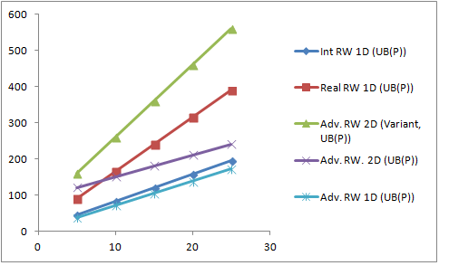
Figure 10: The plot of $\mathsf{UB}(P)$ vs the initial location.

Experimental results. Our experimental results are shown in Table 2 and Figure 10. Note that all examples considered, other than demonic RW in 2D, are in bounded LRApp (with no non-determinism or demonic non-determinism) for which all our results are polynomial time. For the demonic RW in 2D, which is not a bounded LRApp (for explanation why this is not a bounded LRApp see Section F of the appendix), concentration results cannot be obtained, however we obtain the upper bound $\mathsf{UB}(P)$ from our results as the example belongs to LRApp. Our experimental result show that the concentration bound and upper bound on expected termination time (recall $\mathsf{UB}(P)$ from Remark 6) we compute is a linear function in all cases (see Fig 10). This shows that our automated method can effectively compute, or some of the most classical random walks studied in probability theory, concentration bounds which are asymptotically tight (the expected number of steps to decrease the value of a standard asymmetric random walk by $n$ is equal to $n$ times the expected number of steps needed to decrease it by $1$, i.e. it is linear in $n$). For our experimental results, the linear constraints generated by LRSMSynth was solved by CPLEX cpl [2010]. The programs with the linear invariants are presented in Section F of the appendix.

Significance of our result. We now highlight the significance of our approach. The analysis of RW in 1D (even without adversary) is a classic problem in probability theory, and the expected termination time can be irrational and involve solving complicated equations. Instead our experimental results show that using our approach (which is polynomial time) we can compute upper bound on the expected time that is a linear function. This shows that we provide a practical and computational approach for quantitative reasoning of probabilistic processes. Moreover, our approach also extends to more complicated probabilistic processes (such as RW with adversary, as well as in 2D), and compute upper bounds which are linear, whereas precise mathematical analysis of such processes is extremely complicated.

7 Related Work

We have already discussed several related works, such as McIver and Morgan [2004, 2005]; Chakarov and Sankaranarayanan [2013]; Bournez and Garnier [2005]; Fioriti and Hermanns [2015] in Section 1 (Previous results). We discuss other relevant works here. The termination for concurrent probabilistic programs under fairness was considered in Sharir et al. [1984]. A sound and complete characterization of almost-sure termination for countable state space was given in Hart and Sharir [1985]. A sound and complete method for proving termination of finite state programs was given in Esparza et al. [2012]. Termination analysis of non-probabilistic programs has received a lot of attention over the last decade as well Bradley et al. [2005b]; Colón and Sipma [2001]; Podelski and Rybalchenko [2004]; Sohn and Gelder [1991]; Bradley et al. [2005a]; Cook et al. [2013]; Lee et al. [2001]. The most closely related works to our work are Chakarov and Sankaranarayanan [2013]; Bournez and Garnier [2005]; Fioriti and Hermanns [2015] that consider termination of probabilistic programs via ranking Lyapunov functions and supermartingales. However, most of the previous works focus on proving a.s. termination and finite termination, and discuss soundness and completeness. In contrast, in this work we consider simple (linear) ranking supermartingales, and study the related algorithmic and complexity issues. Moreover, we present answers to the quantitative termination questions, and also consider two types of non-determinism together that has not been considered before.

8 Conclusion and Future Work

In this work we considered the basic algorithmic problems related to qualitative and quantitative questions for termination of probabilistic programs. Since our focus was algorithmic we considered simple (linear) ranking supermartingales, and established several complexity results. The most prominent are that for programs with demonic non-determinism the qualitative problems can be solved in polynomial time, whereas for angelic non-determinism with no probability the qualitative problems are $\mathsf{NP}$-hard. We also present $\mathsf{PSPACE}$-hardness results for the quantitative problems, and present the first method through linear ranking supermartingales to obtain concentration results on termination time. There are several directions for future work. The first direction is to consider special cases of non-linear ranking supermartingales and study whether efficient algorithmic approaches can be developed for them. The second interesting direction would be to use the methods of martingale theory to infer deeper insights into the behaviour of probabilistic programs, e.g. via synthesizing assertions about the distribution of program variables (”stochastic invariants”).

Appendix A Proofs for Section 3

Proposition 1. Let $\{X_{n}\}_{n\in\mathbb{N}}$ be an RSM wrt filtration $\{\mathcal{F}_{n}\}_{n\in\mathbb{N}}$ and constants $K,\epsilon$ (cf. Definition 5). Let $Z$ be the random variable defined as $Z:=\min\{n\in\mathbb{N}\mid X_{n}<0\}$; which denotes the first time $n$ that the RSM $X_{n}$ drops below 0. Then $\mathbb{P}(Z<\infty)=1$ and $\mathbb{E}(Z)\leq\frac{\mathbb{E}(X_{1})-K}{\epsilon}$.

Proof.

The proof is similar to [Fioriti and Hermanns, 2015, Lemma 5.5]. We first prove by induction on $n\geq 1$ that

$$\mathbb{E}(X_{n})\leq\mathbb{E}(X_{1})-\epsilon\cdot\sum_{k=1}^{n-1}\mathbb{P}(X_{k}\geq 0)\enskip.$$

The base step $n=1$ is clear. The inductive step can be carried out as follows:

$$\begin{array}[]{rcl}\mathbb{E}(X_{n+1})&=&\mathbb{E}\left(\mathbb{E}(X_{n+1}\mid\mathcal{F}_{n})\right)\\[4.30554pt] &\leq&\mathbb{E}(X_{n})-\epsilon\cdot\mathbb{E}(\mathbf{1}_{X_{n}\geq 0})\\[4.30554pt] &\leq&\mathbb{E}(X_{1})-\epsilon\cdot\sum_{k=1}^{n-1}\mathbb{P}(X_{k}\geq 0)-\epsilon\cdot\mathbb{P}(X_{n}\geq 0)\\[4.30554pt] &=&\mathbb{E}(X_{1})-\epsilon\cdot\sum_{k=1}^{n}\mathbb{P}(X_{k}\geq 0)\enskip.\end{array}$$

The first equality is the total expectation law for conditional expectation; the first inequality is obtained from the fact that $X_{n}$ is a supermartingale; the second inequality is obtained from the inductive hypothesis; and the final equality is simply rearranging terms. Since $X_{n}\geq K$ almost surely for all $n\in\mathbb{N}$, we have that $\mathbb{E}(X_{n})\geq K$, for all $n$. Hence from above we have that

$$\sum_{k=1}^{n}\mathbb{P}(X_{k}\geq 0)\leq\frac{\mathbb{E}(X_{1})-\mathbb{E}(X_{n+1})}{\epsilon}\leq\frac{\mathbb{E}(X_{1})-K}{\epsilon}.$$

Hence the series $\sum_{k=1}^{\infty}\mathbb{P}(X_{k}\geq 0)$ converges and

$$\sum_{k=1}^{\infty}\mathbb{P}(X_{k}\geq 0)\leq\frac{\mathbb{E}(X_{1})-K}{\epsilon}\enskip.$$

It follows from $Z\geq k\Rightarrow X_{k}\geq 0$ that

• $\mathbb{P}(Z=\infty)=\lim_{k\rightarrow\infty}\mathbb{P}(Z\geq k)=0$ and

• $\mathbb{E}(Z)\leq\sum_{k=1}^{\infty}\mathbb{P}(X_{k}\geq 0)\leq\frac{\mathbb{E}(X_{1})-K}{\epsilon}$.

The desired result follows. ∎

To prove Theorem 1, we need the following lemma which specifies the relationship between pre-expectation and conditional expectation.

Lemma 6.

Let $\eta$ be an LRSM and $\sigma$ be the angelic scheduler whose decisions optimize the value of $\eta$ at the last configuration of any finite path, represented by

$$\sigma(\ell,\mathbf{x})=\mathrm{argmin}_{(\ell,f,\ell^{\prime})\in\mapsto}\eta(\ell^{\prime},\mathbf{x})$$

for all end configuration $(\ell,\mathbf{x})$ such that $\ell\in L_{A}$ and $\mathbf{x}\in\mathbb{R}^{|X|}$. Let $\pi$ be any demonic scheduler. Let the stochastic process $\{X_{n}\}_{n\in\mathbb{N}}$ be defined such that

$$X_{n}:=\eta(\theta_{n},\{\overline{x}_{k,n}\}_{1\leq k\leq|X|})\enskip.$$

Then for all $n\in\mathbb{N}$,

$$\mathbb{E}^{\sigma,\pi}(X_{n+1}\mid\mathcal{F}_{n})\leq\mathrm{pre}_{\eta}(\theta_{n},\{\overline{x}_{k,n}\}_{1\leq k\leq|X|})\enskip.$$

Proof.

For all $n\in\mathbb{N}$, from the program syntax we have

$$X_{n+1}=\mathbf{1}_{\theta_{n}=\ell_{p}^{\mathit{out}}}\cdot X_{n}+Y_{P}+Y_{S}+Y_{A}+Y_{D}$$

where the terms are described below:

$$Y_{P}:=\sum_{\ell\in L_{P}}\Big{[}\mathbf{1}_{\theta_{n}=\ell}\cdot\sum_{i\in\{0,1\}}\big{(}\mathbf{1}_{B_{\ell}=i}\cdot\eta(\ell_{B_{\ell}=i},\{\overline{x}_{k,n}\}_{k})\Big{]}$$

where each random variable $B_{\ell}$ is the Bernoulli random variable for the decision of the probabilistic branch and $\ell_{B_{\ell}=0},\ell_{B_{\ell}=1}$ are the corresponding successor locations of $\ell$. Note that all $B_{\ell}$’s and $\mathbf{r}$’s are independent of $\mathcal{F}_{n}$. In other words, $Y_{P}$ describes the semantics of probabilistic locations.

$$Y_{S}:=\sum_{\ell\in L_{S}}\sum_{(\ell,f,\ell^{\prime})\in\mapsto_{\ell}}\Big{[}\mathbf{1}_{\theta_{n}=\ell\wedge\{\overline{x}_{k,n}\}_{k}\in G(\tau)}\cdot\eta(\ell^{\prime},f(\{\overline{x}_{k,n}\}_{k},\mathbf{r})\Big{]};$$

describes the semantics of deterministic locations.

$$Y_{A}:=\sum_{\ell\in L_{A}}\mathbf{1}_{\theta_{n}=\ell}\cdot\eta(\sigma(\ell,\{\overline{x}_{k,n}\}_{k}),\{\overline{x}_{k,n}\}_{k});$$

describes the semantics of angelic locations, where $\sigma(\ell,\{\overline{x}_{k,n}\}_{k})$ here denotes the target location of the transition chosen by the scheduler; and similarly, for demonic locations by replacing $\sigma$ by $\pi$ we have

$$Y_{D}:=\sum_{\ell\in L_{D}}\mathbf{1}_{\theta_{n}=\ell}\cdot\eta(\pi(\rho),\{\overline{x}_{k,n}\}_{k}),$$

where $\rho$ is the finite path up to $n$ steps. Then from properties of conditional expectation [Williams, 1991, Page 88], one obtains:

$$\mathbb{E}^{\sigma,\pi}(X_{n+1}\mid\mathcal{F}_{n})=\mathbf{1}_{\theta_{n}=\ell_{p}^{\mathit{out}}}\cdot X_{n}+Y^{\prime}_{P}+Y^{\prime}_{S}+Y_{A}+Y_{D},$$

because $\mathbf{1}_{\theta_{n}=\ell_{p}^{\mathit{out}}}\cdot X_{n}$, $Y_{A}$, $Y_{D}$ are measurable in $\mathcal{F}_{n}$, we have $\mathbb{E}^{\sigma,\pi}(\mathbf{1}_{\theta_{n}=\ell_{p}^{\mathit{out}}}\cdot X_{n}\mid\mathcal{F}_{n})=\mathbf{1}_{\theta_{n}=\ell_{p}^{\mathit{out}}}\cdot X_{n}$ (and similarly for $Y_{A}$ and $Y_{D}$); and for $Y_{P}$ and $Y_{S}$ we need their expectation as $Y_{P}^{\prime}$ and $Y_{S}^{\prime}$ defined below. We have

$$Y^{\prime}_{P}:=\sum_{\ell\in L_{P}}\Big{[}\mathbf{1}_{\theta_{n}=\ell}\cdot\sum_{i\in\{0,1\}}\big{(}\mathbb{P}(B_{\ell}=i)\cdot\eta(\ell_{B_{\ell}=i},\{\overline{x}_{k,n}\}_{k})\big{)}\Big{]}$$

$$Y^{\prime}_{S}:=\sum_{\ell\in L_{S}}\sum_{(\ell,f,\ell^{\prime})\in\mapsto_{\ell}}\Big{[}\mathbf{1}_{\theta_{n}=\ell\wedge\{\overline{x}_{k,n}\}_{k}\models G(\tau)}\cdot\eta(\ell^{\prime},\mathbb{E}^{\sigma,\tau}_{R}\left(f(\{\overline{x}_{k,n}\}_{k},\mathbf{r})\right)\Big{]}\enskip.$$

Note that when $\theta_{n}\in L_{S}\cup L_{P}\cup L_{A}$, by definition we have $\mathrm{pre}_{\eta}(\theta_{n},\{\overline{x}_{k,n}\}_{k})=\mathbf{1}_{\theta_{n}=\ell_{p}^{\mathit{out}}}\cdot X_{n}+Y^{\prime}_{P}+Y^{\prime}_{S}+Y_{A}$; and when $\theta_{n}\in L_{D}$ by definition we have $Y_{D}\leq\mathrm{pre}_{\eta}(\theta_{n},\{\overline{x}_{k,n}\}_{k})$. Hence the result follows. ∎

Theorem 1. If there exists an LRSM $\eta$ wrt $I$ for $\mathcal{G}_{P}$, then

1. $P$ is a.s. terminating; and

2. the expected termination time of $P$ is at most $\frac{\eta(\ell_{0},\mathbf{x}_{0})-K^{\prime}}{\epsilon}$ and hence finite, i.e., $\mathsf{ET}(P)<\infty$.

Proof.

We establish both the points. Let $\eta$ be an LRSM wrt $I$ for $\mathcal{G}_{P}$. Define the angelic strategy $\sigma$ which solely depends on the end configuration of a finite path as follows:

$$\sigma(\ell,\mathbf{x})=\mathrm{argmin}_{(\ell,f,\ell^{\prime})\in\mapsto}\eta(\ell^{\prime},\mathbf{x})$$

for all $\ell\in L_{A}$ and $\mathbf{x}\in\mathbb{R}^{|X|}$. Fix any demonic strategy $\pi$. Let the stochastic process $\{X_{n}\}_{n\in\mathbb{N}}$ be defined by:

$$X_{n}:=\eta(\theta_{n},\{\overline{x}_{k,n}\}_{k}).$$

For all $n\in\mathbb{N}$, from Lemma 6, we have

$$\mathbb{E}^{\sigma,\pi}(X_{n+1}\mid\mathcal{F}_{n})\leq\mathrm{pre}_{\eta}(\theta_{n},\{\overline{x}_{k,n}\}_{k})\enskip.$$

By condition C4,

$$\mathrm{pre}_{\eta}(\theta_{n},\{\overline{x}_{k,n}\}_{k})\leq\eta(\theta_{n},\{\overline{x}_{k,n}\}_{k})-\epsilon\cdot\mathbf{1}_{\theta_{n}\neq\ell_{P}^{\mathit{out}}}$$

for some $\epsilon\geq 1$. Moreover, from C2, C3 and the fact that $I$ is a linear invariant, it holds almost-surely that $\theta_{n}\neq\ell_{P}^{\mathit{out}}$ iff $X_{n}\geq 0$. Thus, we have

$$\mathbb{E}^{\sigma,\pi}(X_{n+1}\mid\mathcal{F}_{n})\leq X_{n}-\epsilon\cdot\mathbf{1}_{X_{n}\geq 0}\enskip.$$

It follows that $\{X_{n}\}_{n\in\mathbb{N}}$ is an RSM. Hence by Proposition 1, it follows that $\mathcal{G}_{P}$ terminates almost surely and

$$\mathbb{E}^{\sigma,\pi}(T)\leq\frac{\eta(\ell_{0},\mathbf{x}_{0})-K^{\prime}}{\epsilon}\enskip.$$

The desired result follows. ∎

Appendix B Proofs for Section 4.1

Lemma 1. Let $\mathbf{A}\in\mathbb{R}^{m\times n}$, $\mathbf{B}\in\mathbb{R}^{k\times n}$, $\mathbf{b}\in\mathbb{R}^{m}$, $\mathbf{d}\in\mathbb{R}^{k}$, $\mathbf{c}\in\mathbb{R}^{n}$ and $d\in\mathbb{R}$. Let $\mathbf{Z}_{<}=\{\mathbf{x}\mid\mathbf{A}\mathbf{x}\leq\mathbf{b}\wedge\mathbf{B}\mathbf{x}<\mathbf{d}\}$ and $\mathbf{Z}_{\leq}=\{\mathbf{x}\mid\mathbf{A}\mathbf{x}\leq\mathbf{b}\wedge\mathbf{B}\mathbf{x}\leq\mathbf{d}\}$. Assume that $\mathbf{Z}_{<}\neq\emptyset$. Then for all closed subsets $H\subseteq\mathbb{R}^{|X|}$ we have that $\mathbf{Z}_{<}\subseteq H$ implies $\mathbf{Z}_{\leq}\subseteq H$.

Proof.

Let $\mathbf{z}$ be any point such that $\mathbf{A}\mathbf{z}\leq\mathbf{b}$, $\mathbf{B}\mathbf{z}\leq\mathbf{d}$ and $\mathbf{B}\mathbf{z}\not<\mathbf{d}$. Let $\mathbf{y}$ be a point such that $\mathbf{A}\mathbf{y}\leq\mathbf{b}$ and $\mathbf{B}\mathbf{y}<\mathbf{d}$. Then for all $\lambda\in(0,1)$,

$$\lambda\cdot\mathbf{y}+(1-\lambda)\cdot\mathbf{z}\in\{\mathbf{x}\mid\mathbf{A}\mathbf{x}\leq\mathbf{b}\wedge\mathbf{B}\mathbf{x}<\mathbf{d}\}\enskip.$$

By letting $\lambda\rightarrow 1$, we obtain that $\mathbf{z}\in H$ because $H$ is closed. ∎

Lemma 2. Let $\mathbf{A}\in\mathbb{R}^{m\times n}$, $\mathbf{B}\in\mathbb{R}^{k\times n}$, $\mathbf{b}\in\mathbb{R}^{m}$ and $\mathbf{d}\in\mathbb{R}^{k}$. Then all of the following three problems can be decided in polynomial time in the binary encoding of $\mathbf{A},\mathbf{B},\mathbf{b},\mathbf{d}$:

1. $\{\mathbf{x}\mid\mathbf{A}\mathbf{x}\leq\mathbf{b}\}\stackrel{{\scriptstyle?}}{{=}}\emptyset$;

2. $\{\mathbf{x}\mid\mathbf{A}\mathbf{x}\leq\mathbf{b}\wedge\mathbf{B}\mathbf{x}<\mathbf{d}\}\stackrel{{\scriptstyle?}}{{=}}\emptyset$;

3. $\{\mathbf{x}\mid\mathbf{B}\mathbf{x}<\mathbf{d}\}\stackrel{{\scriptstyle?}}{{=}}\emptyset$.

Proof.

The polynomial-time decidability of the first problem is well-known (cf.  Schrijver [1999]). The second problem can be solved by checking whether the optimal value of the following linear program is greater than zero:

$$\max z\text{ subject to }\mathbf{A}\mathbf{x}\leq\mathbf{b};\quad\mathbf{B}\mathbf{x}+z\cdot\mathbf{1}\leq\mathbf{d};\quad z\geq 0.$$

The proof for the third problem is similar to the second one. ∎

Appendix C Proofs for Section 4.2

Lemma 3. The LRApp realizability problem for Apps with angelic non-determinism is $\mathsf{NP}$-hard, even for non-probabilistic non-demonic programs with simple guards.

Proof.

We show a polynomial reduction from $3$-SAT to the LRApp realizability problem.

Let $\psi$ be any propositional formula in a conjunctive normal form with three literals per clause. Let $C_{1},\dots,C_{m}$ be all the clauses and $x_{1},\dots,x_{n}$ all the variables of $\psi$. For every $1\leq j\leq m$ we write $C_{j}\equiv\xi_{j,1}\vee\xi_{j,2}\vee\xi_{j,3}$, where each $\xi_{j,k}$ is either a positive or a negative literal, i.e. a variable or its negation.

We construct a program $P_{\psi}$ as follows: the program variables of $P_{\psi}$ correspond to the variables in $\psi$, the program has no random variables. All the program variables are initially set to 1. To construct the body of the program, we define, for each literal $\xi$ of $\psi$ involving a variable $x_{i}$, a linear expression $g_{\xi}$ which is equal either to $x_{i}$ or $1-x_{i}$ depending on whether $\xi$ is a positive literal or not, respectively. The body of the program then has the form

$$\mathbf{while}~{}\varphi~{}\mathbf{do}~{}Q_{1};\cdots;Q_{n}~{}\mathbf{od}$$

where

• $\varphi$ is a finite disjunction of linear constraints of the form

  $$\bigvee_{j=1}^{m}\left[g_{\xi_{j,1}}+g_{\xi_{j,2}}+g_{\xi_{j,3}}\leq\frac{1}{2}\right]\enskip;$$

• $Q_{i}$ has the form if angel then $x_{i}:=1$ else $x_{i}:=0$ fi, for all $1\leq i\leq n$.

Clearly, given a formula $\psi$ the program $P_{\psi}$ can be constructed in time polynomial in the size of $\psi$, and moreover, $P_{\psi}$ is non-probabilistic and non-demonic.

Note that each valuation $\mathbf{x}$, reachable from the initial configuration of $\mathcal{G}_{P_{\psi}}$, can be viewed as a bit vector, and hence we can identify these reachable valuations with truth assignments to $\psi$. Also note that for such a reachable valuation $\mathbf{x}$ it holds $g_{\xi_{j,k}}(\mathbf{x})=1$ if and only if $\mathbf{x}$, viewed as an assignment, satisfies the formula $\xi_{j,k}$, and $g_{\xi_{j,k}}(\mathbf{x})=0$ otherwise.

Finally, let $I$ be an invariant assigning to every location a linear assertion $\bigwedge_{i=1}^{n}[0\leq x_{i}\wedge x_{i}\leq 1]$. Note that the invariant $I$ is very simple and it is plausible that it can be easily discovered without employing any significant insights into the structure of $P_{\psi}$.

We claim that $P_{\psi}$ admits a linear ranking supermartingale with respect to $I$ if and only if there exists a satisfying assignment for $\psi$. First let us assume that $\psi$ is not satisfiable. Then, as noted above, for all reachable valuations $\mathbf{x}$ there is $1\leq j\leq m$ such that for all $\xi_{j,k}$, $1\leq k\leq 3$, it holds $g_{\xi_{j,k}}(\mathbf{x})=0$. It follows that $\varphi$ holds in every reachable valuation and hence the program never terminates. From Theorem 1 it follows that $P_{\psi}$ does not admit an LRSM for any invariant $I$.

Let us now assume that there exists an assignment $\nu\colon\{x_{1},\dots,x_{n}\}\rightarrow\{0,1\}$ satisfying $\psi$. We use $\nu$ to construct an LRSM for $P_{\psi}$ with respect to $I$. First, let us fix the following notation of locations of $\mathcal{G}_{P_{\psi}}$: by $\ell_{i}$ we denote the initial location of the sub-program $Q_{i}$, by $\ell_{i}^{1}$ and $\ell_{i}^{0}$ the locations corresponding to ”then” and ”else” branches of $Q_{i}$, respectively, and by $\ell_{n+1}$ and $\ell^{\mathit{out}}$ the initial and terminal locations of $\mathcal{G}_{P_{\psi}}$, respectively. Next, we fix a penalty constant $\mathit{Pen}=4n+3$ and for every pair of indexes $1\leq i\leq n+1$, $1\leq j\leq n$ we define a linear expression

$$h_{i,j}=\begin{dcases}1-x_{j}&\text{if }\nu(x_{j})=1\text{ and }i\leq j,\\ (1-x_{j})\cdot\mathit{Pen}&\text{if }\nu(x_{j})=1\text{ and }i>j,\\ x_{j}&\text{if }\nu(x_{j})=0\text{ and }i\leq j,\\ x_{j}\cdot\mathit{Pen}&\text{if }\nu(x_{j})=0\text{ and }i>j.\end{dcases}$$

Note that for $\mathbf{x}\in[0,1]^{n}$ the value $h_{i,j}(\mathbf{x})$ equals either $|\nu(x_{j})-\mathbf{x}[j]|$ or $|\nu(x_{j})-\mathbf{x}[j]|\cdot\mathit{Pen}$ depending on whether $i\leq j$ or not.

Finally, we define an LRSM $\eta$ as follows: for every $1\leq i\leq n+1$ we put

$$\eta(\ell_{i},\mathbf{x}) =\sum_{j=1}^{n}h_{i,j}(\mathbf{x})+(n-i+1)\cdot 2.$$

Next, for every $1\leq i\leq n$ we put

$$\eta(\ell_{i}^{\nu(x_{i})},\mathbf{x}) =\sum_{j=1}^{n}h_{i,j}(\mathbf{x})+(2(n-i)+1)$$

$$\eta(\ell_{i}^{1-\nu(x_{i})},\mathbf{x}) =n\cdot\mathit{Pen}+2n+1.$$

Finally, we put $\eta(\ell^{\mathit{out}},\mathbf{x})=-1/2$.

We show that $\eta$ is an LRSM wrt $I$.

As $h_{i,j}(\mathbf{x})\geq 0$ whenever $\mathbf{x}\in[0,1]^{n}$, it is easy to check that $\mathbf{x}\in\bigcup I(\ell)\Rightarrow\eta(\ell,\mathbf{x})\geq 0$ for every non-terminal location $\ell$. Next, for each $\mathbf{x}\in\mathbb{R}^{n}$ and each angelic state $\ell_{i}$ it holds that $\eta(\ell_{i},\mathbf{x})=\eta(\ell_{i}^{\nu(x_{i})},\mathbf{x})+1$; hence $\mathrm{pre}_{\eta}(\ell_{i},\mathbf{x})\leq\eta(\ell_{i},\mathbf{x})-1$. Further, let us observe that for all $\mathbf{x}\in[0,1]^{n}$ and all $1\leq i\leq n+1$ we have $\eta(\ell_{i},\mathbf{x})\leq n\cdot\mathit{Pen}+2n$; thus for all $1\leq i\leq n$ it holds that $\mathrm{pre}_{\eta}(\ell_{i}^{1-\nu(x_{i})},\mathbf{x})\leq\eta(\ell_{i}^{1-\nu(x_{i})},\mathbf{x})-1$. Also, for all such $\mathbf{x}$ and $i$ it holds that

$$\eta(\ell_{i}^{\nu(x_{i})},\mathbf{x})$$

$$= \eta(\ell_{i+1},[x_{i}/\nu(x_{i})](\mathbf{x}))+h_{i,i}(\mathbf{x})$$

$$\quad{}-h_{i,i+1}([x_{i}/\nu(x_{i})](\mathbf{x}))+1$$

$$\geq \eta(\ell_{i+1},[x_{i}/\nu(x_{i})](\mathbf{x}))+1\enskip,$$

where the latter inequality follows from $h_{i,i+1}([x_{i}/\nu(x_{i})](\mathbf{x}))=0$ and non-negativity of $h_{i,i}(\mathbf{x})$ for $\mathbf{x}\in[0,1]^{n}$. Hence, $\mathrm{pre}_{\eta}(\ell_{i}^{\nu(x_{i})},\mathbf{x})\leq\eta(\ell_{i}^{\nu(x_{i})},\mathbf{x})-1$. Finally, let us focus on $\ell_{n+1}$. Let $\mathbf{x}$ be such that $\mathbf{x}\models\varphi\wedge I(\ell_{n+1})$. It is easy to check that

$$\mathrm{pre}_{\eta}(\ell_{n+1},\mathbf{x})=\eta(\ell_{n+1},\mathbf{x})+2n-(\mathit{Pen}-1)\cdot\sum_{i=1}^{n}|\nu(x_{i})-\mathbf{x}[i]|.$$ (1)

Now since $\mathbf{x}\models\varphi$, there is $1\leq j\leq m$ such that $(g_{\xi_{j,1}}+g_{\xi_{j,2}}+g_{\xi_{j,3}})(\mathbf{x})\leq\frac{1}{2}$, which implies $g_{\xi_{j,k}}(\mathbf{x})\leq\frac{1}{2}$ for all $1\leq k\leq 3$, as all these numbers are non-negative. On the other hand, there is $1\leq k^{\prime}\leq 3$ such that $\nu(\xi_{j,k^{\prime}})=1$, as $\nu$ is a satisfying assignment. Let $x_{i}$ be the variable in $\xi_{j,k^{\prime}}$. If $\xi_{j,k^{\prime}}$ is a positive literal, then $\nu(x_{i})=1$ and $\mathbf{x}[i]=g_{\xi_{j,k^{\prime}}}(\mathbf{x})\leq\frac{1}{2}$, and if $\xi_{j,k^{\prime}}$ is negative, then $\nu_{x_{i}}=0$ and $\mathbf{x}[i]=1-g_{\xi_{j,k^{\prime}}}(\mathbf{x})\geq\frac{1}{2}$. In both cases we get $|\nu(x_{i})-\mathbf{x}[i]|\geq\frac{1}{2}$. Plugging this into (1) and combining with the fact that $(\mathit{Pen}-1)/2\geq 2n+1$ we get that $\mathrm{pre}_{\eta}(\ell_{n+1},\mathbf{x})\leq\eta(\ell_{n+1},\mathbf{x})-1$. Hence, $\eta$ is indeed an LRSM. ∎

Appendix D Details of Section 5

D.1 Irrationality of expected termination time

Let us again consider the program $P$ in Figure 9. We claim that $\mathsf{ET}(P)$ is irrational. Note that the stochastic game structure $\mathcal{G}_{P}$ has six locations, where the following two are of interest for us: the location corresponding to the beginning of the while loop, which we denote by while, and the location entered after executing the first assignment in the else branch, which we denote by else. Consider the following systems of polynomial equations:

$$x_{\textit{while},\textit{while}} =\frac{1}{2}(x_{\textit{while},\textit{while}}^{2}+x_{\textit{while},\textit{else}})$$

$$x_{\textit{while},\textit{else}} =\frac{1}{2}+\frac{1}{2}(x_{\textit{while},\textit{while}}\cdot x_{\textit{while},\textit{else}})$$

$$y_{\textit{while},\textit{while}} =\frac{\frac{1}{2}(3+2y_{\textit{while},\textit{while}}\cdot x^{2}_{\textit{while},\textit{while}}+(y_{\textit{while},\textit{else}}+1)\cdot x_{\textit{while},\textit{else}})}{x_{\textit{while},\textit{while}}}$$

$$y_{\textit{while},\textit{else}} =\frac{\frac{3}{2}+\frac{1}{2}(3+y_{\textit{while},\textit{while}}+y_{\textit{while},\textit{else}})\cdot x_{\textit{while},\textit{while}}\cdot x_{\textit{while},\textit{else}}}{x_{\textit{while},\textit{else}}}$$

Intuitively, the variable $x_{\ell,\ell^{\prime}}$ represents the probability that when starting in location $\ell$ with variable $n$ having some value $k$, the first location in which the value of $n$ decreases to $k-1$ is $\ell^{\prime}$ (note that this probability is independent of $k$). Next, $y_{\ell,\ell^{\prime}}$ is the conditional expected number of steps needed to decrease $n$ by 1, conditioned by the event that we start in $\ell$ and the first state in which $n$ drops below the initial value is $\ell^{\prime}$. Formally, it is shown in Brázdil et al. [2012] and Esparza et al. [2005] that these probabilities and expectations are the minimal non-negative solutions of the system.

It is then easy to check that the expected termination time of $P$ is given by the formula

$$1+x_{\textit{while},\textit{while}}(y_{\textit{while},\textit{while}}+1)+x_{\textit{while},\textit{else}}(y_{\textit{while},\textit{else}}+2).$$ (3)

Examining the solutions of (LABEL:eq:system) (we used Wolfram Alpha to identify them) we get that $x_{\textit{while},\textit{while}}=\frac{3-\sqrt{5}}{2}$, $x_{\textit{while},\textit{else}}=\frac{\sqrt{5}-1}{2}$, $y_{\textit{while},\textit{while}}=(85+43\sqrt{5})/10$, $y_{\textit{while},\textit{else}}=(15+29\sqrt{5})/10$. Plugging this into (3) we get that $\mathsf{ET}(P)=2(5+\sqrt{5})$.

D.2 Proof of Lemma 4

Lemma 4. The quantitative approximation problem can be solved in a doubly exponential time for programs with only discrete probability choices.

Proof.

The algorithm proceeds via analysing a suitable finite unfolding of the input program $P$. Formally, an $n$-step unfolding of $P$, where $n\in\mathbb{N}$, is an SGS $\mathit{Unf}(P,n)$ such that

• the set locations of $\mathit{Unf}(P,n)$ consists of certain finite paths in $\mathcal{G}_{P}$ (i.e. in the SGS associated to $P$). Namely, we take those finite paths whose starting configuration is the initial configuration of $\mathcal{G}_{P}$ and whose length is at most $n$. The type of such a location $w$ is determined by the type of a location in the last configuration of $\mathcal{G}_{P}$ appearing on $w$.

• $\mathit{Unf}(P,n)$ has the same program and random variables as $\mathcal{G}_{P}$ (i.e. the same ones as $P$) and the initial configuration of $\mathit{Unf}(P,n)$ is the tuple $((\ell_{0},\mathbf{x}_{0}),\mathbf{x}_{0})$, where $(\ell_{0},\mathbf{x}_{0})$ is the initial configuration of $\mathcal{G}_{P}$ (it can be identified with a finite path of length 0).

• For every pair $w$, $w^{\prime}$ of locations of $\mathit{Unf}(P,n)$ (i.e., $w$, $w^{\prime}$ are finite paths in $\mathcal{G}_{P}$) such that $w^{\prime}$ can be formed by performing a single transition $\tau$ out of the last configuration of $w$, there is a transition $(w,f,w^{\prime})$ in $\mathit{Unf}(P,n)$, where $f$ is an update function of $\tau$. Moreover, for every history $w$ of length $n$ that is also a location of $\mathit{Unf}(P,n)$ there is a transition $(w,\mathit{id},w)$ in $\mathit{Unf}(P,n)$.

• The probability distributions and guard functions for probabilistic/deterministic locations $w$ of $\mathit{Unf}(P,n)$ are determined, in a natural way, by the probability distribution/guard functions of the location in the last configuration of $w$.

Note that that each configuration of $\mathit{Unf}(P,n)$ reachable from the initial configuration is of the form $((\ell_{0},\mathbf{x}_{0}),\dots,(\ell_{i},\mathbf{x}_{i}),\mathbf{x}_{i})$, where $(\ell_{j},\mathbf{x}_{j}),0\leq j\leq i$ are configurations of $\mathit{Unf}(P,n)$. In particular, the values of program variables in every reachable configuration $(w,\mathbf{x})$ of $\mathit{Unf}(P,n)$ are uniquely determined by $w$. To avoid confusion, in the following we will denote the locations in $\mathcal{G}_{P}$ by $\ell,\ell_{0},\ell_{1},\dots$ and locations in $\mathit{Unf}(P,n)$ by $w,w_{0},w_{1},\dots$.

Given $P$ and $n$ it is possible to construct $\mathit{Unf}(P,n)$ in time exponential in $n$ and in the encoding size of $P$. To see this, observe that the graph of $\mathit{Unf}(P,n)$ is a tree of depth $n$ and so $\mathit{Unf}(P,n)$ has at most $2^{n}$ locations. We can construct $\mathit{Unf}(P,n)$ by, e.g. depth-first enumeration of all finite paths in $\mathcal{G}_{P}$ of length $\leq n$. To bound the complexity of the construction we need to bound the magnitude of numbers (i.e. variable values) appearing on these finite paths – these are needed to determine which transition to take in deterministic locations. Note that for every App $P$ there is a positive number $K$ at most exponential in the encoding size of $P$ such that in every step the absolute value of any variable of $P$ can increase by the factor of at most $K$ in every step. Hence, after $n$ steps the absolute value of every variable is bounded by $K^{n}\cdot L$, where $L$ is a maximal absolute value of any variable of $P$ upon initialization ($L$ is again at most exponential in the size of $P$). The exponential (in $n$ and size of $P$) bound on the time needed to construct $\mathit{Unf}(P,n)$ follows.

After constructing $\mathit{Unf}(P,n)$, we post-process the SGS by removing all transitions outgoing from angelic locations that violate the supermartingale property of $\eta$. Formally, for every angelic location $w$ of $\mathit{Unf}(P,n)$ and each its successor $w^{\prime}$ we denote by $c$ and $c^{\prime}$ the last configurations on $w$ and $w^{\prime}$, respectively. We then check whether $\mathrm{pre}_{\eta}(c)=\eta(c^{\prime})$, and if not, we remove the transition from $w$ to $w^{\prime}$.

There is a natural many-to-one surjective correspondence $\Gamma$ between demonic schedulers in $\mathcal{G}_{P}$ and demonic schedulers in $\mathit{Unf}(P,n)$ (the schedulers in $\mathcal{G}_{P}$ that have the same behaviour up to step $n$ are mapped to a unique scheduler in $\mathit{Unf}(P,n)$ which induces this behaviour). Similarly, there is a many-to-one correspondence $\Delta$ between angelic schedulers that belong to $\mathit{cmp(\eta)}$ in $\mathcal{G}_{P}$ and angelic schedulers in $\mathit{Unf}(P,n)$.

Let $Term_{n}$ be the set of all locations $w$ in $\mathit{Unf}({P},n)$ that, when interpreted as paths in $\mathcal{G}_{P}$, end with a configuration of the form $(\ell_{P}^{\mathit{out}},\mathbf{x})$ for some $\mathbf{x}$. It is easy to verify that for any adversarial scheduler $\pi$ in $\mathcal{G}_{P}$ the probability $\mathbb{P}^{\pi}(T\leq x))$ is equal to the probability of reaching $Term_{n}$ under $\Phi(\pi)$ in $\mathit{Unf}(P,n)$.

To solve the quantitative approximation problem we proceed as follows: First we compute number $n$, at most exponential in the size of $P$, such that the infimum (among all angelic schedulers in $\mathit{cmp(\eta)}$) probability of not terminating in the first $n$ steps is ”sufficiently small” in $\mathcal{G}_{P}$. Then we construct, in time exponential in $n$ and size of $P$ the unfolding $\mathit{Unf}(P,n)$ and assign a non-negative cost $cost(w)$ to each location $w$ of $\mathit{Unf}(P,n)$. We then define a random variable $W$ which to each run $(w_{0},\mathbf{x}_{0}),(w_{1},\mathbf{x}_{1}),\dots$ in $\mathit{Unf}(P,n)$ assigns the number $\sum_{i=0}^{j}cost(w_{i})$, where $j=\min\{n,\min\{k\mid w_{k}\in Term_{n}\}\}$. Using the fact that in $\mathcal{G}_{P}$ we terminate with very high probability in the first $n$ steps, we will show how to construct the cost function $cost$ in such a way that for every pair of schedulers $\sigma,\pi$, where $\sigma\in\mathit{cmp(\eta)}$, it holds $|\mathbb{E}^{\sigma,\pi}T-\mathbb{E}^{\Delta(\sigma),\Gamma(\pi)}W|\leq\delta$ (the construction of $cost$ can be done in time polynomial in the size of $\mathit{Unf}(P,n)$). Hence, to solve the quantitative approximation problem it will suffice to compute $\inf_{\sigma^{\prime}}\sup_{\pi^{\prime}}\mathbb{E}^{\sigma^{\prime},\pi^{\prime}}W$, where the infimum and supremum are taken over schedulers in $\mathit{Unf}(P,n)$. This computation can be done in polynomial time via standard backward iteration Osborne and Rubinstein [1994]. The doubly-exponential bound then follows from the aforementioned bound on the size of $\mathit{Unf}(P,n)$.

First let us show how to compute $n$. Since $P$ is a bounded LRAppand we are given the corresponding ranking supermartingale $\eta$ with one-step change bounds $a,b$, by Theorem 5 we can compute, in polynomial time, a concentration bound $B$ which is at most exponential in the size of $P$. That is, there are positive numbers $c_{1}$, $c_{2}$, which depend just on $P$, such that for each $x\geq B$ it holds $\mathsf{Thr}(P,x)\leq c_{1}\cdot\exp(-c_{2}\cdot x)$. Moreover, numbers $c_{1}$ and $c_{2}$ are also computable in polynomial time and at most exponential in the size of $P$, as witnessed in the proof of Theorem 5. Now denote by $M_{0}$ the value of the LRSM $\eta$ in the initial configuration of $P$. Note that $M_{0}$, as well as the bounds $a$, $b$, are at most exponential in the size of $P$ as $\eta$, $a$ and $b$ can be obtained by solving a system of linear inequalities with coefficients determined by $P$. We compute (in polynomial time) the smallest integer $n\geq B$ such that $c_{1}\cdot e^{-c_{2}\cdot n}\cdot(n+(M_{0}+n\cdot(b-a))/\epsilon)\leq\delta$, where $\epsilon$ is as in Definition 8 (the minimal expected decrease of the value of $\eta$ in a single step). It is straightforward to verify that such an $n$ exists and that it is polynomial in $M_{0}$, $\epsilon$, and $a,b$, and hence exponential in the size of $P$.

Now let us construct the cost function $cost$. The initial location gets cost 0 and all other locations get cost 1 except for locations $w$ that represents the paths in $\mathcal{G}_{P}$ of lenth $n$. The latter locations get a special cost $C=(M_{0}+n\cdot(b-a))/\epsilon$.

We prove that for any pair of schedulers $\sigma,\pi$, $\sigma\in\mathit{cmp(\eta)}$, it holds $|\mathbb{E}^{\sigma,\pi}T-\mathbb{E}^{\Delta(\sigma),\Gamma(\pi)}W|\leq\delta$. So fix an arbitrary such pair. We start by proving that $\mathbb{E}^{\sigma,\pi}T\leq\mathbb{E}^{\Delta(\sigma),\Gamma(\pi)}W$. Since the behaviour of the schedulers in the first $n$ steps is mimicked by $\Delta(\sigma)$ and $\Gamma(\pi)$ in $\mathit{Unf}(P,n)$, and in the latter SGS we accumulate one unit of cost per each of the first $n-1$ steps, it suffices to show that the expected number of steps needed to terminate with these schedulers from any configuration of $\mathcal{G}_{P}$ that is reachable in exactly $n$ steps is bounded by $C$. Since the value of $\eta$ can change by at most $(b-a)$ in every step, and $\sigma\in\mathit{cmp(\eta)}$, the value of $\eta$ after $n$ steps in $\mathcal{G}_{P}$ is at most $M_{0}+n\cdot(b-a)$. By Theorem 1 the expected number of step to terminate from a configuration with such an $\eta$-value is at most $(M_{0}+n\cdot(b-a))/\epsilon$ as required.

To finish the proof we show that $\mathbb{E}^{\Delta(\sigma),\Gamma(\pi)}W\leq\mathbb{E}^{\sigma,\pi}T+\delta$. First note that $\mathbb{E}^{\Delta(\sigma),\Gamma(\pi)}W-\mathbb{E}^{\sigma,\pi}T$ can be bounded by $p\cdot C$, where $p$ is the probability that a run in $\mathcal{G}_{P}$ does not terminate in first $n$ steps under these schedulers. Since $n\geq B$ it holds $p\leq c_{1}\cdot e^{-c_{2}\cdot n}$. Thus $p\cdot C\leq c_{1}\cdot e^{-c_{2}\cdot n}\cdot(n+(M_{0}+n\cdot(b-a))/\epsilon)\leq\delta$, the last inequality following from the choice of $n$.

∎

D.3 Proofs for Section 5.2

Lemma 5. For every $C\in\mathbb{N}$ the following problem is $\mathsf{PSPACE}$-hard: Given a program $P$ without probability or non-determinism, with simple guards, and belonging to bounded LRApp; and a number $N\in\mathbb{N}$ such that either $\mathsf{ET}(P)\leq N$ or $\mathsf{ET}(P)\geq N\cdot C$, decide, which of these two alternatives hold.

Proof.

Let us fix a constant $C$.

We start by noting that there exists a constant $K$ such that the following $K$-linearly bounded membership problem is $\mathsf{PSPACE}$-hard: Given a deterministic Turing machine (DTM) $\mathcal{T}$ such that on every input of length $n$ the machine $\mathcal{T}$ uses at most $K\cdot n$ tape cells, and given a word $w$ over the input alphabet of $\mathcal{T}$, decide, whether $\mathcal{T}$ accepts $w$. This is because there exists $K$ for which there is a DTM $\mathcal{T}_{\textsc{QBF}}$ satisfying the above condition which decides the QBF problem ($\mathcal{T}_{\textsc{QBF}}$ works by performing a simple recursive search of the syntax tree of the input formula). We show a polynomial-time reduction from this membership problem to our problems.

Let $\mathcal{T},w$ be an instance of the membership problem. Since $\mathcal{T}$ has a linearly bounded complexity with a known coefficient $K$, there is a number $J$ computable in time polynomial in size of $\mathcal{T}$ and $w$ such that if $\mathcal{T}$ accepts $w$, it does so in at most $J$ steps (note that the magnitude of $J$ is exponential in size of $\mathcal{T}$ and $w$). The intuition behind the reduction is as follows: we construct a deterministic affine program $P$ simulating the computation of $\mathcal{T}$ on input $w$. The program consists of a single while-loop guarded by an expression $m\geq 1\wedge r\geq 1$, where $m$ is a ”master” variable of the program initialized in the preamble to $C\cdot J\cdot|w|$, while $r$ is initialized to $1$. The body of the while loop encodes the transition function of $\mathcal{T}$. The current configuration of $\mathcal{T}$ is encoded in variables of $P$: for every state $s$ we have a variable $x_{s}$ which is equal to $1$ when the current state is $s$ and $0$ otherwise; next, for every $1\leq i\leq K\cdot|w|$, where $|w|$ is the length of $w$, and every symbol $a$ of the tape alphabet of $\mathcal{T}$ we have a variable $x_{i,a}$, which is equal to $1$ if $a$ is currently on the $i$-th tape cell, and 0 otherwise; and finally we have a variable $x_{\mathit{head}}$ which stores the current position of the head. Additionally, we add a variable $x_{\mathit{step}}$ which records, whether the current configuration was already updated during the current iteration of the while-loop. The variables are initialized so as to represent the initial configuration of $\mathcal{T}$ on input $w$, e.g. $x_{\mathit{head}}=1$ and $x_{i,a}=1$ if and only if either $i\leq|w|$ and $a$ is the $i$-th symbol of $w$, or $i>|w|$ and $a$ is the symbol of an empty cell. It is then straightforward to encode the transition function using just assignments and if-then-else statements, see below. At the end of each iteration of the while loop the master variable $m$ is decreased by 1. However, if the current state is also an accepting state of $\mathcal{T}$, then $r$ is immediately set to $0$ and thus the program terminates.

More formally, to a transition $\delta$ of $\mathcal{T}$ saying that in a configuration $(s,a)$ the state should be changed to $s^{\prime}$, the symbol rewritten by $b$, and the head moved by $h\in\{-1,0,+1\}$, we assign the following affine program $Q_{\delta}$ in which a guard $\varphi_{\delta}=\bigvee_{i=1}^{K\cdot|w|}(x_{s}=1$ and $x_{\mathit{step}}=0$ and $x_{\mathit{head}}=i$ and $x_{i,a}=1)$ is used:

⬇ if $\varphi_{\delta}$ then $x_{s}:=0$; $x_{s^{\prime}}:=1$; $x_{i,a}:=0$; $x_{i,b}:=1$; $x_{\mathit{head}}:=x_{\mathit{head}}+h$; $x_{\mathit{step}}=1$ else skip fi if $x_{s_{\mathit{acc}}}=1$ then $r:=0$ else skip fi;

The overall program then looks as follows:

⬇ while $m\geq 1\wedge r\geq 1$ do $m:=m-1$; $x_{\mathit{step}}:=0$ $Q_{\delta_{1}}$; $\cdots$ $Q_{\delta_{m}}$ od,

where $\delta_{1},\dots,\delta_{m}$ are all transitions of $\mathcal{T}$. Clearly the program always terminates and belongs to bounded LRApp: there is a trivial bounded LRSM whose value in the beginning of the while loop is $m$ while in further locations inside the while loop it takes the form $m+d$, for suitably small constants $d$. Since $m$ changes by at most 1 in every step, this LRSM is bounded.

Each iteration of the while loop takes the same amount of steps, since exactly one of the programs $Q_{\delta_{j}}$ enters the if-branch (we can assume that the transition function of $\mathcal{T}$ is total). Let us denote this number by $W$. It is easy to see that if $\mathcal{T}$ does not accept $w$, then the program terminates in exactly $C\cdot J\cdot W$ steps. On the other hand, if $\mathcal{T}$ does accept $w$, then the program terminates in at most $J\cdot W$ steps. To finish the reduction, we put the number $N$ mentioned in item 1. equal to $J\cdot W$.

∎

Appendix E Proofs for Section 5.1

Theorem 7. Let $\{X_{n}\}_{n\in\mathbb{N}}$ be a supermartingale wrt some filtration $\{\mathcal{F}_{n}\}_{n\in\mathbb{N}}$ and $\{[a_{n},b_{n}]\}_{n\in\mathbb{N}}$ be a sequence of intervals of positive length in $\mathbb{R}$. If $X_{1}$ is a constant random variable and $X_{n+1}-X_{n}\in[a_{n},b_{n}]$ a.s. for all $n\in\mathbb{N}$, then

$$\mathbb{P}(X_{n}-X_{1}\geq\lambda)\leq e^{-\frac{2\lambda^{2}}{\sum_{k=2}^{n}(b_{k}-a_{k})^{2}}}$$

for all $n\in\mathbb{N}$ and $\lambda>0$.

Proof.

The proof goes through the characteristic method similar to the original proof of Hoeffding’s Inequality Hoeffding [1963]; McDiarmid [1998], and hence we present only the important details. For each $n\geq 2$ and $t>0$, we have (using standard arguments similar to Hoeffding [1963]; McDiarmid [1998]):

$$\mathbb{E}(e^{tX_{n}}) = \mathbb{E}\left(\mathbb{E}(e^{tX_{n}}\mid\mathcal{F}_{n-1})\right)$$

$$= \mathbb{E}\left(\mathbb{E}\left(e^{t(X_{n}-X_{n-1})}\cdot e^{tX_{n-1}}\mid\mathcal{F}_{n-1}\right)\right)$$

$$= \mathbb{E}\left(e^{tX_{n-1}}\right)\cdot\mathbb{E}\left(\mathbb{E}\left(e^{t(X_{n}-X_{n-1})}\mid\mathcal{F}_{n-1}\right)\right)\enskip.$$

Note that for all $x\in[a_{n},b_{n}]$,

$$e^{tx} \leq \frac{x-a_{n}}{b_{n}-a_{n}}\cdot e^{ta_{n}}+\frac{b_{n}-x}{b_{n}-a_{n}}\cdot e^{tb_{n}}$$

$$\leq \frac{x}{b_{n}-a_{n}}\cdot(e^{tb_{n}}-e^{ta_{n}})+\frac{b_{n}e^{tb_{n}}-a_{n}e^{ta_{n}}}{b_{n}-a_{n}}\enskip.$$

Then from $X_{n}-X_{n-1}\in[a_{n},b_{n}]$ a.s. and $\mathbb{E}(X_{n}\mid\mathcal{F}_{n-1})\leq X_{n-1}$, we obtain

$$\mathbb{E}(e^{tX_{n}})\leq\mathbb{E}\left(e^{tX_{n-1}}\right)\cdot\frac{b_{n}e^{tb_{n}}-a_{n}e^{ta_{n}}}{b_{n}-a_{n}}\enskip.$$

By applying the analysis in the proof of [McDiarmid, 1998, Lemma 2.6] (taking $a=a_{n}$ and $b=b_{n}$), we obtain

$$\frac{b_{n}e^{tb_{n}}-a_{n}e^{ta_{n}}}{b_{n}-a_{n}}\leq e^{\frac{1}{8}t^{2}(b_{n}-a_{n})^{2}}\enskip.$$

This implies that

$$\mathbb{E}(e^{tX_{n}})\leq\mathbb{E}\left(e^{tX_{n-1}}\right)\cdot e^{\frac{1}{8}t^{2}(b_{n}-a_{n})^{2}}\enskip.$$

By induction, it follows that

$$\mathbb{E}(e^{tX_{n}}) \leq \mathbb{E}\left(e^{tX_{1}}\right)\cdot e^{\frac{1}{8}t^{2}\sum_{k=2}^{n}(b_{k}-a_{k})^{2}}$$

$$= e^{t\mathbb{E}(X_{1})}\cdot e^{\frac{1}{8}t^{2}\sum_{k=2}^{n}(b_{k}-a_{k})^{2}}\enskip.$$

Thus, by Markov Inequality, for all $\lambda>0$,

$$\mathbb{P}(X_{n}-X_{1}\geq\lambda) = \mathbb{P}(e^{t(X_{n}-X_{1})}\geq e^{t\lambda})$$

$$\leq e^{-t\lambda}\cdot\mathbb{E}\left(e^{t(X_{n}-X_{1})}\right)$$

$$\leq e^{-t\lambda+\frac{1}{8}t^{2}\sum_{k=2}^{n}(b_{k}-a_{k})^{2}}\enskip.$$

By choosing $t=\frac{4\lambda}{\sum_{k=2}^{n}(b_{k}-a_{k})^{2}}$, we obtain

$$\mathbb{P}(X_{n}-X_{1}\geq\lambda)\leq e^{-\frac{2\lambda^{2}}{\sum_{k=2}^{n}(b_{k}-a_{k})^{2}}}\enskip.$$

The desired result follows. ∎

Proposition 2. $\{Y_{n}\}_{n\in\mathbb{N}}$ is a supermartingale and $Y_{n+1}-Y_{n}\in[a+\epsilon,b+\epsilon]$ almost surely for all $n\in\mathbb{N}$.

Proof.

Recall that

$$Y_{n}=X_{n}+\epsilon\cdot(\min\{T,n\}-1)\enskip.$$

Consider the following random variable:

$$U_{n}=\min\{T,n+1\}-\min\{T,n\}\enskip,$$

and observe that this is equal to $\mathbf{1}_{T>n}$. From the properties of conditional expectation [Williams, 1991, Page 88] and the facts that (i) the event $T>n$ is measurable in $\mathcal{F}_{n}$ (which implies that $\mathbb{E}(\mathbf{1}_{T>n}\mid\mathcal{F}_{n})=\mathbf{1}_{T>n}$); and (ii) $X_{n}\geq 0$ iff $T>n$ (cf. conditions C2 and C3), we have

$$\mathbb{E}(Y_{n+1}\mid\mathcal{F}_{n})-Y_{n} = \mathbb{E}(X_{n+1}\mid\mathcal{F}_{n})-X_{n}+\epsilon\cdot\mathbb{E}(U_{n}\mid\mathcal{F}_{n})$$

$$= \mathbb{E}(X_{n+1}\mid\mathcal{F}_{n})-X_{n}+\epsilon\cdot\mathbb{E}(\mathbf{1}_{T>n}\mid\mathcal{F}_{n})$$

$$= \mathbb{E}(X_{n+1}\mid\mathcal{F}_{n})-X_{n}+\epsilon\cdot\mathbf{1}_{T>n}$$

$$\leq -\epsilon\cdot\mathbf{1}_{X_{n}\geq 0}+\epsilon\cdot\mathbf{1}_{T>n}$$

$$= 0\enskip.$$

Note that the inequality above is due to the fact that $X_{n}$ is a ranking supermartingale. Moreover, since $T\leq n$ implies $\theta_{n}=\ell_{P}^{\mathit{out}}$ and $X_{n+1}=X_{n}$ we have that $(X_{n+1}-X_{n})=\mathbf{1}_{T>n}\cdot(X_{n+1}-X_{n})$. Hence we have

$$Y_{n+1}-Y_{n} = X_{n+1}-X_{n}+\epsilon\cdot U_{n}$$

$$= (X_{n+1}-X_{n})+\epsilon\cdot\mathbf{1}_{T>n}$$

$$= \mathbf{1}_{T>n}\cdot(X_{n+1}-X_{n}+\epsilon)\enskip.$$

Hence $Y_{n+1}-Y_{n}\in[a+\epsilon,b+\epsilon]$. ∎

Applying Bernstein Inequality for incremental programs in LRApp. Let $\eta$ be an incremental LRSM template to be synthesized for $P$ and $\{X_{n}\}_{n\in\mathbb{N}}$ be the stochastic process defined by

$$X_{n}:=\eta(\theta_{n},\{\overline{x}_{k,n}\}_{k})\enskip.$$

To apply Bernstein’s Inequality, we need to synthesize constants $c,M$ to fulfill that for all $n\in\mathbb{N}$,

$$\sqrt{\mathrm{Var}(X_{n+1}\mid\mathcal{F}_{n})}\leq c\mbox{ and }X_{n+1}-\mathbb{E}(X_{n+1}\mid\mathcal{F}_{n})\leq M~{}.$$

These conditions can be encoded by the following formulae:

• for all $\ell\in L_{P}$ with successor locations $\ell_{1},\ell_{2}\in L$ and the branch probability value $p$, the sentence

  $$\forall\mathbf{x}.\forall i\in\{1,2\}.\Big{(}\eta(\ell_{i},\mathbf{x})-\mathrm{pre}_{\eta}(\ell,\mathbf{x})\leq M$$

  $$\wedge\sqrt{p(1-p)}\cdot\left|b^{\ell_{1}}-b^{\ell_{2}}\right|\leq c\Big{)}$$

  holds, where one can obtain from easy calculation (on Bernoulli random variables) that

  $$\sqrt{\mathbf{1}_{\theta_{n}=\ell}\cdot\mathrm{Var}(X_{n+1}\mid\mathcal{F}_{n})}\equiv\mathbf{1}_{\theta_{n}=\ell}\cdot\sqrt{p(1-p)}\cdot\left|b^{\ell_{1}}-b^{\ell_{2}}\right|\enskip;$$

• for all $\ell\in L_{S}$ and all $\tau=(\ell,f,\ell^{\prime})\in\mapsto_{\ell}$, the sentence

  $$\forall\mathbf{x}.\forall\mathbf{r}.\Big{(}\eta(\ell^{\prime},f(\mathbf{x},\mathbf{r}))-\eta(\ell^{\prime},\mathbb{E}_{R}(f(\mathbf{x},\mathbf{r})))\leq M$$

  $$\quad\wedge\mathbf{a}^{\ell}_{x}\cdot\sqrt{\mathrm{Var}_{R}(f(\mathbf{x},\mathbf{r}))}\leq c\Big{)}$$

  holds, for which

  $$\sqrt{\mathbf{1}_{\theta_{n}=\ell}\cdot\mathrm{Var}(X_{n+1}\mid\mathcal{F}_{n})}\equiv\mathbf{1}_{\theta_{n}=\ell}\cdot\mathbf{a}^{\ell}_{x}\cdot\sqrt{\mathrm{Var}_{R}(f(\mathbf{x},\mathbf{r}))}$$

  where $x$ is the updated program variable, $\mathbf{a}^{\ell}_{x}$ is the coefficient vector variable of $\mathbf{a}^{\ell}$ on program variable $x$ and $\mathrm{Var}_{R}(f(\mathbf{x},\mathbf{r}))$ is the variance on random variables $\mathbf{r}$.

Note that the formulae above can be transformed into existentially-quantified non-strict linear assertions by Farkas’ Lemma. Also note that there are no conditions for angelic or demonic locations since once the angelic and demonic strategies are fixed, then there is no stochastic behavior in one step for such locations, and hence the variance is zero.

Then we can apply Bernstein’s Inequality in the same way as for Hoeffding’s Inequality. Define the stochastic process $\{Z_{n}\}_{n\in\mathbb{N}}$ by

$$Z_{n}=X_{n}+\epsilon\cdot(\min\{T,n\}-1)\enskip;$$

similar to $Y_{n}$ for Proposition 2. We have the following proposition.

Proposition 3.

$\{Z_{n}\}_{n\in\mathbb{N}}$ is a supermartingale. Moreover, $Z_{n+1}-\mathbb{E}(Z_{n+1}\mid\mathcal{F}_{n})\leq M$ and $\mathrm{Var}(Z_{n+1}\mid\mathcal{F}_{n})\leq c^{2}$, for all $n\in\mathbb{N}$.

Proof.

By the same analysis in Proposition 2, we have $\{Z_{n}\}$ is a supermartingale. Consider the following random variable: $U_{n}=\min\{T,n+1\}-\min\{T,n\}$, which is equal to $\mathbf{1}_{T>n}$. From the properties of conditional expectation [Williams, 1991, Page 88] and the facts that (i) the event $T>n$ is measurable in $\mathcal{F}_{n}$ (which implies that $\mathrm{Var}(\mathbf{1}_{T>n}(X_{n+1}-X_{n})\mid\mathcal{F}_{n})=\mathbf{1}_{T>n}\mathrm{Var}(X_{n+1}-X_{n}\mid\mathcal{F}_{n})$) we have the following:

$$Z_{n+1}-\mathbb{E}(Z_{n+1}\mid\mathcal{F}_{n})\leq X_{n+1}-\mathbb{E}(X_{n+1}\mid\mathcal{F}_{n})\leq M$$

and

$$\mathrm{Var}(Z_{n+1}\mid\mathcal{F}_{n}) = \mathrm{Var}(Z_{n+1}-Z_{n}\mid\mathcal{F}_{n})$$

$$= \mathrm{Var}(X_{n+1}-X_{n}+\epsilon\cdot U_{n}\mid\mathcal{F}_{n})$$

$$= \mathrm{Var}(X_{n+1}-X_{n}+\epsilon\cdot\mathbf{1}_{T>n}\mid\mathcal{F}_{n})$$

$$\stackrel{{\scriptstyle*}}{{=}} \mathrm{Var}(\mathbf{1}_{T>n}\cdot(X_{n+1}-X_{n}+\epsilon)\mid\mathcal{F}_{n})$$

$$= \mathbf{1}_{T>n}\cdot\mathrm{Var}(X_{n+1}-X_{n}\mid\mathcal{F}_{n})$$

$$\leq c^{2}\enskip.$$

where (*) follows from the fact that $T\leq n$ implies $\theta_{n}=\ell_{P}^{\mathit{out}}$ and $X_{n+1}=X_{n}$, and the last inequality follows the fact that $\mathrm{Var}(X_{n+1}-X_{n}\mid\mathcal{F}_{n})\leq c^{2}$ since $c$ is obtained from the synthesis of the LRSM. ∎

Then similar to the derivation for Hoeffding’s Inequality, we have

$$\mathbb{P}(T>n) \leq \mathbb{P}(Z_{n}-Z_{1}\geq\epsilon(n-1)-W_{0})$$

$$\leq e^{-\frac{(\epsilon(n-1)-W_{0})^{2}}{2c^{2}(n-1)+\frac{2}{3}\cdot M(\epsilon(n-1)-W_{0})}}\enskip.$$

The optimal choice of concentration threshold is the same as for Hoeffding’s Inequality, and the optimality of upper bounds is reduced to a binary search on $z$ satisfying

$$\frac{(\epsilon(n-1)-W_{0})^{2}}{2c^{2}(n-1)+\frac{2}{3}\cdot M(\epsilon(n-1)-W_{0})}\geq z$$

and the constraints for LRSMs, the constraint $\epsilon\cdot(n-2)\geq W_{0}$ and the constraint for $c,M$, which can be solved by quadratic programming Vavasis [1992].

Appendix F Details related to Experimental Results

We present below the details of the code modeling the various random walks of Section 6, along with the invariants specified in the brackets. Also in the description we use $\mathrm{Unif}$ to denote the uniform distribution.

Explanation why RW in 2D not bounded LRApp. We explain why the example RW in 2D is not a bounded LRApp: in this example at any point either the $x$ or the $y$ coordinates changes by at most 2, hence intuitively, the difference between two steps is bounded. However, to exploit such a fact one needs to consider a martingale defining $\min\{x,y\}$, i.e., the minimum of two coordinate. However such a martingale is not linear. For this example, the LRSM is not a bounded martingale as the difference between the two coordinates can be large.

⬇ x:=n; [$x\geq-1$] while $x\geq 0$ do [$x\geq 0$] if $\textbf{prob}\mathbf{(}0.3\mathbf{)}$ then [$x\geq 0$] $x:=x+1$ else [$x\geq 0$] $x:=x-1$; fi od [$x<0$]

Figure 11: Integer-valued random walk in one dimension, along with linear invariants in square brackets.

⬇ $x:=n$; [$x\geq-1$] while $x\geq 0$ do [$x\geq 0$] if $\textbf{prob}\mathbf{(}0.3\mathbf{)}$ then [$x\geq 0$] $x:=x+\mathrm{Unif}[0,1]$ else [$x\geq 0$] $x:=x-\mathrm{Unif}[0,1]$; fi od [$x<0$]

Figure 12: Real-valued random walk in one dimension, along with linear invariants in square brackets.

⬇ [$x\geq 0$] while $n\geq 0$ do [$x\geq 0$] $x:=x+r$; [$x\geq 0$] if demon then [$x\geq 0$] if $\textbf{prob(}\frac{7}{8}\textbf{)}$ then [$x\geq 0$] $x:=x-1$ else [$x\geq 0$] $x:=x+1$ fi else [$x\geq 0$] skip; [$x\geq 0$] $x:=x-1$ fi od [$x<0$] .

Figure 13: A queuing example: Adversarial random walk in one dimension. The linear invariants in square brackets. The distribution of the random variable $r$ is described on page 10

⬇ $x:=n_{1}$; $y=n_{2}$; [$x\geq-2\wedge y\geq-3$] while ($x\geq 0\wedge y\geq 0$) do [$x\geq 0\wedge y\geq 0$] if (demon) [$x\geq 0\wedge y\geq 0$] $x:=x+\mathrm{Unif}[-2,1]$ else [$x\geq 0\wedge y\geq 0$] $y:=y+\mathrm{Unif}[-2,1]$ od [$x<0\vee y<0$]

Figure 14: A 2D random walk example: adversarial random walk in two dimension, along with linear invariants in square brackets.

⬇ $x:=n_{1}$; $y=n_{2}$; [$x-y\geq-3$] while ($x\geq y$) do [$x\geq y$] if (demon) [$x\geq y$] if (prob(0.7)) [$x\geq y$] $x:=x+\mathrm{Unif}[-2,1]$ else [$x\geq y$] $y:=y+\mathrm{Unif}[-2,1]$ else [$x\geq y$] if (prob(0.7)) [$x\geq y$] $y:=y+\mathrm{Unif}[2,-1]$ else [$x\geq y$] $x:=x+\mathrm{Unif}[2,-1]$ od [$x<y$]

Figure 15: A 2D random walk example: Variant adversarial random walk in two dimension. The linear invariants in square brackets.

References

- cpl [2010] IBM ILOG CPLEX Optimizer. http://www-01.ibm.com/software/integration/optimization/cplex-optimizer/, 2010.
- Azuma [1967] K. Azuma. Weighted sums of certain dependent random variables. Tohoku Mathematical Journal, 19(3):357–367, 1967.
- Baier and Katoen [2008] C. Baier and J.-P. Katoen. Principles of model checking. MIT Press, 2008. ISBN 978-0-262-02649-9.
- Bennett [1962] G. Bennett. Probability inequalities for the sum of independent random variables. Journal of the American Statistical Association, 57(297):33–45, 1962.
- Billingsley [1995] P. Billingsley. Probability and Measure. Wiley, 3rd edition, 1995.
- Bockmayr and Weispfenning [2001] A. Bockmayr and V. Weispfenning. Solving numerical constraints. In J. A. Robinson and A. Voronkov, editors, Handbook of Automated Reasoning (in 2 volumes), pages 751–842. Elsevier and MIT Press, 2001. ISBN 0-444-50813-9.
- Bournez and Garnier [2005] O. Bournez and F. Garnier. Proving positive almost-sure termination. In RTA, pages 323–337, 2005.
- Bradley et al. [2005a] A. R. Bradley, Z. Manna, and H. B. Sipma. The polyranking principle. In ICALP, pages 1349–1361, 2005a.
- Bradley et al. [2005b] A. R. Bradley, Z. Manna, and H. B. Sipma. Linear ranking with reachability. In K. Etessami and S. K. Rajamani, editors, Computer Aided Verification, 17th International Conference, CAV 2005, Edinburgh, Scotland, UK, July 6-10, 2005, Proceedings, volume 3576 of Lecture Notes in Computer Science, pages 491–504. Springer, 2005b. ISBN 3-540-27231-3. 10.1007/11513988_48.
- Brázdil et al. [2012] T. Brázdil, J. Esparza, S. Kiefer, and A. Kučera. Analyzing Probabilistic Pushdown Automata. FMSD, 43(2):124–163, 2012.
- Canny [1988] J. Canny. Some algebraic and geometric computations in pspace. In Proceedings of the twentieth annual ACM symposium on Theory of computing, pages 460–467. ACM, 1988.
- Chakarov and Sankaranarayanan [2013] A. Chakarov and S. Sankaranarayanan. Probabilistic program analysis with martingales. In N. Sharygina and H. Veith, editors, Computer Aided Verification - 25th International Conference, CAV 2013, Saint Petersburg, Russia, July 13-19, 2013. Proceedings, volume 8044 of Lecture Notes in Computer Science, pages 511–526. Springer, 2013. ISBN 978-3-642-39798-1. 10.1007/978-3-642-39799-8_34.
- Chung and Lu [2011] F. Chung and L. Lu. Concentration inequalities and martingale inequalities: A survey. Internet Mathematics, 3:79–127, 2011.
- Colón and Sipma [2001] M. Colón and H. Sipma. Synthesis of linear ranking functions. In T. Margaria and W. Yi, editors, Tools and Algorithms for the Construction and Analysis of Systems, 7th International Conference, TACAS 2001 Held as Part of the Joint European Conferences on Theory and Practice of Software, ETAPS 2001 Genova, Italy, April 2-6, 2001, Proceedings, volume 2031 of Lecture Notes in Computer Science, pages 67–81. Springer, 2001. ISBN 3-540-41865-2. 10.1007/3-540-45319-9_6.
- Cook et al. [2013] B. Cook, A. See, and F. Zuleger. Ramsey vs. lexicographic termination proving. In TACAS, pages 47–61, 2013.
- Cousot and Cousot [1977] P. Cousot and R. Cousot. Abstract interpretation: A unified lattice model for static analysis of programs by construction or approximation of fixpoints. In R. M. Graham, M. A. Harrison, and R. Sethi, editors, Conference Record of the Fourth ACM Symposium on Principles of Programming Languages, Los Angeles, California, USA, January 1977, pages 238–252. ACM, 1977. 10.1145/512950.512973.
- Dubhashi and Panconesi [2009] D. Dubhashi and A. Panconesi. Concentration of Measure for the Analysis of Randomized Algorithms. Cambridge University Press, New York, NY, USA, 1st edition, 2009. ISBN 0521884276, 9780521884273.
- Durrett [1996] R. Durrett. Probability: Theory and Examples (Second Edition). Duxbury Press, 1996.
- Esparza et al. [2005] J. Esparza, A. Kučera, and R. Mayr. Quantitative Analysis of Probabilistic Pushdown Automata: Expectations and Variances. In LICS, pages 117–126. IEEE, 2005.
- Esparza et al. [2012] J. Esparza, A. Gaiser, and S. Kiefer. Proving termination of probabilistic programs using patterns. In CAV, pages 123–138, 2012.
- Farkas [1894] J. Farkas. A fourier-féle mechanikai elv alkalmazásai (Hungarian). Mathematikaiés Természettudományi Értesitö, 12:457–472, 1894.
- Fioriti and Hermanns [2015] L. M. F. Fioriti and H. Hermanns. Probabilistic termination: Soundness, completeness, and compositionality. In S. K. Rajamani and D. Walker, editors, Proceedings of the 42nd Annual ACM SIGPLAN-SIGACT Symposium on Principles of Programming Languages, POPL 2015, Mumbai, India, January 15-17, 2015, pages 489–501. ACM, 2015. ISBN 978-1-4503-3300-9. 10.1145/2676726.2677001.
- Floyd [1967] R. W. Floyd. Assigning meanings to programs. Mathematical Aspects of Computer Science, 19:19–33, 1967.
- Foster [1953] F. G. Foster. On the stochastic matrices associated with certain queuing processes. The Annals of Mathematical Statistics, 24(3):pp. 355–360, 1953.
- Hart and Sharir [1985] S. Hart and M. Sharir. Concurrent probabilistic programs, or: How to schedule if you must. SIAM J. Comput., 14(4):991–1012, 1985.
- Hoeffding [1963] W. Hoeffding. Probability inequalities for sums of bounded random variables. Journal of the American Statistical Association, 58(301):13–30, 1963.
- Howard [1960] H. Howard. Dynamic Programming and Markov Processes. MIT Press, 1960.
- Kaelbling et al. [1996] L. P. Kaelbling, M. L. Littman, and A. W. Moore. Reinforcement learning: A survey. Journal of Artificial Intelligence Research, 4:237–285, 1996.
- Kaelbling et al. [1998] L. P. Kaelbling, M. L. Littman, and A. R. Cassandra. Planning and acting in partially observable stochastic domains. Artificial intelligence, 101(1):99–134, 1998.
- Katoen et al. [2010] J. Katoen, A. McIver, L. Meinicke, and C. C. Morgan. Linear-invariant generation for probabilistic programs: - automated support for proof-based methods. In SAS, volume LNCS 6337, Springer, pages 390–406, 2010.
- Kemeny et al. [1966] J. Kemeny, J. Snell, and A. Knapp. Denumerable Markov Chains. D. Van Nostrand Company, 1966.
- Kress-Gazit et al. [2009] H. Kress-Gazit, G. E. Fainekos, and G. J. Pappas. Temporal-logic-based reactive mission and motion planning. IEEE Transactions on Robotics, 25(6):1370–1381, 2009.
- Kwiatkowska et al. [2011] M. Z. Kwiatkowska, G. Norman, and D. Parker. Prism 4.0: Verification of probabilistic real-time systems. In CAV, LNCS 6806, pages 585–591, 2011.
- Lee et al. [2001] C. S. Lee, N. D. Jones, and A. M. Ben-Amram. The size-change principle for program termination. In POPL, pages 81–92, 2001.
- McDiarmid [1998] C. McDiarmid. Concentration. In Probabilistic Methods for Algorithmic Discrete Mathematics, pages 195–248. 1998.
- McIver and Morgan [2004] A. McIver and C. Morgan. Developing and reasoning about probabilistic programs in pGCL. In PSSE, pages 123–155, 2004.
- McIver and Morgan [2005] A. McIver and C. Morgan. Abstraction, Refinement and Proof for Probabilistic Systems. Monographs in Computer Science. Springer, 2005.
- Monniaux [2001] D. Monniaux. An abstract analysis of the probabilistic termination of programs. In P. Cousot, editor, Static Analysis, 8th International Symposium, SAS 2001, Paris, France, July 16-18, 2001, Proceedings, volume 2126 of Lecture Notes in Computer Science, pages 111–126. Springer, 2001. ISBN 3-540-42314-1. 10.1007/3-540-47764-0_7. URL http://dx.doi.org/10.1007/3-540-47764-0_7.
- Motwani and Raghavan [1995] R. Motwani and P. Raghavan. Randomized Algorithms. Cambridge University Press, New York, NY, USA, 1995. ISBN 0-521-47465-5, 9780521474658.
- Motzkin [1936] T. S. Motzkin. Beiträge zur Theorie der linearen Ungleichungen (German). PhD thesis, Basel, Jerusalem, 1936.
- Osborne and Rubinstein [1994] M. J. Osborne and A. Rubinstein. A course in game theory. 1994.
- Paz [1971] A. Paz. Introduction to probabilistic automata (Computer science and applied mathematics). Academic Press, 1971.
- Podelski and Rybalchenko [2004] A. Podelski and A. Rybalchenko. A complete method for the synthesis of linear ranking functions. In B. Steffen and G. Levi, editors, Verification, Model Checking, and Abstract Interpretation, 5th International Conference, VMCAI 2004, Venice, January 11-13, 2004, Proceedings, volume 2937 of Lecture Notes in Computer Science, pages 239–251. Springer, 2004. ISBN 3-540-20803-8. 10.1007/978-3-540-24622-0_20.
- Rabin [1963] M. Rabin. Probabilistic automata. Information and Control, 6:230–245, 1963.
- Rosenthal [2006] J. S. Rosenthal. A First Look at Rigorous Probability Theory. World Scientific Publishing Company, 2nd edition, 2006.
- Sankaranarayanan et al. [2013] S. Sankaranarayanan, A. Chakarov, and S. Gulwani. Static analysis for probabilistic programs: inferring whole program properties from finitely many paths. In PLDI, pages 447–458, 2013.
- Schrijver [1999] A. Schrijver. Theory of Linear and Integer Programming. Wiley-Interscience series in discrete mathematics and optimization. Wiley, 1999. ISBN 978-0-471-98232-6.
- Schrijver [2003] A. Schrijver. Combinatorial Optimization - Polyhedra and Efficiency. Springer, 2003. ISBN 978-3-540-44389-6.
- Sharir et al. [1984] M. Sharir, A. Pnueli, and S. Hart. Verification of probabilistic programs. SIAM J. Comput., 13(2):292–314, 1984.
- Sohn and Gelder [1991] K. Sohn and A. V. Gelder. Termination detection in logic programs using argument sizes. In D. J. Rosenkrantz, editor, Proceedings of the Tenth ACM SIGACT-SIGMOD-SIGART Symposium on Principles of Database Systems, May 29-31, 1991, Denver, Colorado, USA, pages 216–226. ACM Press, 1991. ISBN 0-89791-430-9. 10.1145/113413.113433.
- Solar-Lezama et al. [2005] A. Solar-Lezama, R. M. Rabbah, R. Bodík, and K. Ebcioglu. Programming by sketching for bit-streaming programs. In PLDI, pages 281–294, 2005.
- Vavasis [1992] S. A. Vavasis. Approximation algorithms for indefinite quadratic programming. Mathematical Programming, 57:279–311, 1992.
- Williams [1991] D. Williams. Probability with Martingales. Cambridge University Press, 1991.