Nonextensive Nambu Jona-Lasinio Model of QCD matter

Abstract

We present a thermodynamical analysis of the nonextensive, QCD-based, Nambu - Jona-Lasinio (NJL) model of strongly interacting matter in the critical region. It is based on the nonextensive generalization of the Boltzmann-Gibbs (BG) statistical mechanics, used in the NJL model, to its nonextensive version. This can be introduced in different ways, depending on different possible choices of the form of the corresponding nonextensive entropies, which are all presented and discussed in detail. Unlike previous attempts the present approach fulfils the basic requirements of thermodynamical consistency. The corresponding results are compared, discussed and confronted with previous findings.

1 Introduction

Some time ago we presented a nonextensive version of the QCD-based Nambu - Jona-Lasinio (NJL) model of many-body mean field theory describing the behavior of strongly interacting matter NJL ; NJLa ; NJL1 ; NJL2 ; HK ; HK1 ; HK2 ; Sousa ; Costa , the $q$-NJL model RWJPG ; RWConf ; RWConf1 . It was based on the nonextensive generalization of Boltzmann-Gibbs (BG) statistical mechanics used in the NJL model to its nonextensive version and was characterized by a dimensionless nonextensivity parameter $q$. At the same time the other many-body mean field theory of nuclear matter, the Walecka model SW ; SW1 ; SW2 formulated on the hadronic level, has also been generalized to its nonextensive version Pereira ; Pereira1 ; Pereira2 , similarly as a number of other nonextensive approaches to different aspects of dense hadronic and quark matter, cf., for example, LPQ ; LPQ1 ; LPQ2 ; LPQ3 ; LPQ4 ; GGG ; GGG1 .

In short, introduction of nonextensivity to a given model consists in the replacement of the usual extensive Boltzmann-Gibbs (BG) distribution by a nonextensive Tsallis distribution T ; T1 ; T2 ; T3 (preserving the original dynamical structure of the model):

$$f(X)=C\exp\left(-\frac{X}{T}\right)\rightarrow f_{q}(X)=C_{q}\exp_{q}\left(-\frac{X}{T}\right),$$ (1)

$${\rm where}~{}\exp_{q}\left(-\frac{X}{T}\right)=\left[1-(1-q)\frac{X}{T}\right]^{\frac{1}{1-q}},$$ (2)

$X$ denotes the variable of interest, $S$ is the BG-Shannon entropy and $S_{q}$ the Tsallis entropy,

$$S=-\sum p_{i}\ln p_{i}~{}\rightarrow~{}S_{q}=\frac{\sum\left(1-p_{i}^{q}\right)}{q-1}$$ (3)

(for $q\rightarrow 1$ both entropies coincide).

However, one should be aware of the fact that the nonextensive distribution (1) can also be regarded as an example of a quasi-power law extrapolating between a pure, scale invariant, power-like form for large $X$ and an exponential one for small $X$. In fact, it is observed in all branches of physics T , including multiparticle production experiments multipart ; multiparta ; qMB ; multipart1 ; multipart1a ; multipartB ; mpo ; mpo1 ; mpo2 ; mpo3 ; mpo4 ; mpo5 ; CW ; CWa , studies of complex systems qBiro ; qBiro1 ; qBiro2 ; qBiro3 ; qBiro4 or systems on lattices Birolat ; Birolat1 ; Birolat2 ; Birolat3 . As such, it can be derived in a variety of ways, not necessarily connected with statistical mechanics and not based on any entropy WqW1 ; WqW1a ; WqW1b ; WqW2 ; qQCD ; qQCD1 ; qBiro ; qBiro1 ; qBiro2 ; qBiro3 ; qBiro4 . Because all our further considerations are based on nonextensive thermodynamics with some nonextensive form of entropy, it should be mentioned that such an approach is fully compatible with the usual traditional extensive thermodynamics M ; M1 ; M2 ; M3 ; M4 ; M5 .

Our motivation behind investigating the possible effects of introducing a nonextensive environment (with $q$ not equal to unity) into the original extensive mean field approach of the NJL model remains the same as before RWJPG ; RWConf ; RWConf1 . Referring there for details, basically it is a desire to account, in a phenomenological way, for the numerous factors which make the assumptions of the mean field approach questionable. For example, it does not account for possible intrinsic (nonstatistical) fluctuations and correlations (especially short range ones), which are common when quark matter is produced in high energy heavy ion collisions. In such collisions it emerges in small and rapidly evolving samples, the spatial configuration of which is far from being uniform, and no global equilibrium is established departure ; departure1 ; departure2 ; departure3 . The NJL model is therefore usually supplemented by some additional dynamical ingredients (like, for example, the Polyakov loops (cf., PLoop ; PLoop1 ; PLoop2 ) or by some retardation effects HK ; HK1 ; HK2 ). Instead of these, we propose to change summarily the type of environment by allowing it to be nonextensive, with the degree of nonextensivity provided by $q-1$ and without specifying its dynamical origins. On the other hand, it is expected that addition to such an approach any dynamical ingredient of the type mentioned above should result in a diminishing of the value of $|q-1|$ used. In fact, a fitted value of $q=1$ would signal that there is no need for any further nonextensivity based on nonextensive statistical mechanics. Its description in terms of nonextensive statistical mechanics was replaced by some direct, dynamical one.

Unlike the simple situations leading to Eq. (1), in the $q$-NJL model one deals with fermions and has to account for both particles and antiparticles with nonzero chemical potentials. In such cases the formulation of the nonextensive formalism is not unique, especially when one wishes to fulfil the basic requirements of thermodynamical consistency JR . First of all, the proper number of constituents in this case is not given by the usual nonextensive particle occupation numbers, $n_{q}$, but rather by their $q$ powers, $n_{q}^{q}$ PPMU ; TPM ; TPM1 ; consistency ; CW1 ; CW1a . Further, the nonextensivity parameter $q$ is not necessarily constant (actually this was the point overlooked in our previous work RWJPG ; RWConf ; RWConf1 ). As shown in JR the parameter $q$ depends on whether one describes particles or antiparticles, (changing, for example, from $q$ for particles to $2-q$ for antiparticles), or, in other cases, it can depend on the value of the density $n_{q}$ (by changing, again, from $q$ to $2-q$, but this time at the Fermi level at which $n_{q}=1/2$).

The effective number of constituents $n_{q}^{q}$ was already used in LPQ ; LPQ1 ; LPQ2 ; LPQ3 ; LPQ4 ; LP ; LPSTAR (with different choices of the form of nonextensive densities) and also in a recent new version of the $q$-Walecka model proposed in Santos . However, the necessity of using in some cases for the exponent both $q$ and $2-q$ was fully explored in the analysis of dense hadronic matter only recently DeppmanJ ; AD ; AD1 ; AD2 ; AD3 ; AD4 ; AD5 ; AD6 . In this respect our previous calculations RWJPG ; RWConf ; RWConf1 , performed assuming that the exponent $q$ is always constant, were not correct. Therefore, we shall repeat them here, this time for all plausible choices of densities $n_{q}$ and for the correct choices of the corresponding $n_{q}^{q}$ as proposed recently in JR . At the same time the physical meaning of using the $q>1$ or $q<1$ type of nonextensive environment (usually connected with, respectively, intrinsic dynamical fluctuations qfluct ; qfluct1 ; qfluct2 or correlations qcorrel ; qcorrel1 ; qcorrel2 ) will also be discussed.

The outline of our work is as follows. After providing in Section 2 a short reminder of the NJL model used, we present in Section 3 the revisited version of our $q$-NJL model. Different ways of implementing it will be presented here and discussed in detail. Section 4 contains our results with special emphasis on the presentation and detailed discussion of the different forms of nonextensive entropy used and on their interrelations. In particular, we show that the usual ordering of entropies with respect to the value of the nonextensivity parameter $q$, $S(q<1)>S(q=1)>S(q>1)$ T ; T1 ; T2 ; T3 , in the case of $q$-NJL, with $q$-dependent occupation numbers, can be reversed. We shall also present here results on the susceptibilities and the heat capacity of nonextensive nuclear matter. Section 5 summarizes our presentation.

2 Reminder of the NJL model used

With regard to the NJL model used by us, we follow the version presented in Sousa , with an effective lagrangian suitable for the bosonization procedure and with a four quark interaction only given by (for more details see RWJPG ):

$${\cal L}_{eff} = \bar{q}\left(i{\gamma}^{\mu}\partial_{\mu}-\hat{m}\right)q\!+\!S_{ab}\left[\left(\bar{q}\lambda^{a}q\right)\left(\bar{q}\lambda^{b}q\right)\right]+$$ (4)

$$+\,P_{ab}\left[\left(\bar{q}i\gamma_{5}\lambda^{a}q\right)\left(\bar{q}i\gamma_{5}\lambda^{b}q\right)\right],$$

where $\hat{m}={\rm diag}\left(m_{u},m_{d},m_{s}\right)$ and

$$S_{ab} = g_{S}\delta_{ab}+g_{D}D_{abc}\left\langle\bar{q}\lambda^{c}q\right\rangle,$$ (5)

$$P_{ab} = g_{S}\delta_{ab}-g_{D}D_{abc}\left\langle\bar{q}\lambda^{c}q\right\rangle.$$ (6)

It is invariant under the chiral SU${}_{L}(3)\otimes$SU${}_{R}(3)$ transformations described by coupling constant $g_{S}$ (except for the current quarks mass term) and contains a term breaking the U${}_{A}(1)$ symmetry (described by thecoupling constant $g_{D}$), which reflects the axial anomaly in QCD. $D_{abc}$ are the SU(3) structure constants $d_{abc}$ for $a,b,c=(1,2,\dots,8)$ whereas $D_{0ab}=-\delta_{ab}/\sqrt{6}$ and $D_{000}=\sqrt{2/3}$. We work with $q=(u,d,s)$ quark fields with three flavors, $N_{f}=3$, and three colors, $N_{c}=3$, $\lambda^{a}$ are the Gell-Mann matrices, $a=0,1,\ldots,8$ and ${\lambda^{0}=\sqrt{2/3}\,{\bf I}}$.

Integrating over the momenta of quark fields in the functional integral with ${\cal L}_{eff}$ one obtains an effective action expressed in terms of $\sigma$ and $\varphi$, the natural degrees of freedom of low energy QCD in the mesonic sector (Tr stands for taking the trace over indices $N_{f}$ and $N_{c}$):

$$W_{eff}[\varphi,\sigma] = -\frac{1}{2}\left(\sigma^{a}S_{ab}^{-1}\sigma^{b}\right)-\frac{1}{2}\left(\varphi^{a}P_{ab}^{-1}\varphi^{b}\right)-$$

$$- i\mbox{Tr}\,\mbox{ln}\Bigl{[}i\gamma^{\mu}\partial_{\mu}-\hat{m}+\sigma_{a}\lambda^{a}+(i\gamma_{5})(\varphi_{a}\lambda^{a})\Bigr{]}\,.$$

The first variation of $W_{eff}$ results in the gap equations for the constituent quark masses $M_{i}$:

$$M_{i}=m_{i}-2g_{{}_{S}}\big{<}\bar{q_{i}}q_{i}\big{>}-2g_{{}_{D}}\big{<}\bar{q_{j}}q_{j}\big{>}\big{<}\bar{q_{k}}q_{k}\big{>},$$ (8)

with cyclic permutation of $i,j,k=u,d,s$ and with the quark condensates

$$\big{<}\bar{q}_{i}q_{i}\big{>}=-i\mbox{Tr}[S_{i}(p)]$$ (9)

($S_{i}(p)$ is the quark Green function, $m_{i}$ is the current mass of quark of flavor $i$; notice that nonzero $g_{D}$ introduces mixing between different flavors).

We consider a system of volume $V$, temperature $T$ and $i^{th}$ quark chemical potential $\mu_{i}$ characterized by the baryonic thermodynamic potential of the grand canonical ensemble,

$$\Omega(T,V,\mu_{i})=E-TS-\sum_{i=u,d,s}\mu_{i}N_{i},$$ (10)

with quark density equal to $\rho_{i}=N_{i}/V$, baryonic chemical potential $\mu_{B}=\frac{1}{3}(\mu_{u}+\mu_{d}+\mu_{s})$ and baryonic matter density $\rho_{B}=\frac{1}{3}(\rho_{u}+\rho_{d}+\rho_{s})$. The internal energy, $E$, the entropy, $S$, and the particle number, $N_{i}$, are given by Sousa ; Costa (here $E_{i}=\sqrt{M_{i}^{2}+p^{2}}$):

$$\!\!\!\!\!\!\!E = -\frac{N_{c}}{\pi^{2}}V\sum_{i=u,d,s}\left[\int p^{2}dp\frac{p^{2}+m_{i}M_{i}}{E_{i}}\left(1-n_{i}-\bar{n}_{i}\right)\right]-$$ (11)

$$-g_{S}V\sum_{i=u,d,s}\,\left(\langle\bar{q}_{i}q_{i}\rangle\right)^{2}-2g_{D}V\langle\bar{u}u\rangle\langle\bar{d}d\rangle\langle\bar{s}s\rangle,$$

$$S = \!-\frac{N_{c}}{\pi^{2}}V\sum_{i=u,d,s}\int p^{2}dp\cdot\tilde{S},$$ (12)

$$\tilde{S} = \bigl{[}n_{i}\ln n_{i}+(1-n_{i})\ln(1-n_{i})\bigr{]}\!\!+\!\!\bigl{[}n_{i}\rightarrow 1-\bar{n}_{i}\bigr{]},$$ (13)

$$N_{i} = \frac{N_{c}}{\pi^{2}}V\int p^{2}dp\left(n_{i}-\bar{n}_{i}\right).$$ (14)

All these quantities depend on the quark and antiquark occupation numbers, $n_{i}$ and $\bar{n}_{i}$. They can be obtained in different ways; we shall use the standard Jayne’s information-theoretic approach and derive them from a given measure of information represented by the entropy functional (13). Extremalizing it under constraints imposed by the total number of particles, $\hat{N}$, and total energy of the system, $\hat{E}$ ($E_{i}$ is the energy of the $i$-th energy level) EM ; EM1 ; PPMU ,

$$\sum_{i}\left(n_{i}-\bar{n}_{i}\right)=\hat{N}\quad{\rm and}\quad\sum_{i}\left(n_{i}+\bar{n}_{i}\right)E_{i}=\hat{E},$$ (15)

one finds that ($e(x)=\exp(x)$):

$$n_{i}=\frac{1}{e\left(x_{i}\right)+1},\qquad\quad\bar{n}_{i}=\frac{1}{e\left(\bar{x}_{i}\right)+1},$$ (16)

$$x_{i}=\beta(E_{i}-\mu),\qquad\quad\bar{x}_{i}=\beta(E_{i}+\mu).$$ (17)

The values of the quark condensates in Eq. (8) are now given by

$$\big{<}\bar{q}_{i}q_{i}\big{>}\!=\!\ -\frac{N_{c}}{\pi^{2}}\!\!\!\sum_{i=u,d,s}\left[\int\frac{p^{2}M_{i}}{E_{i}}(1\,-\,n_{i}-\bar{n}_{i})\right]dp.$$ (18)

Eqs. (8) and (18) form a self consistent set of equations to calculate, for a given $T$ and $\mu$, the effective quark masses $M_{i}$ and values of the corresponding quark condensates, $\langle\bar{q}_{i}q_{i}\rangle$, and, further, all quantities of interest. With these effective masses $M_{i}$ the occupation numbers (16), the form of which was obtained assuming a noninteracting Fermi gas, will get their dynamical input defined by the form of lagrangian used, Eqs. (4) and (2). The model is fixed by the coupling constants $g_{S}$ and $g_{D}$ and by the cutoff in three-momentum space $\Lambda$, which is used to regularize the momentum space integrals and the current quark masses $m_{i}$. The values of all parameters are the same as in RWJPG .

3 The $q$-NJL model revisited

3.1 The problem of thermodynamic consistency

Thermodynamical consistency means that one has to preserve the standard thermodynamical relationships among thermodynamical variables such as, for example, entropy, energy and temperature,

$$\left(\frac{\partial S}{\partial E}\right)_{\rho=N/V}=\frac{1}{T}.$$ (19)

As shown in MEnt_cons ; MEnt_cons1 , any thermostatistical formalism constructed by following Jayne’s maximum entropy prescription complies with the thermodynamical relationships. A thermodynamically consistent formulation is then obtained by the appropriate identification of the relevant constraints with the extensive thermodynamical quantities (like number of particles $N$ or energy $E$) and by identification of the corresponding Lagrange multipliers with the appropriate intensive thermodynamical quantities (like temperature $T$ and chemical potential $\mu$). In our case we shall extremalize some appropriately chosen entropic measures using some specifically chosen constraints. Because this procedure is not unique, we shall discuss three different versions of the $q$-NJL model, based on different choices of entropic measure $\tilde{S}_{q}$ proposed in JR .

3.2 Approach with Tsallis’ cut-off prescription for $q>1$

For $q>1$ the straightforward approach uses a $q$-generalization of the entropic measure $\tilde{S}$ in Eq. (13), which reduces to it for $q\rightarrow 1$,

$$\tilde{S}^{(a)}_{q} = \sum_{i}\left[n^{q}_{qi}\ln_{q}n_{qi}+(1-n_{qi})^{q}\ln_{q}(1-n_{qi})\right]+$$ (21)

$$+\left[n_{qi}\rightarrow 1-\bar{n}_{qi}\right],$$

$${\rm where}\quad\ln_{q}x=\frac{x^{1-q}-1}{1-q}.$$

To fulfil the basic requirements of thermodynamical consistency with such a form of entropy functional, the constraints must have the following form JR :

$$\sum_{i}\left(n_{qi}^{q}-\bar{n}_{qi}^{q}\right) = \hat{N},\quad\sum_{i}\left(n_{qi}^{q}+\bar{n}_{qi}^{q}\right)E_{qi}=\hat{E}.$$ (22)

Such a form reflects the fact that in the nonextensive environment parameterized by $q$ the relevant number of constituents is given not by $n_{q}$, but by $n_{q}^{q}$. This is because, as shown in qBiro ; qBiro1 ; qBiro2 ; qBiro3 ; qBiro4 , the occurrence of the nonextensivity can be formally understood as a result of the action of some effective interactions between constituents of the system, which therefore lose their independence. The strength of these interactions is proportional to $\zeta=q-1$: they are attractive for $\zeta<0$ and repulsive for $\zeta>0$, and they are not accounted for by the usual description of the system considered; for example, in our case of the $q$-NJL model they act on top of the interaction described by the lagrangian defined by Eq. (4).

Extremalization of $\tilde{S}_{q}^{(a)}$ under constraints (22) results in the following quark and antiquark occupation numbers:

$$n_{qi}\! = \!\frac{1}{e_{q}\left(x_{qi}\right)+1},\qquad\bar{n}_{qi}\!=\!\frac{1}{e_{q}\left(\bar{x}_{qi}\right)+1},$$ (23)

$${\rm where} x_{qi}=\beta\left(E_{qi}-\mu\right),\quad\bar{x}_{qi}=\beta\left(E_{qi}+\mu\right),$$ (24)

$${\rm and}~{}~{} e_{q}(x)=[1+(q-1)x]^{\frac{1}{q-1}}.$$ (25)

As in the extensive case, Eq. (16), the above effective occupation numbers are derived for a Fermi gas, i.e., for a situation with no interactions. However, this time it is immersed in a nonextensive environment, which, as mentioned above, introduces some effective interaction qBiro ; qBiro1 ; qBiro2 ; qBiro3 ; qBiro4 . Therefore, it is in reality an assumption that we shall use them in further calculations where $E_{qi}=\sqrt{M_{qi}+p^{2}}$ and $M_{qi}$ denotes the quark mass obtained from the $q$-version of the gap equation (8), cf. Eq. (55) below. In addition to the dynamical input mentioned before when discussing Eq. (16), this is additional source of nonextensivity in a $q$-NJL model. For $q\rightarrow 1$ we recover Eqs. (16), (8) and (18) of the usual NJL model. The same remark applies to the other two approaches presented below.

Definition (25) must be supplemented by a condition ensuring that thefunction $e_{q}(x)$ is always non-negative real valued (known as Tsallis’ cut-off prescription),

$$e_{q}(x) = 0\quad{\rm for}\quad[1+(q-1)x]\leq 0.$$ (26)

$${\rm or}\quad n_{qi} = 1\quad{\rm for}\quad E_{qi}<\mu-\frac{1}{\beta(q-1)}.$$ (27)

There are no limitations on the distribution of antiparticles, $\bar{n}_{qi}$. We observe always that $n_{q>1}(x)>n_{q=1}(x)$ (cf. also TPM ; TPM1 ).

3.3 Approach with Tsallis’ cut-off prescription for $q<1$

The case where $q>1$ is the usual range explored in all previous investigations of this type, cf. Pereira ; Pereira1 ; Pereira2 ; LPQ ; LPQ1 ; LPQ2 ; LPQ3 ; LPQ4 ; LP ; LPSTAR ). However, because in the $q$-NJL model we must consider on the same footing both particles and antiparticles, we have to address how to formulate our approach for the $q<1$ case. It is easy to check that using the previous description we would have to replace in this case the condition (26) by

$$e_{q}(x) = +\infty\quad{\rm for}\quad[1+(q-1)x]\leq 0.$$ (28)

$${\rm or~{}}\quad n_{qi} = 0\quad{\rm for}\quad E_{qi}>\mu+\frac{1}{\beta(1-q)},$$ (29)

$${\rm and}\quad\bar{n}_{qi} = 0\quad{\rm for}\quad E_{qi}>-\mu+\frac{1}{\beta(1-q)}.$$ (30)

However, this means that for reasonable temperatures $T$ the phase space for antiparticles in such an approach would be practically completely cut-off.

Therefore, if we intend to extend this approach to the $q$-NJL model and consider the case $q<1$, we have to modify the form of the entropy functional and replace $\tilde{S}^{(a)}$ by JR

$$\tilde{S}^{(b)}_{q} = \sum_{i}\left[n^{q}_{qi}\ln_{q}n_{qi}+(1-n_{qi})^{q}\ln_{q}(1-n_{qi})\right]+$$ (31)

$$+\left[n_{qi}\rightarrow 1-\bar{n}_{\hat{q}i};~{}q\rightarrow\hat{q}=2-q\right],$$

with accordingly modified constraints,

$$\sum_{i}\left(n_{qi}^{q}-\bar{n}_{\hat{q}i}^{\hat{q}}\right) = \hat{N},\quad\sum_{i}\left(n_{qi}^{q}+\bar{n}_{\hat{q}i}^{\hat{q}}\right)E_{qi}=\hat{E}.$$ (32)

The resulting occupation numbers are still given by Eq. (23) with nonextensive parameter $q$ for particles and with $q$ replaced by its dual, $\hat{q}=2-q$, for antiparticles. This means that in $\bar{n}_{\hat{q}i}$ one now has

$$e_{q}\left(\bar{x}_{qi}\right)\rightarrow e_{\hat{q}}\left(\bar{x}_{qi}\right) = \left[1+\left(\hat{q}-1\right)\bar{x}_{qi}\right]^{\frac{1}{\hat{q}-1}}.$$ (33)

In this case we always observe that $n_{q<1}(x)<n_{q=1}(x)$.

With such a choice of nonextensive parameter there are no longer any problems for antiparticles with regard to phase space limitations and their physical meaning. However, the price one pays is that now particles and antiparticles are described by different, albeit connected, nonextensive parameters: $q$ for particles and its dual, $\hat{q}=2-q$, for antiparticles. Therefore the choice $q<1$ for particles means $\hat{q}>1$ for antiparticles (i.e., it remains the same as in Section 3.2 above). The possible justification of such a choice could be that antiparticles, in contrast to particles, do not have a Fermi level (in the sense that their states are not fully occupied). Therefore, they are not so strongly correlated as particles, but rather experience dynamical fluctuations (believed to be described by $q>1$ qfluct ; qfluct1 ; qfluct2 ).

3.4 Approach without Tsallis’ cut-off prescription

The Tsallis cut-off prescriptions needed in the above two choices of the entropy functional, $\tilde{S}_{q}^{(a)}$ in Eqs. (21) and $\tilde{S}_{q}^{(b)}$ in Eq. (31), limit considerably the allowed phase space and, concerning the $q$-NJL model, they apparently do not have any physical justification. Therefore, in TPM ; TPM1 ; consistency an alternative approach was proposed eliminating the cut-off prescription by a suitable choice of the entropy functional. Thus far it has been used in CW1 ; CW1a ; Santos ; DeppmanJ for particles only. In the case of the $q$-NJL model where both particles and antiparticles have to be considered together this approach has to be modified. The proposed choice can be summarized as follows JR :

• for fermions above the Fermi sea level, i.e. for $x_{qi}>0$ (or $n_{qi}\in\left[0,1/2\right]$), we always use $q>1$;

• for fermions below the Fermi sea level, i.e. for $x_{qi}<0$ (or $n_{qi}\in\left(\frac{1}{2},1\right]$), we always use $\hat{q}=2-q<1$;

• for antifermions we assume $q>1$ over the whole region of $x$ (or for $n_{qi}\in[0,1]$).

These requirements correspond to the following, third, choice of the corresponding $q$-entropy functional:

$$\tilde{S}_{q}^{(c)} = \sum_{i}\left[{n}^{\tilde{q}}_{\tilde{q}i}\ln_{\tilde{q}}{n}_{\tilde{q}i}+(1-{n}_{\tilde{q}i})^{\tilde{q}}\ln_{\tilde{q}}(1-{n}_{\tilde{q}i})\right]+$$ (34)

$$+\left[{n}_{\tilde{q}i}\rightarrow\bar{n}_{qi},~{}\tilde{q}\rightarrow q\right]$$

and constraints in the following form:

$$\!\!\!\!\sum_{i}\left({n}_{\tilde{q}i}^{\tilde{q}}-\bar{n}_{qi}^{q}\right) = \hat{N},\quad\sum_{i}\left({n}_{\tilde{q}i}^{\tilde{q}}+\bar{n}_{qi}^{q}\right)E_{qi}=\hat{E}.$$ (35)

where $\tilde{q}$ now changes at the Fermi surface in the following way:

$$\tilde{q} = \left\{\begin{array}[]{ll}q&\quad{\rm for}\quad x_{qi}\geq 0,\\ &\\ \hat{q}=2-q&\quad{\rm for}\quad x_{qi}<0.\\ \end{array}\right.$$ (39)

With such choices one has the following occupation numbers:

$${\rm for~{}particles:}\qquad\quad n_{\tilde{q}i} = \frac{1}{e_{\tilde{q}}\left(x_{qi}\right)+1},$$ (40)

$${\rm for~{}antiparticles:}\quad\quad\bar{n}_{qi} = \frac{1}{e_{q}\left(\bar{x}_{qi}\right)+1}$$ (41)

where $e_{\tilde{q}}(x)=\left[1+\left(\tilde{q}-1\right)x\right]^{\frac{1}{\tilde{q}-1}}$ with $\tilde{q}$ given by Eq. (39), $e_{q}(x)$ is defined in Eq. (25) whereas $x=x_{qi}$ and $\bar{x}_{qi}$ are defined in Eq. (24).

In this case, instead of being either always greater (for $q>1$, as in case $(a)$) or smaller (for $q<1$, as in case $(b)$) than the respective values for the extensive case, we observe that $n_{\tilde{q}}<n_{q=1}$ below the Fermi surface (i.e., for $x<0$) and $n_{\tilde{q}}>n_{q=1}$ above the Fermi surface (cf. also TPM ; TPM1 .

The most important observation which must be kept in mind is that whereas in this prescription $n_{\tilde{q}i}$ has smooth behavior for all values of $x_{qi}$, the $\tilde{q}$ (39) and therefore also $n_{\tilde{q}i}^{\tilde{q}}$ have a jump at $x_{qi}=0$, i.e., for $n_{qi}=1/2$ (at Fermi surface), the physical meaning of which is so far unclear.

3.5 Problem of particle-hole symmetry in a nonextensive environment

In an extensive situation (at least in the mean field approximation), with occupation numbers given by Eq. (16), the particle-hole symmetry is preserved,

$$n(x)+n(-x)=1,$$ (42)

and one can interpret holes among the negative energy states as anti-particles with the corresponding positive energy.

However, any short range interaction violates relation (42) by enhancing the tail of the distribution above the Fermi level AHRS . In a nonextensive environment this symmetry (42) is violated and holds only in a dual fashion BSZ . For example, when implementing nonextensivity as in Sections 3.2 and 3.3, we observe that

$$n_{q}(x)+n_{\hat{q}}(-x)=1.$$ (43)

On the other hand, the prescription described in Section 3.4 apparently restores the particle-hole symmetry, because now

$$n_{\tilde{q}}(x)+n_{\tilde{q}}(-x)=1.$$ (44)

However, one should keep in mind that, as was stressed before, the relevant momentum distributions of particles are now given by $n_{q}^{q}$, not by $n_{q}$, because one deals not with free particles but with particles embedded in nonextensive environment qBiro ; qBiro1 ; qBiro2 ; qBiro3 ; qBiro4 . It means therefore that in our case this symmetry does not work.

3.6 Basic formulas of the $q$-NJL model

The basic quantity is now the $q$-version of the grand canonical potential (10),

$$\Omega_{q}(T,V,\mu_{i})=E_{q}-TS_{q}-\sum_{i=u,d,s}\mu_{i}N_{qi}.$$ (45)

The pressure and the energy density are defined as, respectively,

$$P_{q}(\mu,T) = -\frac{1}{V}[\Omega_{q}(\mu,T)-\Omega_{q}(0,0)],$$ (46)

$$\varepsilon_{q}(\mu,T) = \frac{1}{V}[E_{q}(\mu,T)-E_{q}(0,0)],$$ (47)

where $\Omega_{q}(0,0)=E_{q}(0,0)$ denotes the vacuum energy.

The first derivatives give, respectively, $q$-entropy and $q$-density,

$$S_{q}=\sum_{i=u,d,s}\frac{\partial\Omega_{q}}{\partial T}\Big{|}_{\mu}\quad{\rm and}\quad\varrho_{q}=\sum_{i=u,d,s}\frac{\partial\Omega_{q}}{\partial\mu}\Big{|}_{T}.$$ (48)

The second derivatives result in nonextensive versions of the heat capacity, $C_{\mu}$, and the barionic susceptibility $\chi_{B}$,

$$\quad C_{\mu}=\frac{\partial S_{q}}{\partial T}\Big{|}_{\mu}\quad{\rm and}\quad\chi_{B}=\frac{\partial\varrho_{q}}{\partial\mu}\Big{|}_{T}.$$ (49)

Because

$$\!\!\!\!\!\!\!dE_{q}=\frac{\partial E_{q}}{\partial S_{q}}dS_{q}+\frac{\partial E_{q}}{\partial N_{q}}dN_{q}=\frac{\partial E_{q}}{\partial T}dT+\frac{\partial E_{q}}{\partial\mu}d\mu,$$ (50)

one can define temperature the $T$ and the heat capacity $C_{\mu}$ as, respectively,

$$\frac{1}{T}=\frac{\partial S_{q}}{\partial E_{q}}\quad{\rm and}\quad\frac{1}{T^{2}C_{\mu}}=-\frac{\partial^{2}S_{q}}{\partial E_{q}^{2}}.$$ (51)

The corresponding nonextensive energy, $E_{q}$, entropy, $S_{q}$, and number density, $N_{q}$, are now given by

$$\!\!\!\!\!\!\!\!\!E_{q} = -\frac{N_{c}}{\pi^{2}}V\!\!\!\sum_{i=u,d,s}\left[\int p^{2}dp\frac{p^{2}+m_{i}M_{qi}}{E_{qi}}(1-n^{q}_{qi}-\bar{n}^{q}_{qi})\right]-$$ (52)

$$- g_{S}V\!\!\sum_{i=u,d,s}\!\!\left(\big{<}\bar{q}_{i}q_{i}\big{>}_{q}\right)^{2}-2g_{D}V\big{<}\bar{u}u\big{>}_{q}\big{<}\bar{d}d\big{>}_{q}\big{<}\bar{s}s\big{>}_{q};$$

$$S_{q} = -\frac{N_{c}}{\pi^{2}}V\sum_{i=u,d,s}\int p^{2}dp\cdot\tilde{S}^{(R)}_{qi}$$ (53)

$$N_{qi} = \frac{N_{c}}{\pi^{2}}V\int p^{2}dp\left(n_{qi}^{q}-\bar{n}_{qi}^{q}\right).$$ (54)

The $q$-version of the gap equation (8) for the constituent quark mass in the nonextensive environment is now

$$M_{qi}=m_{i}-2g_{{}_{S}}\big{<}\bar{q_{i}}q_{i}\big{>}_{q}-2g_{{}_{D}}\big{<}\bar{q_{j}}q_{j}\big{>}\big{<}\bar{q_{k}}q_{k}\big{>}_{q},$$ (55)

with a $q$-dependent quark condensate, which, following LPQ ; LPQ1 ; LPQ2 ; LPQ3 ; LPQ4 ; LP ; LPSTAR , is adopted in the form:

$$\langle\bar{q}_{i}q_{i}\rangle_{q}=-\frac{N_{c}}{\pi^{2}}\!\sum_{i=u,d,s}\!\!\left[\int\frac{p^{2}M_{qi}}{E_{qi}}(1\,-\,n^{q}_{qi}\!-\!\bar{n}^{q}_{qi})\right]dp.$$ (56)

Depending now on the form of the entropic functional $\tilde{S}^{(R)}_{q}$ used, there are the following three possibilities for the nonextensivity parameters.

The first choice is that for $q>1$

$$\tilde{S}_{q}^{(R)}=\tilde{S}_{q}^{(a)},$$ (57)

as given by Eq. (21) supplemented by constraints (22) in which the parameter $q$ is constant and remains the same for particles and antiparticles. As a result, the $n_{qi}$ and $\bar{n}_{qi}$ are given by Eq. (23), and the effective distributions, $n_{qi}^{q}$ and $\bar{n}_{qi}^{q}$, have the same value of the power index $q$ for all values of $n_{qi}$ and $\bar{n}_{qi}$.

The second choice, to be used if one intends to investigate the case of $q<1$, is

$$\tilde{S}_{q}^{(R)}=\tilde{S}_{q}^{(b)},$$ (58)

as given by Eq.(31) with constrains (32). In this case the parameter $q$ for particles is replaced for antiparticles by its dual, $\hat{q}=2-q$. As a result, whereas formally $n_{qi}$ and $\bar{n}_{qi}$ are again given by Eq. (23), the parameter $q$ for particles is replaced by $\hat{q}$ for antiparticles. The same situation is encountered for the effective distributions which are now equal to, respectively, $n^{q}_{qi}$ and $\bar{n}^{\hat{q}}_{\hat{q}i}$.

The third choice, for $q$ changing at the Fermi surface, is that

$$\tilde{S}_{q}^{(R)}=\tilde{S}_{q}^{(c)}$$ (59)

as given by Eqs. (34) with constraints (35) and with $n_{qi}$ and $\bar{n}_{qi}$ given by Eqs. (40) and (41). The effective occupation numbers are now $n^{\tilde{q}}_{\tilde{q}i}$ (with $\tilde{q}$ defined by Eq. (39)) and $\bar{n}^{q}_{qi}$. Note that this time one encounters for particles a discontinuity in this variable on the Fermi surface, i.e. for $n_{qi}=1/2$. However, there is no such discontinuity for antiparticles.

4 Results

4.1 Introductory remarks

We first check numerically the thermodynamical consistency of $q$-NJL. We have the following set of differential equations:

$$d\varepsilon_{q}=Tds_{q}+\mu d\rho_{q},\quad dP_{q}=s_{q}dT+\rho_{q}d\mu,$$ (60)

where the energy density $\varepsilon_{q}=E_{q}/V$, the entropy density $s_{q}=S_{q}/V$ and the density $\rho_{q}=N_{q}/V$. The relations to be checked are

$$T=\frac{\partial\varepsilon_{q}}{\partial s_{q}}\Big{|}_{\rho_{q}},~{}~{}\mu=\frac{\partial\varepsilon_{q}}{\partial\rho_{q}}\Big{|}_{s_{q}},~{}~{}\rho_{q}=\frac{\partial P_{q}}{\partial\mu}\Big{|}_{T},~{}~{}s_{q}=\frac{\partial P_{q}}{\partial T}\Big{|}_{\mu}.$$ (61)

The last two are easy to check numerically. In the first two one has first to convert derivatives in $s$ and $\rho$ to derivatives in $T$ and $\mu$ and to calculate

$$T = \frac{\partial\varepsilon_{q}}{\partial s_{q}}\Big{|}_{\rho_{q}}=\frac{\frac{\partial\varepsilon_{q}}{\partial T}+\frac{\partial\varepsilon_{q}}{\partial\mu}\frac{d\mu}{dT}}{\frac{\partial s_{q}}{\partial T}+\frac{\partial s_{q}}{\partial\mu}\frac{d\mu}{dT}}~{}~{}{\rm where}~{}~{}\frac{d\mu}{dT}=-\frac{\frac{\partial\rho_{q}}{\partial T}}{\frac{\partial\rho_{q}}{\partial\mu}},$$ (62)

$$\mu = \frac{\partial\varepsilon_{q}}{\partial\rho_{q}}\Big{|}_{s_{q}}=\frac{\frac{\partial\varepsilon_{q}}{\partial T}+\frac{\partial\varepsilon_{q}}{\partial\mu}\frac{d\mu}{dT}}{\frac{\partial\rho_{q}}{\partial T}+\frac{\partial\rho_{q}}{\partial\mu}\frac{d\mu}{dT}}~{}~{}{\rm where}~{}~{}\frac{d\mu}{dT}=-\frac{\frac{\partial s_{q}}{\partial T}}{\frac{\partial s_{q}}{\partial\mu}}.$$ (63)

We have checked these relations taking as input $\mu=322$ MeV and $T=60$ MeV, for case $(a)$ with $q=1.1$, case $(b)$ with $q=0.9$ and case $(c)$ with $q=1.1$, and also for the extensive case $q=1$. We have also checked that these relations are satisfied even for a broader range of values of the parameter $q$, ranging from $q=0.8$ to $q=1.2$. They are all satisfied with an accuracy of better than $1\%$.

Our previous formulation of the $q$-NJL model RWJPG followed essentially choice $(c)$ with regard to calculations of the nonextensive occupation numbers $n_{q}$ and $\bar{n}_{q}$, but their effective values, $n_{q}^{q}$ and $\bar{n}^{q}_{q}$, were wrongly used with a constant value of the exponent $q$. The three formulations of the $q$-NJL model presented in this work, with $\tilde{S}^{(R=a,b,c)}_{q}$ defined by Eqs. (57), (58) and (59) and described in detail in, respectively, Sections (3.2), (3.3) and (3.4), were never compared with each other. In what follows we provide such a comparison, calculating the dependencies on chemical potential $\mu$ and temperature $T$ of the entropy $S_{q}$, pressure $P_{q}$, normalized density $\rho/\rho_{0}$, heat capacity $C_{\mu}$ and barionic susceptibility $\chi_{B}$.

4.2 Results for entropies $\tilde{S}^{(R=a,b,c)}_{q}$

We start with a presentation of the entropies $\tilde{S}_{q}^{(R)}$ corresponding to different ways ($R=a,b,c$) of introducing nonextensivity into the $q$-NJL model. They are shown as functions of the scaled variable $xT/\mu$ in Figs. 1 and 2. The results shown will allow for a better understanding of our further results in Section 4.3. In Fig. 1 we present a schematic view of $\tilde{S}^{(R=a,b,c)}_{q}$ defined by Eqs. (57), (58) and (59). The respective values of $q$ used are $q^{(a)}=1.1$ and $q^{(b)}=0.9$ in the upper panel and $q^{(c)}=1.1$ in the lower panel. All these results are compared with the extensive case of $q=1$. Calculations were performed assuming a $q$-independent value of quark mass $M_{u}=0$ MeV, temperature $T=60$ MeV and chemical potential $\mu=322$ MeV. Note that $\tilde{S}_{q}^{(c)}$, shown in the lower panel for $q^{(c)}=1.1$, follows for $x<0$ the curve $q^{(b)}=0.9$ from the upper panel, drops down below the extensive case of $q=1$ at $x=0$ (on the Fermi surface), and follows for $x>0$ the results for $q^{(a)}=1.1$ (crossing the curve for $q=1$ at the same point as in the upper panel). Fig. 2 presents the same entropies as in the upper panel of Fig. 1 but for (again $q$-independent) quark masses $M_{u}=296$ MeV (upper panel) and $M_{u}=367$ MeV (lower panel, this is the maximum mass of the $u$-quark which can be obtained in this approach). Entropies $\tilde{S}_{q}^{(R)}$ multiplied by square momentum, $p^{2}$, and with running mass $M_{qi}$, will be further integrated and result in entropy $S_{q}$ in Eq. (53), which will be shown below in Fig. 3.

Some comments are in order here. It is known that in the case when occupation numbers do not depend on $q$ one observes the ordering of entropies from subextensive for $q>1$ to superextensive for $q<1$ with $\tilde{S}_{q>1}<\tilde{S}_{q=1}<\tilde{S}_{q<1}$ T ; T1 ; T2 ; T3 . However, it turns out that in the case where occupation numbers depend on $q$, like in our $q$-NJL model, the situation is more complicated. Two features can be observed. First, this ordering changes with $x$. It starts with $\tilde{S}_{q}^{(a)}<\tilde{S}_{q=1}<\tilde{S}_{q}^{(b)}$, but somewhere above the Fermi surface it reaches the point (marked by the vertical line) where all these entropies coincide and, from there, their order is reversed. For $M_{u}=0$ this point is located at $x=0.25$, but as seen in Fig. 2 it shifts slowly to higher values of $x$ with increasing mass $M_{qi}$. At the same time the minimum value of $x$ (corresponding to $p=0$ and equal to $\left[\left(M^{2}_{u}+p^{2}\right)^{1/2}-\mu\right]/T$, cf. Eq. (24)) shifts with increasing $M_{u}$ towards higher values, nearer the point where all entropies coincide and their order is reversed. This effect is strongly enhanced for higher momenta and, eventually, almost all contributions to the final entropy will come from this region. This will result in the ordering of entropies seen below in Fig. 3. The same shift would be observed for case $(c)$ (not shown here since, as was stated previously, the results for this case can be obtained by a suitable composition of the results for cases $(a)$ and $(b)$). This means that for higher masses and momenta the dominant component will therefore be given by $q^{(a)}=1.1$ (which will show up in Fig. 3 below).

We close this section by noting that it can be checked that such behavior of the entropies $\tilde{S}_{q}^{(R)}$ is caused by differences in the tails of the occupation number distributions $n_{q}(x)$ as functions of $x$, additionally enhanced by the fact that in the definition of different $\tilde{S}_{q}^{(R)}$ they enter as powers of $q$, $n_{q}^{q}(x)$. For $x=0$ all distributions coincide to $n_{q}(0)=1/2$. However, in case $(c)$, where at $x=0$ the power index $q$ changes to $2-q$ (for example from $q=1.1$ to $2-q=0.9$) $n_{q}^{q}(0)\neq n_{q}^{(2-q)}(0)$. All these results were calculated neglecting the contribution of the sea (i.e. neglecting antiparticles). We have checked that their contribution does not change the conclusions reached here, their effect being of the order of $~{}1\%$ only.

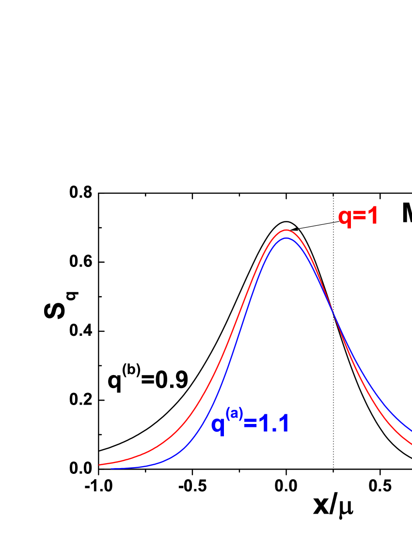
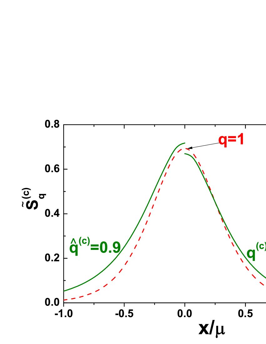
Figure 1: (Color online) Schematic view of $S_{q}=\tilde{S}^{(R=a,b)}_{q}$ defined by Eqs. (57) and (58) (left panel) and $S_{q}^{(c)}=\tilde{S}^{(R=c)}$ defined by Eq. (59) (right panel), all presented as a function of the scaled variable $x/\mu$. The respective values of $q$ used are shown. All these results are compared with the extensive case of $q=1$ (blue curves). Calculations were performed assuming $M_{qi}=0$, $T=60$ MeV and $\mu=322$ MeV. The meaning of $q$ and $\hat{q}$ on the right panel corresponds to definition of $\tilde{q}$ presented in Eq. (39).

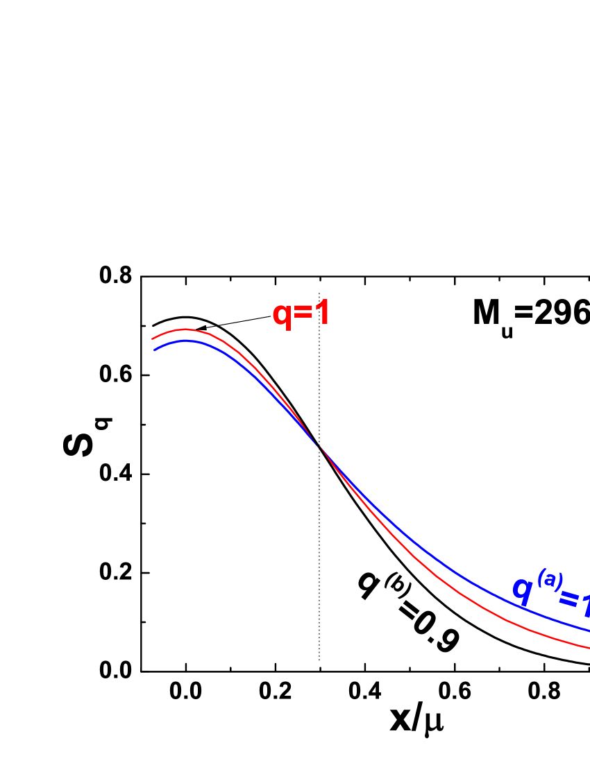
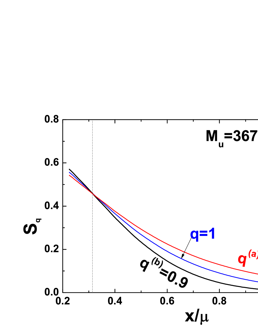
Figure 2: (Color online) The same as in the left panel of Fig. 1 but for different masses $M_{u}$.

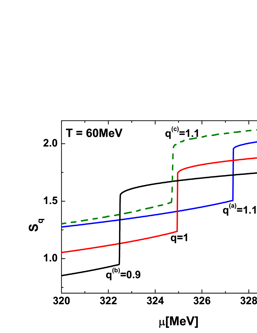
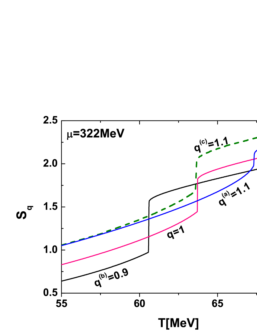
Figure 3: (Color online) Entropy as a function of the chemical potential (left panel) and temperature (right panel) calculated for different values of $q$ corresponding to different realizations of the $q$-NJL model and compared with the BG case of $q=1$.

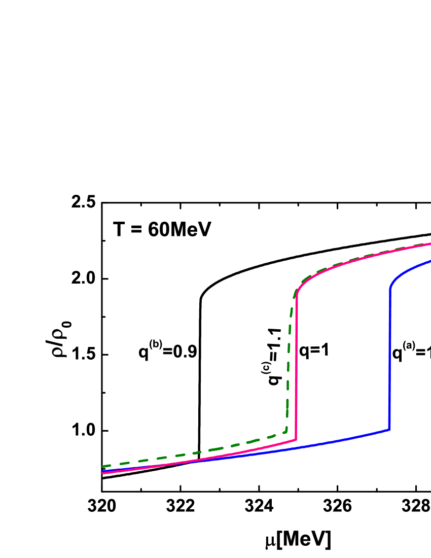
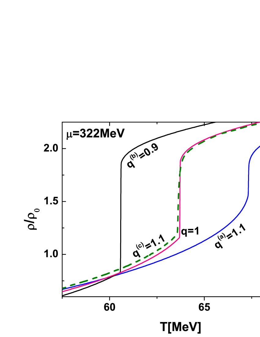
Figure 4: (Color online) Compression $\rho/\rho_{0}$ as a function of the chemical potential (left panel) and the pressure (right panel) for different values of $q$ corresponding to different realizations of the $q$-NJL model and compared with the BG case of $q=1$.

4.3 Results for entropy, pressure and compression

After the preparatory explanations in the previous section we present now results for entropy $S$ (Fig. 3), pressure $P$ (Fig. 5) and density $\rho$ (Fig. 4). Calculations were performed for $T=60$ MeV and $\mu=322$ MeV, for different values of $q$ corresponding to different realizations of the $q$-NJL model and compared with the BG case of $q=1$. This choice of values of $T$ and $\mu$ is dictated by the fact that, as can be seen in Table 1, they are near to the critical values corresponding to the values of nonextensive parameter $q$ considered here. For this choice the critical effects displayed in the presented figures are most visible. Chemical potentials and temperatures at which one observes rapid changes of entropy (Fig. 3) and small jumps in the pressure (Fig. 5), correspond to regions of phase transition in which the density of fermions changes rapidly, approximately from $\rho_{0}$ to $2\rho_{0}$, as seen in Fig. 4.

The general characteristic feature of these results is the horizontal shift of the phase transition point and of all curves for entropy $S$ and density $\rho/\rho_{0}$, when calculated for a fixed value of temperature $T=60$ MeV, towards smaller values of $\mu$ for $q<1$ (case $(b)$) and towards greater values of $\mu$ for $q^{(a)}=1.1$ (case$(a)$). For densities below and above well separated critical points all curves converge. At the same time $S_{q=1.1}^{(a)}>S_{q=1}$, i.e. it exceeds the BG entropy, whereas $S^{(b)}_{q=0.9}$ is smaller than the BG entropy. In case $(c)$, in which $q=1.1$ above the Fermi surface and changes to $\hat{q}=2-q=0.9$ below it, one observes more complicated behavior. Whereas the transition point remains nearly the same as in the BG case, the value of entropy $S_{q}^{(c)}$ exceeds considerably that of $S^{(a)}_{q=1.1}$ above the phase transition point and practically coincides with it below this point. This behavior reflects that of $\tilde{S}_{q}^{(R=a,b,c)}$ shown in Figs. 1 and 2 (one must remember that $M_{u}$ is a minimum above the phase transition point and a maximum below it).

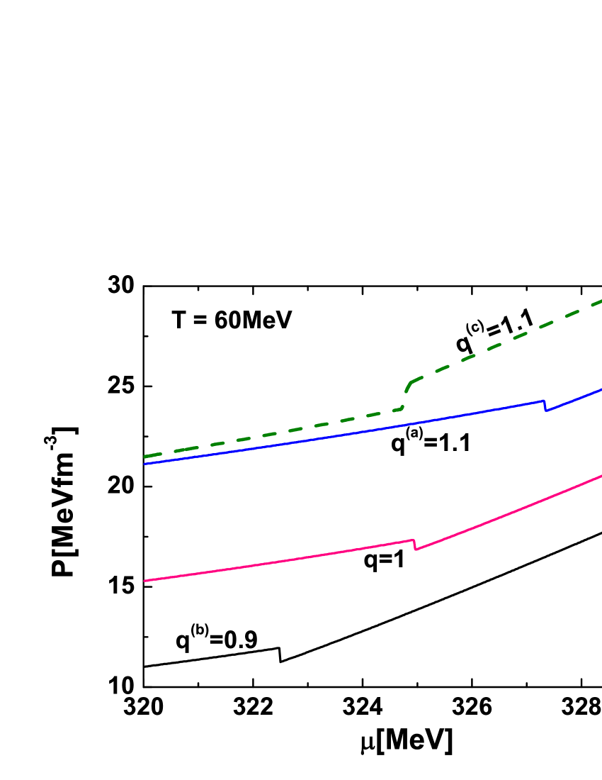
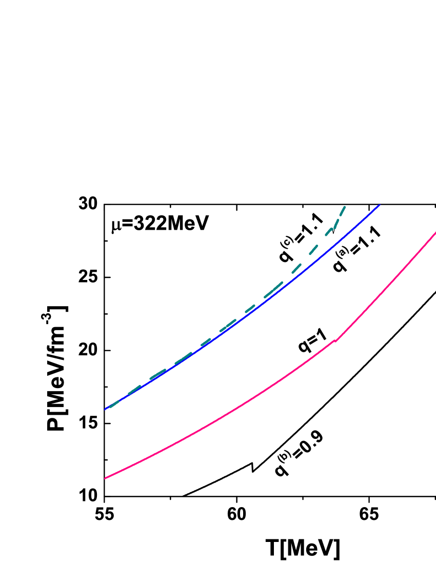
Figure 5: (Color online) Pressure as a function of the chemical potential (left panel) and pressure (right panel) for different values of $q$ corresponding to different realizations of the $q$-NJL model and compared with the BG case of $q=1$.

Behavior of pressure $P$ is shown in Fig. 5. Its increase as a function of $\mu$ is dictated by the derivative $\rho=\partial P/\partial\mu|_{T}$ (and depends on the behavior of $\rho$ presented in Figure 4), whereas its increase as a function of $T$ is given by the derivative $s=\partial P/\partial T|_{\mu}$ (and is given by the behavior of $S$ in Fig. 3). Looking at Figs. 3-4 from this perspective, we observe generally that both the entropy and density are lower below the phase transition than after it. The corresponding increase of pressure before the phase transition is therefore weaker than in unconfined phase. This behavior is more pronounced when considered as a function of temperature $T$ rather than as a function of chemical potential $\mu$. Note that because, as seen in Fig. 4, densities are very similar for different realizations of the $q$-NJL model, the resulting pressure curves as a function of chemical potential are almost parallel. Because entropies differ much more strongly the dependence on temperature is more divergent for different realizations of the $q$-NJL model.

4.4 In the vicinity of the phase transition point

We shall present now the behavior in the vicinity of critical values of $T$ and $\mu$ and present results for pressure, compression, heat capacity $C_{\mu}$, baryon number susceptibility $\chi$ and the phase diagram.

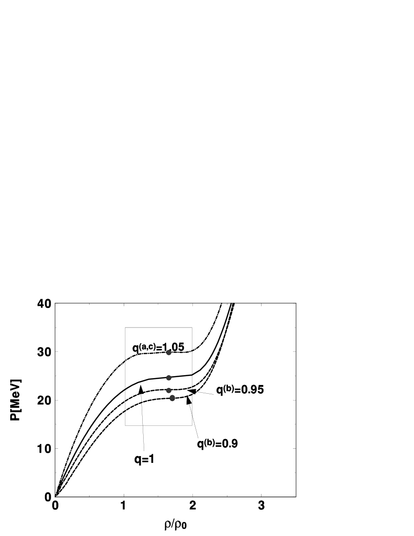
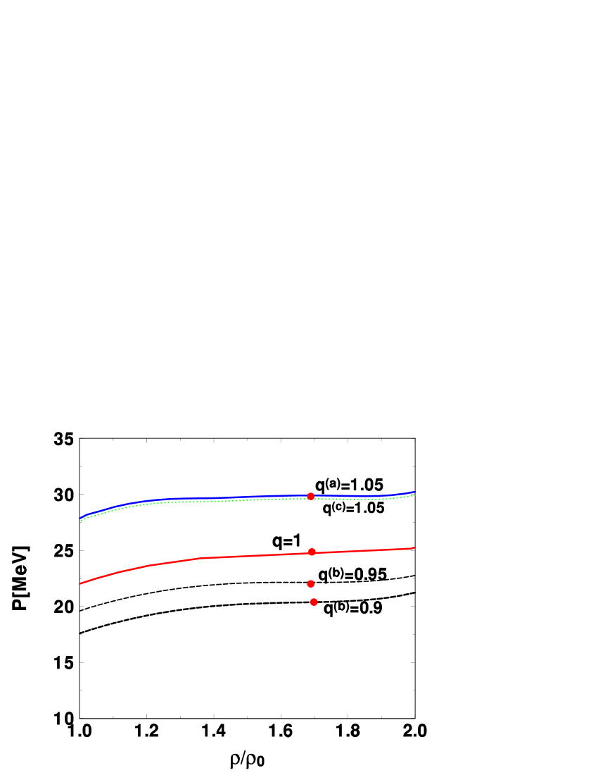
Figure 6: (Color online) The pressure at critical temperature $T_{cr}$ as a function of compression $\rho/\rho_{0}$ calculated for different values of $q$ corresponding to different realizations of the $q$-NJL model and compared with the BG case of $q=1$ (the area marked on the upper panel is shown in detail in the lower panel). The dots indicate the positions of the inflection points for which the first derivative of pressure by compression vanishes.

Fig. 6 presents the pressure at the critical temperature $T_{cr}$ (critical isotherms) for the corresponding critical values of the chemical potential, $\mu_{cr}$, as a function of compression $\rho/\rho_{0}$. The values of $T_{cr}$ and $\mu_{cr}$ determine the critical values of pressure and density corresponding to the inflection points for which the first derivative of pressure by compression vanishes. They are listed in Table 1. Remarkably, in all these cases the critical density remains practically the same. The other interesting observation is that the results for choice $(a)$ essentially coincide with those for choice $(c)$. For $q>1$, we observe an increase of the pressure $P$ (corresponding to a similar increase of the entropy in this case observed in Fig. 3). This increase may simulate some additional repulsion between massive quarks constituting nucleons at short distances (which is present in quark-meson coupling models based on the mean field approach QMC ; QMC1 ). On the contrary, for $q<1$ we observe a decrease of the critical pressure (corresponding to a decrease of entropy, seen in Fig. 3). This could simulate confinement of quarks in nucleons which introduces restrictions in phase space by changing their Fermi motion.

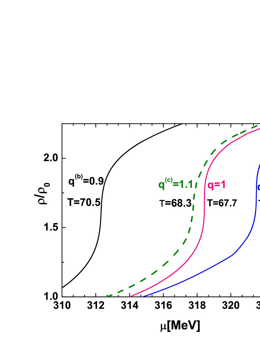
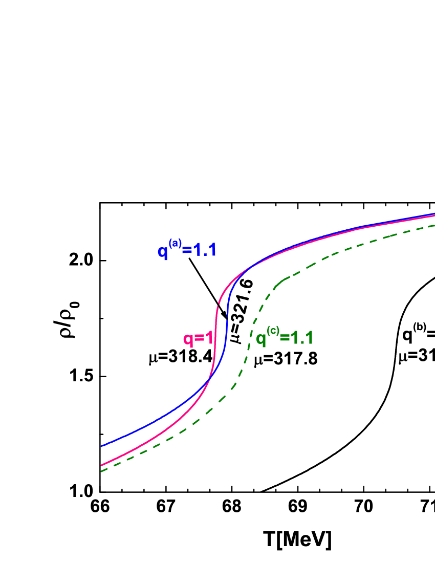
Figure 7: (Color online) Compression $\rho/\rho_{0}$ as a function of chemical potential (left panel) and temperature (right panel) calculated in the vicinity of the phase transition for different values of $q$ corresponding to different realizations of the $q$-NJL model and compared with the BG case of $q=1$.

Table 1: The values of the critical temperature, $T_{cr}$, and the critical chemical potential, $\mu_{cr}$, for different realizations of the $q$-NJL model.

	$T_{cr}$ [MeV]	$\mu_{cr}$ [MeV]
$q^{(a)}=1.1$	$67.9$	$321.6$
$q^{(b)}=0.9$	$70.5$	$312.3$
$q^{(c)}=1.1$	$68.3$	$317.8$
$q=1$	$67.7$	$318.4$

In Fig. 7 we present compression as a function of chemical potential $\mu$ and temperature $T$ but now, unlike in Fig. 4, calculated in the vicinity of the phase transition point (the corresponding values of $T_{cr}$ and $\mu_{cr}$ are given in Table 1). Because both $T$ and $\mu$ now change their values, the observed behavior of $\rho/\rho_{0}$ is very different from the previously one. It is dictated by the fact that, as seen in Table 1, in our $q$-NJL model we have $T_{cr}^{(q=1)}<T_{cr}^{(a)}<T^{(c)}_{cr}<T^{(b)}_{cr}$ and $\mu^{(a)}_{cr}>\mu^{(q=1)}_{cr}>\mu^{(c)}_{cr}>\mu^{(b)}_{cr}$.

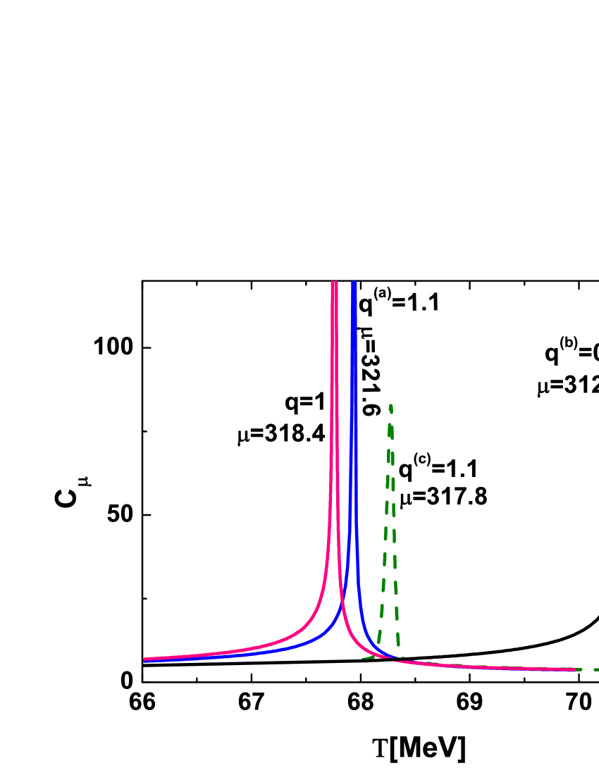
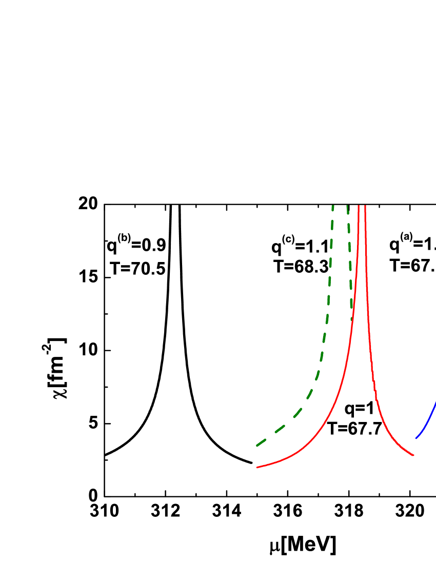
Figure 8: (Color online) Left panel: Heat capacity as a function of temperature calculated in the vicinity of the phase transition point for different values of $q$ corresponding to different realizations of the $q$-NJL model and compared with the BG case of $q=1$. The respective values of chemical potential used are indicated. Right panel: Susceptibility as a function of chemical potential calculated in the vicinity of the phase transition point, and for different values of $q$ corresponding to different realizations of the $q$-NJL model and compared with the BG case of $q=1$. The respective values of the temperatures are indicated.

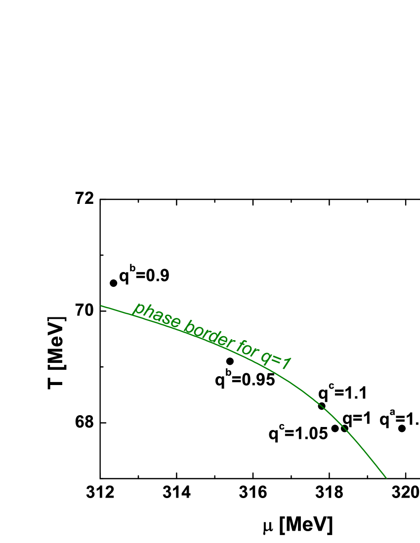
Figure 9: (Color online) Phase diagram in the $q$-NJL model in the $T-\mu$ plane for different values of $q$ corresponding to different realizations of the $q$-NJL model and compared with the BG case of $q=1$. The left panel shows a general view where, for the scale used, all curves essentially coincide. The right panel shows an enlarged region near the critical point (CEP).

In Fig. 8 we present our results for, respectively, heat capacity (not calculated before in RWJPG ; RWConf ; RWConf1 ) and baryon susceptibilities. Both were calculated for the critical values of the chemical potential and temperature listed in Table 1. As one can see in left panel of Fig. 8, for $q^{(b)}=0.9$ the critical point is shifted towards higher values of temperature, $T_{crit}=70.5$ MeV. In this region we also observe that the chemical potential at the critical point is lower, $\mu_{crit}=312$ MeV, in comparison to its extensive value for $q=1$, $\mu_{crit}=318.4$ MeV. As a result, the critical points for $q^{(b)}<1$ lie very close the extensive phase border, as seen in Fig. 9. For $q^{(a)}=1.1$ (and partially also for $q^{(c)}=1.1$) the critical temperature $T_{crit}$ remains very near its extensive value for $q=1$, $T_{crit}=70.5$ MeV, but the critical chemical potential is shifted towards larger values, see Fig. 9 and Fig. 8 (right panel).

As seen in Fig. 7 and Fig. 9 the results for $T_{crit}$ are for choice $(c)$ are very near to those for choice $(a)$ whereas the results for $\mu_{crit}$ are for choice $(c)$ very near to the results for $q=1$. Consequently, whereas the critical coordinates in cases $(a)$ and $(b)$ depart from the extensive phase border line in Fig. 9, the critical coordinates for choice $(c)$ are very close to the extensive limit of $q=1$. This reflects the fact that in choice $(c)$ we use at the same time both $q>1$ and $q<1$ (depending on the region of phase space actually considered) minimizing therefore the departure from the extensive dynamics.

The results presented in Figs. 9, 6 and in the right panel of 8 can be compared with the corresponding results obtained in our previous version of the $q$-NJL model (with Figs. 4 and 8 in RWJPG , with Fig. 1 in our first paper in RWConf ; RWConf1 and with Figs. 1-3 and 5 in our second paper there). This allows us to estimate what kind and how big are the changes introduced by proper treatment of thermodynamical consistency. Quantitatively the corresponding results look similar, there are differences in what concerns sensitivity to deviation from extensivity leading to quantitatively similar effects: the previous $|q-1|\sim 0.02$ should be confronted with the present $\sim 0.1$. The detailed shape of the phase diagram or detailed shapes of some distributions are also different, although, not dramatically so. The most visible, but still rather small, difference concerns the case with $q<1$. For example, the previously presented $\chi$ was much smaller and broader than the corresponding result for $q>1$, at present they are comparable in shape and height (compare right panel of our Fig.8 and Fig.5 in the second paper of RWConf ; RWConf1 ). Also, the sensitivity to changes in $q$ in the vicinity of the phase transition point seems to be reversed. Comparing our Fig. 6 and Fig. 1 in RWConf ; RWConf1 one notices greater changes for $q<1$ than for $q>1$ observed before, and the reverse behavior is seen in the present results. This is so far the most visible difference resulting from the fact that now $q<1$ is described entirely by case $(b)$ only. The most similar to what was used before in RWJPG ; RWConf ; RWConf1 is case $(c)$, already explained in detail.

5 Summary and conclusions

The results presented above confirm the previously reached conclusions concerning the applicability and usefulness of the nonextensive approach as one of the possible extensions of the original mean field theory, extending considerably the range of its applicability. However, this time they were obtained in compliance with all the conditions that must be satisfied when implementing a nonextensive approach to systems with particles and antiparticles and a nonzero chemical potential (which were so far overlooked) JR . Out of three possible formulations investigated in detail in sections (3.2), (3.3) and (3.4) (and denoted by $(a)$, $(b)$ and $(c)$, respectively), the most consistent, in our opinion, is approach $(a)$ for $q>1$ or $(b)$ for $q<1$.

Approach $(c)$ requires more attention. There are two features which should be commented on. The first is that our results in Fig. 3 show that the jump in entropy $S^{(c)}$ (for $q^{(c)}=1.1$) occurs almost at the same point as that for the extensive case of $q=1$. This is because in case $(c)$ we have, in fact, two values of the nonextensive parameter: $q$ above the Fermi surface and $2-q$ below it (equal, correspondingly, to $1.1$ and $0.9$ in our case). As can be seen in Fig. 3, the corresponding shifts for $q>1$ and $q<1$ are in opposite directions. Therefore, we see here a kind of cancellation of two opposite effects. The second feature, visible in Fig. 1 (lower panel) is the jump in entropy on the Fermi surface (which occurs because of the above mentioned change in nonextensivity parameter there). However, in nuclear matter we do not observe a sharp change of entropy on the Fermi surface (i.e. for $x=0$) in the extensive situation of $q=1$ which could possibly be modeled by introducing a nonextensive environment with $q\neq 1$. The transition from the bound state to the continuum is always gradual Pairing ; Pairing1 .

As discussed before in Section 3.4, case $(c)$ was proposed in order to avoid Tsallis’ cut-offs introduced in cases $(a)$ and $(b)$ (cf. Eq. (27)). These cut-offs result in the artificial fixing of the respective occupation numbers in some regions of phase space to be equal either to unity (particles) or zero (antiparticles) (cf. Eqs. (26) and (27) or (28)-(30)). They are therefore regarded as unjustified additional ingredients of the $q$-NJL model. However, it seems that the price of introducing case $(c)$, which eliminates the need for such restrictions, is too high to be acceptable for the reasons mentioned above. The cut-off of part of the phase space seems to be more reasonable in this respect. To add to these arguments, note that when crossing the Fermi level the quark mass does not change, whereas it changes in the phase transition.

In our revisited non-extensive, but thermodynamically consistent, $q$-NJL model, we can perform calculations for both $q<1$ and $q>1$ statistical effects. Some comments regarding their possible roles are therefore necessary. Note first that the main approximation in the NJL mean field theory description concerns the phase with condensates, where the quarks are not confined but rather become less massive approaching the phase transition region and practically massless when crossing it (in the same way as in our previous version of the $q$-NJL model, cf. Fig. 1 in RWJPG ). In the usual NJL mean field model confinement is not present; it can be introduced by adding a dynamical gluon field, for example, in the form of a Polyakov loop PLoop ; PLoop1 ; PLoop2 . On the other hand, confinement of quarks in nucleons introduces restrictions in the allowed phase space by changing their Fermi motion and decreasing the chemical potential. It increases quark arrangement in nuclear matter and, consequently, decreases the entropy and effectively also the pressure between such composite objects as nucleons. Such effects are visible in our $q$-NJL model with $q<1$. This means that for the phase with vacuum condensates the $q<1$ description could adequately describe the correlations which are responsible for the changes in the arrangement of quarks and therefore model, to some extent, the effect of confinement. These correlations will survive even in the unconfined phase (i.e. entropy there remains lower than in other cases). Also, as seen in Table 1, the critical temperature for $q<1$ is higher ($T^{(b)}_{cr}=70.5$ MeV), whereas the corresponding entropy becomes smaller. This is understandable because at lower entropy we need larger temperature to convey the same amount of energy.

For the case of $q>1$ (case $(a)$) the average single particle energy (chemical potential) is shifted towards higher values and the entropy and pressure are also higher, increasing the Fermi energy. The critical temperature (both for case $(a)$ and case $(c)$) remains practically the same as for the extensive case with $q=1$. The increase of pressure may simulate some additional repulsion (at short distances) between massive quarks constituting nucleons (see, for example, the quark-meson coupling models QMC ; QMC1 ). This means that, effectively, $q>1$ could be regarded as emerging from the increasing nonstatistical fluctuations found in the decay of dense fireballs produced in heavy ion collisions and in other multiparticle production experiments multipart ; multiparta ; qMB ; multipart1 ; multipart1a ; multipartB ; mpo ; mpo1 ; mpo2 ; mpo3 ; mpo4 ; mpo5 ; CW ; CWa .

Summarizing, the nonextensive description accounts (in a phenomenological way) for all situations in which one expects some dynamical correlations in the quark-antiquark system considered in our $q$-NJL model. It must be stressed that the nonextensive approach is not a substitute for any part of the interaction described already by the lagrangian of the NJL model, cf. Eq. (4). It rather provides a different environment which can have some dynamical effects, so far undisclosed but simply parameterized by nonextensivity $q$. From this perspective case $(b)$ with $q<1$, which has lower entropy, seems to be more suitable to describe the nonextensive mechanism in the Equation of State (EoS) of dense hadronic matter in a restricted phase space, like, for example, in (proto)neutron stars. Respectively, the case $(a)$, with $q>1$ and with higher entropy, is more suitable for situations in which one expects dynamical fluctuations, for example to describe heavy ion collision where dense nuclear matter is created out of equilibrium and quickly decays into hadrons. Our work therefore presents arguments that the critical properties of nuclear matter in two different environments can be different, although the phase transition occurs at the same density or compression. The critical temperature is higher for nuclear matter created in (proto)neutron stars but the critical value of the chemical potential will be bigger for nuclear matter created in heavy ion collisions

We conclude with two remarks. First: our approach should not be confounded with the similar in spirit approach based on quantum algebras (or on the so called $q$-deformed algebras) which was used to formulate a $q$-deformed NJL model QA . Their common feature is the use of some suitable deformation of the mean field NJL model (based on nonextensive statistical mechanics in our case and on quantum algebras in QA ), which may account for intrinsic correlations and fluctuations that go beyond the mean field formulation and, in a certain limit, approach the more realistic lattice calculations. Second: there exists another, potentially very interesting, approach to nonextensivity, based on the so called Kaniadakis entropy KanS ; KanS1 ; KanS2 . In QCD_kappa it was used to study the formation of the quark-gluon plasma formation (and compared with nonextensive approach) whereas in Walecka_kappa it was used to investigate the relativistic nuclear EoS in the context of the Walecka quantum hadrodynamics theory.

Acknowledgments

The research of GW was supported in part by the National Science Center (NCN) under contract Nr 2013 /08/M /ST2 /00598 (Polish agency). We would like to thank warmly Dr Nicholas Keeley for reading the manuscript.

References

- (1) Y. Nambu and G. Jona-Lasinio, Phys. Rev. 122, 345 (1961).
- (2) Y. Nambu and G. Jona-Lasinio, Phys. Rev. 124, 246 (1961).
- (3) S. P. Klevansky, Rev. Mod. Phys. 64, 649 (1992).
- (4) P. Rehberg, S. P. Klevansky and J. Hüfner, Phys. Rev. C 53, 410 (1996).
- (5) T. Hatsuda and T. Kunihiro, Phys. Rep. 247, 221 (1994).
- (6) V. Bernard, U-G. Meissner and I. Zahed, Phys. Rev. D 36, 819 (1987).
- (7) M. Buballa, Phys. Rep. 407, 205 (2005).
- (8) P. Costa, M. C. Ruivo and C.A. de Sousa, Phys. Rev. D 77, 096001 (2008).
- (9) P. Costa, M. C. Ruivo, C.A. de Sousa and Yu. L. Kalinovsky, Phys. Rev. C 70, 025204 (2004).
- (10) J. Rożynek and G. Wilk, J. Phys. G 36, 125108 (2009).
- (11) J. Rożynek and G. Wilk, Acta Phys. Polon. B 41, 351 (2010.
- (12) J. Rożynek and G. Wilk, EPJ Web of Conferences 13, 05002 (2011).
- (13) J. D. Walecka, Ann. Phys. 83, 491 (1974).
- (14) S. A. Chin and J. D. Walecka, Phys. Lett. B 52, 1074 (1974).
- (15) B. D. Serot and J. D. Walecka, Adv. Nucl. Phys. 16, 1 (1986).
- (16) F. I. M. Pereira, R. Silva and J. S. Alcaniz, Phys. Rev. C 76, 015201 (2007).
- (17) F. I. M. Pereira, R. Silva and J. S. Alcaniz, Phys. Let. A 373, 4214 (2009).
- (18) P. Costa, C. A. de Sousa, M. R. Ruivo and H. Hansen, Europhys. Lett. 86, 31001 (2009).
- (19) A. Drago, A. Lavagno and P. Quarati, Physica A 344, 472 (2004).
- (20) A. Lavagno, P. Quarati and A.M. Scarfone, Braz. J. Phys. 39, 457 (2009).
- (21) A. Lavagno, D. Pigato and P. Quarati, J. Phys. G 37, 115102 (2010).
- (22) G. Gervino, A. Lavagno and D. Pigato, Cent. Eur. J. Phys. 10, 594 (2012).
- (23) A. Lavagno and D. Pigato, J. Phys. G 39, 125106 (2012).
- (24) T. S. Biró and G. Purcsel, Centr. Eur. J. Phys. 7, 395 (2009).
- (25) T. S. Biró, G. Purcsel and K. Ürmösy, Eur. Phys. J. A 40, 325 (2009).
- (26) C. Tsallis, J. Stat. Phys. 52, 479 (1988); Eur. Phys. J. A 40, 257 (2009).
- (27) C. Tsallis, Contemporary Physics, 55, 179 (2014).
- (28) C. Tsallis, Acta Phys. Pol. B 46 (2015) 1089.
- (29) C. Tsallis, Introduction to Nonextensive Statistical Mechanics (Springer, Berlin, 2009). For an updated bibliography on this subject, see http://tsallis.cat.cbpf.br/biblio.htm.
- (30) T. Osada and G. Wilk, Phys. Rev. C 77, 044903 (2008) [erratum: Phys. Rev. C 78, 069903(E) (2008)].
- (31) T. Osada and G. Wilk, Centr. Eur. J. Phys. 7, 432 (2009).
- (32) G. Wilk and Z. Włodarczyk, Eur. Phys. J. A 40, 299 (2009).
- (33) G. Wilk and Z. Włodarczyk, Eur. Phys. J. A 48, 161 (2012).
- (34) M. Biyajima, T. Mizoguchi, N. Nakajima, N. Suzuki and G. Wilk, Eur. Phys. J. C 48, 597 (2006).
- (35) G. Wilk and Z. Włodarczyk, Eur. Phys. J. A 48, 161 (2012).
- (36) G. Wilk and Z. Włodarczyk, Cent. Eur. J. Phys. 10 568 (2012).
- (37) T. S. Biró, G. G. Barnaföldi and P. Ván, Eur. Phys. J. A 49, 110 (2013).
- (38) C. Beck, Physica A 286, 164 (2000).
- (39) W. M. Alberico and A. Lavagno, Eur. Phys. J. A 40, 313 (2009).
- (40) B. De, Eur. Phys. J. A 50, 70 (2014).
- (41) B. De, Eur. Phys. J. A 50, 138 (2014).
- (42) M. Rybczyński and Z. Włodarczyk, Eur. Phys. J. C 74, 2785 (2014).
- (43) T. Wibig, Eur. Phys. J. C 74, 2966 (2014).
- (44) M. D. Azmi and J. Cleymans, J. Phys. G 41, 065001 (2014).
- (45) L. Marques, J. Cleymans and A. Deppman, Phys. Rev. D 91, 054025 (2015).
- (46) T. S. Biró and G. Purcsel, Phys. Rev. Lett. 95, 162302 (2005).
- (47) T. S. Biró and G. Purcsel, Phys. Lett. A 372, 1147 (2008).
- (48) T. S. Biró, Europhys. Lett. 84,56003 (2008).
- (49) T. S. Biró and A. Peshier, Phys. Lett. B 632, 247 (2006).
- (50) T. S. Biró, K. Ürmösy and Z. Schram, J. Phys. G 37, 094027 (2010).
- (51) T. S. Biró and Z. Schram, Pisma ECzAJA 8, C20 (2011).
- (52) T. S. Biró, K. Urmössy and Z. Schram, J. Phys. G 37, 094027 (2010).
- (53) T. S. Biró and Z. Schram, Polyakov Loop Behavior in Non-Extensive SU(2) Lattice Gauge Theory, arXiv:1105.1931[hep-lat].
- (54) T. S. Biró and Z. Schram, EPJ Web of Conferences 13, 5004 (2011).
- (55) G. Wilk and Z. Włodarczyk, AIP Conf. Proc. 1558, 893 (2013).
- (56) G. Wilk and Z. Włodarczyk, Entropy 17, 384 (2015).
- (57) G. Wilk and Z. Włodarczyk, Chaos Solitons and Fractals 81, 487 (2015).
- (58) G. Wilk and Z. Włodarczyk, Acta Phys. Pol. B 46, 1103 (2015).
- (59) C.-Y. Wong and G. Wilk, Phys. Rev. D 87, 114007 (2013).
- (60) C.-Y. Wong, G. Wilk, L. J. L. Cirto and C. Tsallis, Phys. Rev. D 91, 114027 (2015).
- (61) O. J. E. Maroney, Phys. Rev E 80, 061141 (2009);
- (62) T. S. Biró, K. Ürmössy and Z. Schram, J. Phys. G 37, 094027 (2010).
- (63) T. S. Biró and P. Vań, Phys. Rev. E 83, 061147 (2011).
- (64) T. S. Biró and Z. Schram, Eur. Phys. J. Web Conf. 13, 05004 (2011).
- (65) T. S. Biró, Is there a Temperature? Conceptual Challenges at High Energy, Acceleration and Complexity (Springer, New York Dordrecht Heidelberg London, 2011).
- (66) P. Ván, G. G. Barnaföldi, T. S. Biró and K. Ürmössy, J. Phys. Conf. Ser. 394, 012002 (2012).
- (67) J. Randrup, Phys. Rev. C 79, 054911 (2009).
- (68) L. F. Palhares, E. S. Fraga and T. Kodama, J. Phys. G 37, 094031 (2010).
- (69) V. V. Skokov and D. N. Voskresensky, JETP Lett. 90, 223 (2009).
- (70) V. V. Skokov and D. N. Voskresensky, Nucl. Phys. A 828, 401 (2009).
- (71) P. M. Lo, J. Phys. Conf. Ser. 503, 012034 (2014).
- (72) P. M. Lo, Acta Phys. Polon. B (proc. Suppl.) 7, 99 (2014).
- (73) K. Fukushima, Phys. Rev. D 77, 114028 (2008).
- (74) J. Rożynek, Physica A 440, 27 (2015).
- (75) A. R. Plastino, A. Plastino, H. G. Miller and H. Uys, Astroph. and Space Sci. 290, 275 2004.
- (76) A. M. Teweldeberhan, A. R. Plastino and H. C. Miller, Phys. Lett. A 343, 71 (2005).
- (77) A. M. Teweldeberhan, H. G. Miller and R. Tegen, Int. J. Mod. Phys. E 12, 395 (2003).
- (78) J. M. Conroy, H. G. Miller and A. R. Plastino, Phys. Lett. A 374, 4581 (2010).
- (79) J. Cleymans and D. Worku, J. Phys. G 39, 025006 (2012).
- (80) J. Cleymans and D. Worku, Eur. Phys. J. A 48, 160 (2012).
- (81) A. Lavagno, D. Pigato, Physica A 392, 5164 (2013).
- (82) A. Lavagno, D. Pigato, Eur. Phys. J. A 47, 52 (2011).
- (83) A. P. Santos, F. I. M. Pereira, R. Silva and J. S. Alcaniz, J. Phys. G 41, 055105 (2014).
- (84) E. Megias, D. P. Menezes and A. Deppman, Physica A 421, 15 (2015).
- (85) A. Deppman, J. Phys. G 41, 055108 (2014).
- (86) A. Deppman, Physica A 391, 6380 (2012) [erratum: Physica A 400, 207 (2014)].
- (87) I. Sena and A. Deppman, Eur. Phys. J. A 49, 17 (2013).
- (88) I. Sena and A. Deppman, AIP Conf. Proc. 1520, 172 (2013).
- (89) L. Marques, E. Andrade-II and A. Deppman, Phys. Rev. D 87, 114022 (2013).
- (90) E. Meg as, D.P. Menezes and A. Deppman, EPJ Web of Conferences 80, 00040 (2014).
- (91) A. Deppman, E. Meias and D. P. Menezes, J. Phys. Conf. Ser. 607, 012007 (2015).
- (92) G. Wilk and Z. Włodarczyk, Phys. Rev. Lett. 84, 2770 (2000).
- (93) G. Wilk and Z. Włodarczyk, Chaos, Solitons, Fractals 13, 581 (2002).
- (94) T. S. Biró and A. Jakovác, Phys. Rev. Lett. 94, 132302 (2005).
- (95) T. Kodama, H.-T. Elze, C.E. Aguiar, and T. Koide, 2005 Europhys. Lett. 70, 439 (2005).
- (96) T. Kodama, and T. Koide, Eur. Phys. J. A 40, 289 (2009).
- (97) V. Garcia-Morales, and J. Pellicer, Physica A 361, 161 (2006).
- (98) J. N. Kapur and H. K. Kesavan, 1992, Entropy Optimization Principles with Applications, Academic Press (1992), San Diego.
- (99) A. Sommerfeld, 1993, Thermodynamics and Statistical Mechanics, Academic Press (1993), New York.
- (100) A. Plastino and A.R. Plastino, Phys. Lett. A 226, 257 (1997).
- (101) T. Yamano, Eur. Phys. J. B 18, 103, (2000).
- (102) T. Herbst, M. Mitter, J. M. Pawlowski, B-J. Schaefer and R. Stiele, Phys. Lett. B 731, 248 (2014).
- (103) J. Arrington, D.W. Hibotham, G. Rosner and M. Sargsian, Prog. Nucl. Part. Phys. 67, 898 (2012).
- (104) T. S. Biró, K. M. Shen and B. W. Zhang, Physica A 428, 410 (2015).
- (105) D.P. Menezes, A. Deppman, E. Megias and L.B. Castro, Eur. Phys. J. A 51, 155 (2015).
- (106) K. Saito and A.W. Thomas, Phys. Lett. B 327, 9 (1994).
- (107) P. A. Guichon, Phys. Lett. B 200 363(1988).
- (108) K.-I. Aoki, and M. Yamada, Int. J. Mod. Phys. A 30, 1550180 (2015).
- (109) J. Sólyom, Fundamentals of the Physics of Solids, Vol. 3 - Normal, Broken-Symmetry, and Correlated Systems, Springer-Verlag Berlin Heidelberg (2010).
- (110) H. Hoffman, The Physics of Warm Nuclei, Oxford University Press, Oxford, 2008, pp. 79 84.
- (111) M. Fellah, N.H. Allal, M. Belabbas, M.R. Oudih, N. Benhamouda, Phys. Rev. C 76, 047306 (2007).
- (112) P.B. Demorest, T. Pennucci, S. M. Ransom, M.S.E. Roberts and J.W.T. Hessels, Nature 467, 7319 (2010).
- (113) J. Antoniadis et al., Science 340, 6131 (2013).
- (114) S. S. Avancini, J.R. Marinelli, D.P. Menezes, and M.M. Watanabe de Moraes, Phys. Lett. B 507, 129 (2001).
- (115) G. Kaniadakis, Eur. Phys. J. A 40, 275 (2009).
- (116) G. Kaniadakis, Eur. Phys. J. B 70, 3 (2009).
- (117) G. Kaniadakis, Eur. Phys. Lett. 92, 35002 (2010).
- (118) A.M . Teweldeberhan, H.G. Miller and R. Tegen, Int. J. Mod. Phys. E 12, 669 (2003).
- (119) F.I.M. Pereira, R. Silva and J.S. Alcaniz, Nucl. Phys. A 828, 136 (2009).