Probing Wilson loops in $\mathcal{N}=4$ Chern–Simons–matter theories at weak coupling

Abstract

For three–dimensional ${\cal N}=4$ super Chern–Simons–matter theories associated to necklace quivers $U(N_{0})\times U(N_{1})\times\cdots U(N_{2r-1})$, we study at quantum level the two kinds of 1/2 BPS Wilson loop operators recently introduced in arXiv:1506.07614. We perform a two–loop evaluation and find the same result for the two kinds of operators, so moving to higher loops a possible quantum uplift of the classical degeneracy. We also compute the 1/4 BPS bosonic Wilson loop and discuss the quantum version of the cohomological equivalence between fermionic and bosonic Wilson loops. We compare the perturbative result with the Matrix Model prediction and find perfect matching, after identification and remotion of a suitable framing factor. Finally, we discuss the potential appearance of three–loop contributions that might break the classical degeneracy and briefly analyse possible implications on the BPS nature of these operators.
PACS numbers: 11.25.Hf, 11.30.Pb, 11.15.Yc, 11.10.Kk

I Introduction

One of the most interesting classes of observables in supersymmetric gauge theories is constitued by BPS Wilson loops Erickson:2000af ; Drukker:2000rr . They provide an exciting arena where exact computations can be performed through localization techniques Pestun:2007rz , so interpolating non-trivially between weak and strong coupling regimes.

The first and most famous example is the 1/2 BPS circular Wilson loop, originally constructed in ${\cal N}=4$ super Yang-Mills theory. It is calculated by a simple Gaussian matrix model and reproduced at strong coupling through the AdS/CFT correspondence Erickson:2000af ; Drukker:2000rr . The original proposal has been generalized to less supersymmetric loops Drukker:2007qr and in theories with ${\cal N}=2$ supersymmetry Pestun:2007rz . In all these constructions the key point is to improve the holonomy of the gauge connection by coupling some of the scalar fields to the appropriate contours. The resulting operators are BPS and their expectation values can be computed by adding a suitable Q-exact term to the classical action, so that the relevant path-integral is semiclassically exact Pestun:2007rz .

In three dimensions the story is a little bit different. ${\cal N}=2$ Chern-Simons theories still possess circular 1/2 BPS Wilson loops obtained through scalar couplings, which are calculated by localization techniques Kapustin:2009kz . Going to more supersymmetric theories, as the ${\cal N}=6$ ABJ(M) model, the construction of 1/2 BPS operators has to be refined Drukker:2009hy (see also Cardinali for a generalization to other contours). In fact, scalar couplings only provide 1/6 BPS Wilson loops and fermionic couplings have to be invoked to enhance supersymmetry. More surprisingly, 1/2 BPS Wilson loops in ABJ(M) theory are seen equivalent to a linear combination of 1/6 BPS ones Drukker:2009hy ; Drukker:2010nc . In fact, they belong to the same cohomology class of the localizing supercharge and thus, up to framing anomalies, they are the same observable at quantum level. This phenomenon is a three-dimensional novelty, that has been checked concretely in perturbation theory Bianchi:2013rma ; Griguolo:2013sma and certainly needs a more profound investigation. Recently, the construction of 1/2 BPS Wilson loops has been presented Ouyang:2015qma ; Cooke:2015ila in ${\cal N}=4$ quiver Chern-Simons theories Gaiotto:2008sd ; Hosomichi:2008jd . In the case of circular and linear quivers with non-vanishing CS levels, two apparently independent 1/2 BPS circular loops emerge, which share the same supersymmetry and belong to the same cohomology class of the familiar bosonic 1/4 Wilson loop operator. These properties have been derived at classical level and should be checked against truly quantum computations, where divergences and/or anomalies could arise, possibly lifting the classical degeneracy.

In this paper we perform explicitly a perturbative computation of the two fermionic Wilson loops at second order in the coupling constant, finding perfect consistency with the classical picture and no lifting of the quantum expectation value. At the same order we check the matrix model result obtained from the localization procedure and, consequently, confirm the cohomological equivalence with the 1/4 BPS loop. The plan of our Letter is the following. In Section II we briefly recall the construction of the Wilson loop operators in ${\cal N}=4$ circular Chern-Simons quivers. Section III is devoted to the perturbative computation of the expectation value of the relevant Wilson loop operators. In Section IV we check their cohomological equivalence at quantum level. Matrix model results are explictly seen to be consistent with our quantum calculations in Section V. A critical analysis of the degeneracy problem is presented in Section VI, where we discuss the potential appearance of higher–order contributions that might turn out to be different for the two fermionic Wilson loops.

II Circular BPS Wilson loops in ${\cal N}=4$ CS–matter theories

We consider a Chern–Simons–matter theory associated to a circular quiver with gauge group $U(N_{0})\times U(N_{1})\times\cdots U(N_{2r-1})$ ($N_{2r}\equiv N_{0}$). Besides the gauge sector containing vectors $A_{(A)}^{\mu}$ in the adjoint representation of the group $U(N_{A})$, the theory contains matter scalars $(q_{(2A+1)}^{I})^{j}_{\;\hat{j}}$ ($(\bar{q}_{(2A+1)I})^{\hat{j}}_{\;j}$) in the (anti)bifundamental representation of the $U(N_{2A+1})$, $U(N_{2A+2})$ nodes (indices $j$ and $\hat{j}$, respectively) and in the fundamental of the R-symmetry $SU(2)_{L}$ ($I=1,2$), twisted scalars $(q_{(2A)}^{\hat{I}})^{\hat{j}}_{\;j}$ ($(\bar{q}_{(2A)\hat{I}})^{j}_{\;\hat{j}}$) in the (anti)bifundamental representation of $U(N_{2A})$, $U(N_{2A+1})$ nodes and in the fundamental of the R-symmetry $SU(2)_{R}$ ($\hat{I}=1,2$), plus the corresponding fermions $(\psi_{(2A+1)\hat{I}})^{j}_{\;\hat{j}}$ ($(\bar{\psi}_{(2A+1)}^{\hat{I}})^{\hat{j}}_{\;j}$) and $(\psi_{(2A)I})^{\hat{j}}_{\;j}$ ($(\bar{\psi}_{(2A)}^{I})^{j}_{\;\hat{j}}$), respectively.

In three–dimensional euclidean space the classical action reads

$$S=\sum_{A=0}^{2r-1}\left(S_{CS}^{(A)}+S_{mat}^{(A)}\right)+S_{pot}+S_{gf}$$ (1)

where

$$S_{CS}^{(A)}=-\frac{i}{2}k_{A}\,\int d^{3}x\,\varepsilon^{\mu\nu\rho}{\mathrm{Tr}}\Big{(}A_{(A)\mu}\partial_{\nu}A_{(A)\rho}$$

$$\qquad\qquad\qquad\qquad\qquad\quad+\frac{2}{3}iA_{(A)\mu}A_{(A)\nu}A_{(A)\rho}\Big{)}$$

$$S_{mat}^{(A)}=\int d^{3}x\,{\mathrm{Tr}}\Big{[}D_{\mu}q_{(A)}D^{\mu}\bar{q}_{(A)}+i\,\bar{\psi}_{(A)}\gamma^{\mu}D_{\mu}\psi_{(A)}\Big{]}$$

while $S_{gf}$ is the gauge–fixing plus ghost action and $S_{pot}$ the matter interaction action, whose explicit expression can be found for instance in Imamura:2008dt . This part of the action does not enter two–loop diagrams, so we will ignore it in the rest of the paper.

${\cal N}=4$ supersymmetry requires the CS levels to satisfy

$$k_{A}=\frac{k}{2}(s_{A}-s_{A-1}),\qquad s_{A}=\pm 1,\qquad k>0$$ (3)

We will consider the case $s_{A}=(-1)^{A+1}$, which leads to alternating $\mp k$ levels.

In Ouyang:2015qma ; Cooke:2015ila Wilson loop operators (WL) have been introduced that are classically BPS. These are defined locally for each site of the quiver and involve at most three adjacent nodes. Therefore, restricting for simplicity to node $U(N_{1})$ and its nearest–neighbour $U(N_{0})$ and $U(N_{2})$ we will consider the following loop operators integrated on the unit circle $\Gamma$ ($x^{\mu}=(\cos{\tau},\sin{\tau},0)$, $\tau\in[0,2\pi]$):

Fermionic 1/2 BPS $\psi_{1}$–Wilson loop. When referred to node $U(N_{1})$ it is defined as Cooke:2015ila

$$W_{\psi_{1}}[\Gamma]=\frac{1}{N_{1}+N_{2}}\,{\mathrm{Tr}}\,P\exp{\left(-i\int_{\Gamma}d\tau{\cal L}^{\psi_{1}}_{F}(\tau)\right)}$$ (4)

where

$${\cal L}^{\psi_{1}}_{F}=\left(\begin{array}[]{cc}{\cal A}_{(1)}&\bar{c}_{\alpha}\psi_{(1)\hat{1}}^{\alpha}\\ c^{\alpha}\bar{\psi}^{\hat{1}}_{(1)\alpha}&{\cal A}_{(2)}\end{array}\right)$$ (7)

$${\cal A}_{(1)}=\dot{x}^{\mu}A_{(1)\mu}-\frac{i}{k}\left(q_{(1)}^{I}\delta_{I}^{\;J}\bar{q}_{(1)J}+\bar{q}_{(0)\hat{I}}(\sigma_{3})^{\hat{I}}_{\;\hat{J}}\,q_{(0)}^{\hat{J}}\right)$$

$${\cal A}_{(2)}=\dot{x}^{\mu}A_{(2)\mu}-\frac{i}{k}\left(\bar{q}_{(1)I}\delta^{I}_{\;J}\,q_{(1)}^{J}+q_{(2)}^{\hat{I}}(\sigma_{3})_{\hat{I}}^{\;\,\hat{J}}\bar{q}_{(2)\,\hat{J}}\right)$$

and the commuting spinors $c,\bar{c}$ are (with $C\bar{C}=-\tfrac{i}{k}$)

$$c(\tau)=C(\cos{\tfrac{\tau}{2}}-\sin{\tfrac{\tau}{2}},\cos{\tfrac{\tau}{2}}+\sin{\tfrac{\tau}{2}})$$

$$\bar{c}(\tau)=\bar{C}\left(\begin{array}[]{c}\cos{\frac{\tau}{2}}-\sin{\frac{\tau}{2}}\\ \cos{\frac{\tau}{2}}+\sin{\frac{\tau}{2}}\end{array}\right)$$ (10)

Fermionic 1/2 BPS $\psi_{2}$–Wilson loop. This loop operator is defined as Cooke:2015ila

$$W_{\psi_{2}}[\Gamma]=\frac{1}{N_{1}+N_{2}}\,\mathrm{Tr}\,P\exp{\left(-i\int_{\Gamma}d\tau{\cal L}^{\psi_{2}}_{F}(\tau)\right)}$$ (11)

where

$${\cal L}^{\psi_{2}}_{F}=\left(\begin{array}[]{cc}{\cal A}_{(1)}&\bar{c}_{\alpha}\psi_{(1)\hat{2}}^{\alpha}\\ c^{\alpha}\bar{\psi}^{\hat{2}}_{(1)\alpha}&{\cal A}_{(2)}\end{array}\right)$$ (14)

$${\cal A}_{(1)}=\dot{x}^{\mu}A_{(1)\mu}-\frac{i}{k}\left(-q_{(1)}^{I}\delta_{I}^{\;J}\bar{q}_{(1)J}+\bar{q}_{(0)\hat{I}}(\sigma_{3})^{\hat{I}}_{\;\hat{J}}\,q_{(0)}^{\hat{J}}\right)$$

$${\cal A}_{(2)}=\dot{x}^{\mu}A_{(2)\mu}-\frac{i}{k}\left(-\bar{q}_{(1)I}\delta^{I}_{\;J}\,q_{(1)}^{J}+q_{(2)}^{\hat{I}}(\sigma_{3})_{\hat{I}}^{\;\,\hat{J}}\bar{q}_{(2)\,\hat{J}}\right)$$

and the commuting spinors $c,\bar{c}$ given by (with $C\bar{C}=\tfrac{i}{k}$)

$$c(\tau)=-C(\cos{\tfrac{\tau}{2}}+\sin{\tfrac{\tau}{2}},-\cos{\tfrac{\tau}{2}}+\sin{\tfrac{\tau}{2}})$$

$$\bar{c}(\tau)=\bar{C}\left(\begin{array}[]{c}\cos{\frac{\tau}{2}}+\sin{\frac{\tau}{2}}\\ -\cos{\frac{\tau}{2}}+\sin{\frac{\tau}{2}}\end{array}\right)$$ (17)

This loop differs from the previous one for the replacement of the identity matrix with minus the identity matrix in the scalar couplings, the replacement $\psi_{(1)}^{\hat{1}}\to\psi_{(1)}^{\hat{2}}$ in the off–diagonal elements and the choice of different fermion couplings.

Bosonic 1/4 BPS Wilson loop. We will be also interested in bosonic loop operators that respect 1/4 of the original supersymmetries Ouyang:2015qma ; Cooke:2015ila . For sites $N_{1}$ and $N_{2}$ they are

$$W^{(1)}[\Gamma]=\frac{1}{N_{1}}\,{\mathrm{Tr}}\,P\exp{\left(-i\int_{\Gamma}d\tau{\cal L}_{B}^{(1)}(\tau)\right)}$$

$$W^{(2)}[\Gamma]=\frac{1}{N_{2}}\,{\mathrm{Tr}}\,P\exp{\left(-i\int_{\Gamma}d\tau{\cal L}_{B}^{(2)}(\tau)\right)}$$ (18)

where

$${\cal L}_{B}^{(1)}=\dot{x}^{\mu}A_{(1)\mu}-\frac{i}{k}\left(\bar{q}_{(0)\hat{I}}(\sigma_{3})^{\hat{I}}_{\;\hat{J}}q_{(0)}^{\hat{J}}+q_{(1)}^{I}(\sigma_{3})_{I}^{\;\;J}\bar{q}_{(1)\,J}\right)$$

$${\cal L}_{B}^{(2)}=\dot{x}^{\mu}A_{(2)\mu}-\frac{i}{k}\left(\bar{q}_{(1)I}(\sigma_{3})^{I}_{\;J}q_{(1)}^{J}+q_{(2)}^{\hat{I}}(\sigma_{3})_{\hat{I}}^{\;\hat{J}}\bar{q}_{(2)\,\hat{J}}\right)$$

As proved in Ouyang:2015qma ; Cooke:2015ila the fermionic Wilson loops are classically equivalent to the bosonic ones,

$$W_{\psi_{i}}=\frac{N_{1}W^{(1)}+N_{2}W^{(2)}}{N_{1}+N_{2}}+QV_{\psi_{i}}\qquad i=1,2$$ (19)

up to a $Q$-term, where $Q$ is some linear combination of supercharges. If this cohomogical equivalence survives at quantum level, localization techniques applied to the bosonic Wilson loops provide an all–order prediction also for the fermionic operators. For the ABJM orbifold case ($N_{i}\equiv N$ for any $i$) the corresponding matrix model has been computed in Ouyang:2015hta .

III Two–loop evaluation

In this Section, we present the results for the circular $1/2$ BPS and $1/4$ BPS WL up to two loops. The computation, that requires regularizing UV divergences and evaluating intricate trigonometric integrals, heavily relies on the techniques introduced in Bianchi:2013rma ; Griguolo:2013sma to which we refer for details.

We use dimensional regularization with dimensional reduction (DRED) to control potentially divergent integrals. They generally converge in the complex half–plane defined by some critical value of the real part of the regularization parameter $\epsilon$. Using techniques described in Bianchi:2013rma , they can be computed analytically for any complex value of $\epsilon$ and turn out to be expressible in terms of hypergeometric functions. Their actual value for $\epsilon\to 0$ can be then obtained by analytically continuing the hypergeometric functions close to the origin and expanding the result up to finite terms.

At one–loop we have only two contributions associated with the exchange of one gluon and one fermion line, respectively. The vector exchange vanishes because of the planarity of the circular contour that gets contracted with the Levi–Civita tensor. The contribution from the fermion exchange is proportional to

$$\int_{0}^{2\pi}d\tau_{1}\int_{0}^{\tau_{1}}d\tau_{2}\;\frac{(c_{1}\gamma^{\mu}\bar{c}_{2})\,(x_{1}-x_{2})_{\mu}}{[(x_{1}-x_{2})^{2}]^{\frac{3}{2}-\epsilon}}$$ (20)

Choosing the set of euclidean gamma matrices $\gamma^{\mu}=\{\sigma^{3},\sigma^{1},\sigma^{2}\}$, and taking into account the explicit expression of fermion couplings (II) we can write

$$(c_{i}\gamma^{\mu}\bar{c}_{j})(x_{i}-x_{j})_{\mu}=-\tfrac{4i}{k}\sin{\tfrac{\tau_{1}-\tau_{2}}{2}}$$ (21)

Therefore, the integral becomes

$$\int d\tau_{1>2}\;\frac{1}{[\sin^{2}{\frac{\tau_{12}}{2}}]^{1-\epsilon}}=\frac{2\pi^{3/2}\Gamma\left(-\frac{1}{2}+\epsilon\right)}{\Gamma\left(\epsilon\right)}$$ (22)

and this expression vanishes in 3d. Therefore, we do not have any one–loop contribution to $W_{\psi_{1}}$.

We then move to two loops. Contributions that are not trivially vanishing for planarity of the contour are associated to the diagrams in Fig. 1. We list the results for each single diagram, while for details we refer the reader to Bianchi:2013rma ; Griguolo:2013sma .

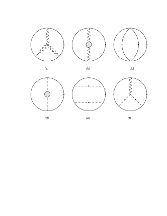
Figure 1: Non-vanishing two–loop diagrams for $\psi_{1}$ and $\psi_{2}$ loops. Wavy lines represent gauge propagators, solid lines represent scalars, and dashed lines are fermion propagators. Bubbles represent one–loop corrections to the propagators, as given in Appendix.

Diagram (a) - It comes from the gauge part of the third order expansion of the WL contracted with the gauge cubic vertex. Summing the contributions from the two connections $A_{(1)}$ and $A_{(2)}$, we have

$${\rm(a)}_{\psi_{1}}=-\frac{N_{1}(N_{1}^{2}-1)+N_{2}(N_{2}^{2}-1)}{N_{1}+N_{2}}\,\frac{1}{k^{2}}\,\frac{\Gamma^{3}(\frac{3}{2}-\epsilon)}{8\pi^{\frac{9}{2}-3\epsilon}}\,I^{(a)}$$ (23)

where

$$I^{(a)}=\int d\tau_{1>2>3}\,\dot{x}_{1}^{\sigma}\dot{x}_{2}^{\eta}\,\dot{x}_{3}^{\zeta}\,\varepsilon^{\xi\tau\kappa}\varepsilon_{\sigma\xi\mu}\varepsilon_{\eta\tau\nu}\varepsilon_{\zeta\kappa\rho}\times$$

$$\int d^{3-2\epsilon}x\frac{(x-x_{1})^{\mu}(x-x_{2})^{\nu}(x-x_{3})^{\rho}}{|x-x_{1}|^{3-2\epsilon}|x-x_{2}|^{3-2\epsilon}|x-x_{3}|^{3-2\epsilon}}$$ (24)

This integral, being finite, can be computed at $\epsilon=0$ and eventually gives $I^{(a)}=\frac{8}{3}\pi^{3}$ Rey:2008bh ; Bianchi:2013rma . The final result is then

$${\rm(a)}_{\psi_{1}}=-\frac{1}{24}\,\frac{N_{1}^{2}+N_{2}^{2}-N_{1}N_{2}-1}{k^{2}}$$ (25)

Diagrams (b) + (c) - Summing the two contributions we obtain

$$[{\rm(b)+(c)}]_{\psi_{1}}=$$

$$\frac{N_{1}^{2}(N_{0}+N_{2})+N_{2}^{2}(N_{1}+N_{3})}{N_{1}+N_{2}}\,\frac{1}{k^{2}}\,\frac{\Gamma^{2}(\frac{1}{2}-\epsilon)}{8\pi^{3-2\epsilon}}\,I^{(b+c)}$$

where Rey:2008bh

$$I^{(b+c)}=\int d\tau_{1>2}\,\frac{-\dot{x}_{1}\cdot\dot{x}_{2}+|\dot{x}_{1}||\dot{x}_{2}|}{[(x_{1}-x_{2})^{2}]^{1-2\epsilon}}\underset{\epsilon\rightarrow 0}{\longrightarrow}\pi^{2}$$ (27)

We then obtain

$$[{\rm(b)+(c)}]_{\psi_{1}}=\frac{N_{1}^{2}(N_{0}+N_{2})+N_{2}^{2}(N_{1}+N_{3})}{N_{1}+N_{2}}\,\frac{1}{8k^{2}}$$ (28)

Diagram (d) - This contribution is proportional to the exchange of a one–loop fermion propagator. Using its explicit expression given in Bianchi:2013rma we obtain

$${\rm(d)}_{\psi_{1}}\sim\int d\tau_{1>2}\,\frac{|\dot{x}_{1}||\dot{x}_{2}|}{[(x_{1}-x_{2})^{2}]^{1-2\epsilon}}\,\left[(c_{1}\bar{c}_{2})-(c_{2}\bar{c}_{1})\right]$$ (29)

where we indicate $c_{i}\equiv c(\tau_{i})$ on the circle. As follows from eq. (II) we have

$$(c_{i}\bar{c}_{j})=-\tfrac{2i}{k}\cos{\tfrac{\tau_{i}-\tau_{j}}{2}}$$ (30)

so that diagram (d) vanishes identically.

Diagram (e) - Expanding the $\psi_{1}$–loop at forth order and performing the two possible contractions of fermions we obtain a linear combination of terms of the form

$$\frac{\Gamma^{2}(\frac{3}{2}-\epsilon)}{4\pi^{3-2\epsilon}}\!\!\int\!\!d\tau_{1>..>4}\frac{(c_{i}\gamma^{\mu}\bar{c}_{j})(c_{k}\gamma^{\nu}\bar{c}_{l})(x_{i}-x_{j})_{\mu}(x_{k}-x_{l})_{\nu}}{[(x_{i}-x_{j})^{2}(x_{k}-x_{l})^{2}]^{\frac{3}{2}-\epsilon}}$$ (31)

This expression can be easily elaborated by using identity (21) twice. The contour integrals we are left with are divergent. They can be evaluated away from $\epsilon=0$ and suitably continued close to the origin (see Bianchi:2013rma for details). The result is

$${\rm(e)}_{\psi_{1}}=\frac{3}{8}\,\frac{N_{1}N_{2}}{k^{2}}$$ (32)

Diagram (f) - Expanding $W_{\psi_{1}}$ at third order and contracting with one mixed vertex $\bar{\psi}\psi A$ coming from the action, we obtain the linear combination of six integrals of the form

$$\frac{1}{k}\,\frac{\Gamma^{3}(\frac{1}{2}-\epsilon)}{64\pi^{\frac{9}{2}-3\epsilon}}\int d\tau_{1>2>3}(\bar{c}_{i}\gamma^{\xi}\gamma^{\mu}\gamma^{\sigma}c_{j})\,\dot{x}_{k}^{\nu}\,\varepsilon_{\nu\mu}^{\phantom{\nu\mu}\rho}\,\Gamma_{\rho\xi\sigma}$$ (33)

where the labels $i,j,k$ run over $1,2,3$ and

$$\Gamma^{\mu\nu\rho}\,=\,\partial^{\mu}_{k}\,\partial^{\nu}_{i}\,\partial^{\rho}_{j}\,\int\frac{d^{3}x}{[(x-x_{1})^{2}(x-x_{2})^{2}(x-x_{3})^{2}]^{\frac{1}{2}-\epsilon}}$$

The spinorial structure appearing in (33) can be simplified by using standard identities for the product of three Pauli matrices. It is easy to prove that, because of the planarity of the contour the only non–vanishing contributions we are left with are proportional to the bilinears $(c_{i}\bar{c}_{j})$ and $(c_{i}\gamma^{3}\bar{c}_{j})$. Using identity (30) together with

$$(c_{i}\gamma^{3}\bar{c}_{j})=\tfrac{2}{k}\sin{\tfrac{\tau_{1}-\tau_{2}}{2}}\quad,$$ (34)

computing the corresponding color factors and evaluating the integrals using the procedure described in Bianchi:2013rma we finally obtain

$${\rm(f)}_{\psi_{1}}=-\frac{1}{2}\,\frac{N_{1}N_{2}}{k^{2}}$$ (35)

Summing all the contributions the two–loop result for the $\psi_{1}$–loop is

$$\langle W_{\psi_{1}}[\Gamma]\rangle|_{\rm 2loop}=$$ (36)

$$1-\frac{1}{24k^{2}}\left[(N_{1}^{2}+N_{2}^{2}-N_{1}N_{2}-1)-3\frac{N_{0}N_{1}^{2}+N_{3}N_{2}^{2}}{N_{1}+N_{2}}\right]$$

We now consider the Wilson loop $W_{\psi_{2}}$ defined in (14, II). Its perturbative evaluation can be easily performed by exploiting the previous results, where we should take into account that the $\psi_{2}$–loop has slightly different scalar couplings in the ${\cal A}$–terms and different fermionic couplings $c,\bar{c}$. The fact that the $\psi_{(1)\hat{2}}$ fermion replaces $\psi_{(1)\hat{1}}$ does not make much difference, as the tree–level propagator for the two fermionic components is the same.

At one loop, the fermion exchange diagram (see equation (20)) involves the bilinear $(c_{i}\gamma^{\mu}\bar{c}_{j})(x_{i}-x_{j})_{\mu}$. Computing it with the assignment (II), we obtain the same result (21) up to an overall sign. However, since the diagram is still proportional to integral (22), the $\psi_{2}$–loop contribution at one loop also vanishes in the $\epsilon\to 0$ limit.

At two loops, non–vanishing contributions are still given in Fig. 1. It is easy to argue that the first three bosonic diagrams give the same result as $W_{\psi_{1}}$. In fact, diagram (a) and (b) involve only gauge fields, so they are insensitive to changes in matter couplings. In diagram (c) the matrices ($I$ and $\sigma_{3}$) governing the scalar couplings enter quadratically, so that the sign difference between the two WL definitions does not affect the calculation. Changes in the calculation might be expected from diagrams containing fermions, since a different set of fermionic couplings may give rise to different expressions for the fermionic bilinears $(c_{i}\bar{c}_{j})$ and $(c_{i}\gamma^{\mu}\bar{c}_{j})$. However, the contribution from diagram (d) is still proportional to expression (29) and vanishes since, as before, $(c_{1}\bar{c}_{2})=(c_{2}\bar{c}_{1})$, as follows immediately from (II). In diagram (e) the double fermion contractions read again as in eq. (31), which involves the bilinear $(c_{i}\gamma^{\mu}\bar{c}_{j})(x_{i}-x_{j})_{\mu}$. As we already mentioned, this bilinear has an overall sign compared to the corresponding expression for $W_{\psi_{1}}$. However, in (31) the product of two such expressions appears, so that the final result is the same as for $W_{\psi_{1}}$. Finally, diagram (f) only involves minimal coupling of fermions to the gauge vectors, which is identical for $\psi_{(1)\hat{1}}$ and $\psi_{(1)\hat{2}}$. Therefore the evaluation of the integrals still depends on the spinorial bilinears $(c_{i}\bar{c}_{j})$ and $(c_{i}\gamma^{3}\bar{c}_{j})$. Using (II), these can be quickly shown to be identical to the ones for the $\psi_{1}$–loop. Here it is crucial that, due to the planarity of the contour, only the bilinear $(c_{i}\gamma^{\mu}\bar{c}_{j})$ with $\mu=3$ enters the calculation. If this were not the case, we would obtain a different result, since for the bilinears along the directions $\mu=1,2$ where the circular contour lies there is a sign difference between the two WL.

Summarizing, we find that

$$\langle W_{\psi_{1}}[\Gamma]\rangle|_{\rm 2loop}=\langle W_{\psi_{2}}[\Gamma]\rangle|_{\rm 2loop}$$ (37)

Therefore, up to this order, there is no quantum uplift of the degeneracy between the two fermionic WL.

Exploiting the previous calculation, it is also immediate to determine the $1/4$ bosonic WLs (II). Again, there is no one–loop contribution, while the two–loop ones are given by the first three diagrams in Fig. 1. With suitable adjustments we find ($A=1,2$)

$$\langle W^{(A)}\rangle=1-\frac{1}{24k^{2}}\left[N_{A}^{2}-3N_{A-1}N_{A}-3N_{A}N_{A+1}-1\right]$$

Note that, under identification $N_{0}=N_{2}$ and $N_{3}=N_{1}$, our results (36, III) coincide with the two–loop expressions for the $1/2$ and $1/6$ Wilson loops in ABJ, respectively Drukker:2009hy ; Rey:2008bh ; Bianchi:2013rma ; Griguolo:2013sma . Moreover, in the orbifold ABJM $[U(N)\times U(N)]^{r}$ ($N_{A}=N$ for all the nodes) the result becomes

$$\langle W_{\psi_{1}}\rangle\Big{|}_{\rm 2loop} =\langle W_{\psi_{2}}\rangle\Big{|}_{\rm 2loop}$$

$$=1+\frac{1}{24k^{2}}\left(2N^{2}+1\right)\sim\frac{1}{12}\left(\frac{N}{k}\right)^{2}$$

$$\langle W^{(1,2)}\rangle|_{\rm 2loop}=1+\frac{1}{24k^{2}}\left(5N^{2}+1\right)\sim\frac{5}{24}\left(\frac{N}{k}\right)^{2}$$

IV Cohomological equivalence at quantum level

It is easy to generalize the results (36) to a generic $A$ site ($A=0,\cdots,2r-1$) and write

$$\langle W_{\psi_{i}}^{(A)}\rangle|_{i=1,2}=1-\frac{1}{24k^{2}}\Big{[}N_{A}^{2}+N_{A+1}^{2}-N_{A}N_{A+1}-1$$

$$\qquad\qquad\qquad\,\,-3\frac{N_{A-1}N_{A}^{2}+N_{A+2}N_{A+1}^{2}}{N_{A}+N_{A+1}}\Big{]}+\cdots$$ (40)

Similarly, generalizing result (III), for bosonic WL related to the $A$ site we have

$$\langle W^{(A)}\rangle=1-$$ (41)

$$\qquad\frac{1}{24k^{2}}\left[N_{A}^{2}-3N_{A-1}N_{A}-3N_{A}N_{A+1}-1\right]+\cdots$$

Exploiting these results it is interesting to understand how the classical cohomological equivalence (19) gets enhanced at quantum level. In fact, comparing the previous expressions one can easily realize that the following identity holds

$$\langle W_{\psi_{i}}^{(A)}\rangle_{0}=e^{-i\frac{\ell_{A}}{2k}(N_{A}-N_{A+1})}\times$$ (42)

$$\frac{N_{A}\,e^{i\frac{\ell_{A}}{2k}N_{A}}\langle W^{(A)}\rangle_{0}+N_{A+1}\,e^{-i\frac{\ell_{A}}{2k}N_{A+1}}\langle W^{(A+1)}\rangle_{0}}{N_{A}+N_{A+1}}$$

where $\ell_{A}=(-1)^{A+1}$ and the subscript “0” means perturbative result (framing zero). Therefore, if we define “framing–one” quantities

$$\langle W_{\psi_{i}}^{(A)}\rangle_{1}=e^{i\frac{\ell_{A}}{2k}(N_{A}-N_{A+1})}\,\langle W_{\psi_{i}}^{(A)}\rangle_{0}\qquad j=1,2$$

$$\langle W^{(A)}\rangle_{1}=e^{-i\frac{\ell_{A}}{2k}N_{A}}\langle W^{(A)}\rangle_{0}$$ (43)

the previous identity can be rewritten as

$$\langle W_{\psi_{i}}^{(A)}\rangle_{1}=\frac{N_{A}\langle W^{(A)}\rangle_{1}+N_{A+1}\langle W^{(A+1)}\rangle_{1}}{N_{A}+N_{A+1}}$$ (44)

and looks exactly like the classical relation (19).

V Matrix Model result at weak coupling

We now discuss the matrix model for the necklace quiver theory described in Section II. The putative matrix integral, which yields the partition function, can be easily obtained by combining the basic building blocks given in Kapustin:2009kz . We find Marino:2012az

$$\mathcal{Z}\!=\!\mathcal{N}\!\!\int\!\!\prod_{B,i}{d\lambda_{Bi}}e^{2ik\ell_{B}\lambda_{Bi}^{2}}\!\prod_{B=0}^{2r-1}\frac{\prod_{i<j}\sinh^{2}\left(\lambda_{Bi}-\lambda_{Bj}\right)}{\prod_{i,j}\cosh\left(\lambda_{Bi}-\lambda_{B+1,j}\right)}$$ (45)

The constant $\mathcal{N}$ is an overall normalization, whose explicit form is irrelevant in our computation.

In the matrix model language the $1/2$ BPS Wilson loop is not a fundamental object, as it can be computed from the $1/4$ BPS Wilson loop through the cohomological relation (44). Therefore we focus on the latter. It is given by the vacuum expectation value of the following matrix observable

$$\!\!W^{(A)}\!= \frac{1}{N_{A}}\sum_{i=1}^{N_{A}}e^{2\lambda_{Ai}}=1\!+\!\frac{2}{N_{A}}\text{Tr}(\Lambda_{A})\!+\!\frac{2}{N_{A}}\text{Tr}(\Lambda^{2}_{A})+\!$$

$$+\frac{4}{3N_{A}}\text{Tr}(\Lambda_{A}^{3})+\frac{2}{3N_{A}}\text{Tr}(\Lambda^{4}_{A})+O\left(\Lambda_{A}^{5}\right)$$ (46)

where we have introduced the diagonal matrix $\Lambda_{A}\equiv\text{diag}(\lambda_{A1},\cdots,\lambda_{AN_{A}})$ for future convenience. In the r.h.s. of (V) we can actually neglect all the odd powers in $\Lambda_{A}$ since their expectation value vanishes at all order in $\frac{1}{k}$ due to the symmetry property of the integrand in (45) under the parity transformation $\lambda_{Ai}\to-\lambda_{Ai}$.

In order to construct the perturbative series for $W^{(A)}$, first we rescale the eigenvalues $\lambda_{Ai}$ with $\frac{1}{\sqrt{k}}$. Therefore, the measure factor for large $k$ reads

$$\prod_{B=0}^{2r-1}\frac{\prod_{i<j}\sinh^{2}\frac{\lambda_{Bi}-\lambda_{Bj}}{\sqrt{k}}}{\prod_{i,j}\cosh\frac{\lambda_{Bi}-\lambda_{B+1,j}}{\sqrt{k}}}=$$ (47)

$$\left[1+\frac{1}{k}\sum_{B=0}^{2r-1}P_{B}+O\left(\frac{1}{k^{2}}\right)\right]\prod_{B=0}^{2r-1}\prod_{i<j}\frac{(\lambda_{Bi}-\lambda_{Bj})^{2}}{k}$$

where

$$P_{B}\equiv \frac{1}{3}(N_{B}\mathrm{Tr}(\Lambda_{B}^{2})-\mathrm{Tr}(\Lambda_{B})^{2})-\frac{1}{2}(N_{B+1}\!\mathrm{Tr}(\Lambda_{B}^{2})\!+$$

$$+\!N_{B}\!\mathrm{Tr}(\Lambda_{B+1}^{2})\!-\!2\mathrm{Tr}(\Lambda_{B})\mathrm{Tr}(\Lambda_{B+1})).$$ (48)

Since we shall write the final result as a combination of vacuum expectation values in the Gaussian matrix model, we have chosen to use the usual Vandermonde determinant as the reference measure. Moreover we have not explicitly written $\tfrac{1}{k^{2}}$ terms since they do not affect the final result. In fact, they cancel out with the normalization provided by the partition function.

With the help of the expansion (47), it is straightforward to write down the expectation value of the Wilson loop $W^{(A)}$ in terms of $P_{B}$ and $\Lambda_{A}$. We find

$$\begin{split}&\langle W^{(A)}\rangle=1\!+\!\frac{2}{N_{A}k}\langle\mathrm{Tr}(\Lambda^{2}_{A})\rangle\!+\!\frac{1}{N_{A}k^{2}}\left[\frac{2}{3}\langle\mathrm{Tr}(\Lambda^{4}_{A})\rangle+\right.\\ &\left.+2\sum_{B=0}^{2r-1}\left[\langle\mathrm{Tr}(\Lambda^{2}_{A})P_{B}\rangle-\langle\mathrm{Tr}(\Lambda^{2}_{A})\rangle\langle P_{B}\rangle\right]\right]\!+\!O\left(\frac{1}{k^{3}}\right),\\ \end{split}$$ (49)

where all the expectation values in the r.h.s. of eq. (49) are taken in Gaussian matrix model of coupling constant $(-2i\ell_{B})$. At the order $\frac{1}{k^{2}}$ the effect of the interactions is entirely encoded in the combination $\langle\mathrm{Tr}(\Lambda^{2}_{A})P_{B}\rangle-\langle\mathrm{Tr}(\Lambda^{2}_{A})\rangle\langle P_{B}\rangle$. However this combination vanishes unless $B=A-1$ or $B=A$ and thus the Wilson loop receives contributions from the nodes $A-1$, $A$ and $A+1$ (we recall that $P_{B}$ also depends on $\Lambda_{B+1}$). This is similar to what occurs in ABJ theories with the difference that the node $A-1$ and $A+1$ are identified there.

Using known results on the expectation values of $\mathrm{Tr}(\Lambda^{n})$ and on correlators of traces in the Gaussian matrix model, we finally find

$$\langle W^{(A)}\rangle=1+\frac{i\ell_{A}N_{A}}{2k}-$$ (50)

$$-\frac{1}{24k^{2}}(4N_{A}^{2}-3N_{A-1}N_{A}-3N_{A+1}N_{A}-1)+O\left(\frac{1}{k^{3}}\right)$$

This expression coincides with the perturbative result for ${1/4}$ BPS Wilson loop given in (III) dressed with the phase (IV) corresponding to framing $1$. With the help of cohomological relation (44), we can also build $\langle W^{(A)}_{\psi_{i}}\rangle$ and we find again the same result (IV) of the perturbative computation.

VI Discussion and perspectives

We have studied the two-loop perturbative behavior of the 1/2 BPS Wilson loop operators $W_{\psi_{1}}$ and $W_{\psi_{2}}$ introduced in Ouyang:2015qma ; Cooke:2015ila in the case of $\mathcal{N}=4$ Chern-Simons matter quiver theories with alternating levels.

The Feynman diagram analysis of Section III has shown that up to two loops the expectation values of $W_{\psi_{1}}$ and $W_{\psi_{2}}$ are coincident and match the prediction from the perturbative expansion of the matrix model obtained in Section IV. Remarkably, in the field theory computation the coincidence between the two Wilson loops is true not only for the full result but it holds also for each of the contributing diagrams. At this perturbative order the two Wilson loops share exactly the same properties. We thus have to go up to three loops to look for hints of a possible lifting of the degeneracy between the two classically equivalent 1/2 BPS operators.

Indeed, at three loops some distinctive features in the perturbative computation arise. First of all, at this order the two Wilson loops start giving different results at the level of single diagrams. It is easy to find examples of this behaviour and we provide the simplest one in Fig 2.

Evaluating the diagram for the two Wilson loops we obtain

$$W_{\psi_{2}}|_{\rm Fig.2}=-W_{\psi_{1}}|_{\rm Fig.2}$$ (51)

with

$$W_{\psi_{1}}|_{\rm Fig.2}=-\frac{2}{k^{3}}\frac{N_{1}N_{2}(N_{1}^{2}+N_{2}^{2}+2)}{N_{1}+N_{2}}\,\,\textrm{I}(\epsilon)$$ (52)

$$\textrm{I}(\epsilon)=\frac{4}{3}\,\Gamma\left(-\tfrac{1}{2}+3\epsilon\right)\left[\frac{\Gamma(\tfrac{1}{2}-\epsilon)\Gamma(1+\epsilon)}{(4\pi)^{1-\epsilon}\Gamma(1+2\epsilon)}\right]^{3}\underset{\epsilon\rightarrow 0}{\longrightarrow}-\frac{1}{24\pi}$$

The extra minus sign in $W_{\psi_{2}}$ compared to $W_{\psi_{1}}$ comes from the different scalar couplings in the two Wilson loop definitions. This situation is very similar to what happens for the one-loop fermion exchange contribution of Section III. However, while in that case the diagram is eventually discarded because the integral has been shown to be $\mathcal{O}(\epsilon)$, in the present case a finite contribution survives in the $\epsilon\to 0$ limit.

Figure 2: Example of a three-loop diagram yelding different results for $W_{\psi_{1}}$ and $W_{\psi_{2}}$.

Another source of possible differences might come from the Yukawa vertices in the potential, which start contributing at three loops. In fact, while minimal couplings entering up to two loops are diagonal in the flavour space, Yukawa vertices are in general flavour changing and the computation might become sensible to the flavour choice of the spinor insertions on the contour.

Based on these general observations, we expect a different result for a subset of three–loop Feynman diagrams and it would be crucial to check if the differences are compensated when we sum over all the contributions. If this were the case, the common result of the two operators should match the three-loop expansion of the matrix model. Instead, if the differences would not cancel against each others, and cannot be absorbed in a change of framing, the prediction from the matrix model could be matched only by a specific linear combination of the two Wilson loops, as suggested in Cooke:2015ila . A more radical possibility is that no linear combination satisfies the constraint and therefore the cohomological equivalence is broken at the quantum level. We will report on the ongoing three–loop analysis in forthcoming .

Moreover, it would be interesting to understand how the $W_{\psi_{i}}$ operators of the $\mathcal{N}=4$ models fit in the family of 1/2 BPS Wilson loops recently introduced Ouyang:2015iza for general $\mathcal{N}=2$ theories, where a perturbative analysis such as the one completed in this paper could also be applied.

VII Acknowledgements

This work has been supported in part by MIUR, INFN and MPNS-COST Action MP1210 “The String Theory Universe”.

References

- (1) J. K. Erickson, G. W. Semenoff and K. Zarembo, Nucl. Phys. B 582 (2000) 155 [hep-th/0003055].
- (2) N. Drukker and D. J. Gross, J. Math. Phys. 42, 2896 (2001) [hep-th/0010274].
- (3) V. Pestun, Commun. Math. Phys. 313 (2012) 71 [arXiv:0712.2824 [hep-th]].
- (4) N. Drukker, S. Giombi, R. Ricci and D. Trancanelli, JHEP 0805 (2008) 017 [arXiv:0711.3226 [hep-th]].
- (5) A. Kapustin, B. Willett and I. Yaakov, JHEP 1003 (2010) 089 [arXiv:0909.4559 [hep-th]].
- (6) N. Drukker and D. Trancanelli, JHEP 1002 (2010) 058 [arXiv:0912.3006 [hep-th]].
- (7) V. Cardinali, L. Griguolo, G. Martelloni and D. Seminara, Phys. Lett. B 718, 615 (2012) arXiv:1209.4032 [hep-th].
- (8) N. Drukker, M. Marino and P. Putrov, Commun. Math. Phys. 306 (2011) 511 [arXiv:1007.3837 [hep-th]].
- (9) H. Ouyang, J. B. Wu and J. j. Zhang, arXiv:1506.06192 [hep-th].
- (10) M. Cooke, N. Drukker and D. Trancanelli, JHEP 1510 (2015) 140 [arXiv:1506.07614 [hep-th]].
- (11) D. Gaiotto and E. Witten, JHEP 1006 (2010) 097 [arXiv:0804.2907 [hep-th]].
- (12) K. Hosomichi, K. M. Lee, S. Lee, S. Lee and J. Park, JHEP 0807 (2008) 091 [arXiv:0805.3662 [hep-th]].
- (13) M. S. Bianchi, G. Giribet, M. Leoni and S. Penati, JHEP 1310 (2013) 085 [arXiv:1307.0786 [hep-th]].
- (14) L. Griguolo, G. Martelloni, M. Poggi and D. Seminara, JHEP 1309 (2013) 157 [arXiv:1307.0787 [hep-th]].
- (15) S. -J. Rey, T. Suyama and S. Yamaguchi, JHEP 0903 (2009) 127 [arXiv:0809.3786 [hep-th]].
- (16) M. Mariño and P. Putrov, JHEP 1311, 199 (2013) [arXiv:1206.6346 [hep-th]].
- (17) H. Ouyang, J. B. Wu and J. j. Zhang, arXiv:1507.00442 [hep-th].
- (18) Y. Imamura and K. Kimura, JHEP 0810 (2008) 040 [arXiv:0807.2144 [hep-th]].
- (19) M.S. Bianchi, L. Griguolo, M. Leoni, A. Mauri, S. Penati and D. Seminara, in preparation.
- (20) H. Ouyang, J. B. Wu and J. j. Zhang, arXiv:1510.05475 [hep-th].