Second Order Calibration: A Simple Way to Get Approximate Posteriors

Abstract.

Many large-scale machine learning problems involve estimating an unknown parameter $\theta_{i}$ for each of many items. For example, a key problem in sponsored search is to estimate the click through rate (CTR) of each of billions of query-ad pairs. Most common methods, though, only give a point estimate of each $\theta_{i}$. A posterior distribution for each $\theta_{i}$ is usually more useful but harder to get.

We present a simple post-processing technique that takes point estimates or scores $t_{i}$ (from any method) and estimates an approximate posterior for each $\theta_{i}$. We build on the idea of calibration, a common post-processing technique that estimates $\mathrm{E}\left(\theta_{i}\!\!\bigm{|}\!\!t_{i}\right)$. Our method, second order calibration, uses empirical Bayes methods to estimate the distribution of $\theta_{i}\!\!\bigm{|}\!\!t_{i}$ and uses the estimated distribution as an approximation to the posterior distribution of $\theta_{i}$. We show that this can yield improved point estimates and useful accuracy estimates. The method scales to large problems - our motivating example is a CTR estimation problem involving tens of billions of query-ad pairs.

1. Introduction

Suppose we have a regression problem: we have responses $y_{i}$ and covariates $\boldsymbol{x}_{i}$ for items $i=1,\ldots,I$, and we want to estimate a parameter $\theta_{i}$ for each item using our responses and covariates. We often want a posterior distribution for each $\theta_{i}$, but common regression methods, like neural networks, boosted trees and penalized GLMs, only give us point estimates $t_{i}=t\left(\boldsymbol{x}_{i}\right)$. In this paper, we show how to post-process any regression method’s point estimates to get an approximate posterior.

Our motivating problem is click through rate (CTR) estimation for sponsored search (Richardson et al., 2007). Here, our items are query-ad pairs, and for each pair, we know the number of times it was shown (the number of “impressions”, $N_{i}$), the number of times it was clicked ($y_{i}$), and covariates that describe the query, ad and match between them, ($\boldsymbol{x}_{i}$). We assume the clicks for each query-ad pair follow a Poisson distribution:

$$y_{i}\sim\mathrm{Poisson}\left(\theta_{i}N_{i}\right)$$

and want to estimate $\theta_{i}$, the CTR for the query-ad pair. A complex machine learning system gives us point estimates $t_{i}$. We want a posterior distribution for each $\theta_{i}$. Among other things, we could use these posteriors to make fine-grained accuracy estimates and explore-exploit tradeoffs.

Any method to get posteriors for the CTR problem has to have three important features. First, it has to scale. Search engines have billions of query-ad pairs. Second, it cannot depend on the underlying machine learning system that gives $t_{i}$. CTR estimation systems are complex - not least because of their scale - and are constantly being improved (Graepel et al., 2010). If a method used detailed knowledge of the system to get posteriors, it would have to account for all the complexity and be updated constantly as the system changed; we also wouldn’t be able to use its posteriors to compare the system to a very different competitor. Third, the method must share information across query-ad pairs. Because of the long-tail nature of search queries, most query-ad pairs are shown a small number of times. This, combined with CTRs that are generally low, means that taken individually, most query-ad pairs have little information.

We get approximate posteriors by extending the idea of calibration, a common post-processing technique that removes bias from regression estimates. There are a few different methods for calibration, but all are based the same idea: instead of using $t$, estimate and use $\mathrm{E}\left(\theta\!\!\bigm{|}\!\!t\right)$ (we’ll drop the subscripts from now on, when the meaning is clear). In the CTR estimation problem, for example, we can estimate $\mathrm{E}\left(\theta\!\!\bigm{|}\!\!t=t_{0}\right)$ using the average CTR of query-ad pairs with $t$ close to $t_{0}$. Calibration can improve any regression method’s estimates by removing any aggregate bias. This lets us use methods that, because of regularization, other bias-variance tradeoffs, or model mis-specification, are efficient but biased. We can also use calibration to turn scores, that are not estimates of $\theta$ but have information about $\theta$, into estimates of $\theta$ without aggregate bias. Finally, calibration satisfies the three requirements for the CTR estimation problem - it scales easily, it doesn’t depend on the underlying system, and it shares information by using all the items with a similar $t$ to estimate the correction at that $t$.

Calibration estimates $\mathrm{E}\left(\theta\!\!\bigm{|}\!\!t\right)$. We propose estimating the distribution of $\theta\!\!\bigm{|}\!\!t$, and using this to approximate the distribution of $\theta\!\!\bigm{|}\!\!\boldsymbol{x}$. Figure 1 illustrates the idea by plotting $\theta$ vs $t$. Calibration adjusts our estimate, as a function of $t$, by moving from the $x=y$ line to the conditional mean curve $\mathrm{E}\left(\theta\!\!\bigm{|}\!\!t\right)$. The proposed method, which we call second order calibration, goes further and estimates the distribution of $\theta$ around that curve. We don’t observe the true $\theta$, so we can’t estimate the distribution of $\theta\!\!\bigm{|}\!\!t$ directly. But if many items have an estimate close to $t$, we can estimate the $\theta\!\!\bigm{|}\!\!t$ distribution by using the observed $y$s for those nearby items and employing standard empirical Bayes techniques. Like ordinary calibration, our method can also be used when $t$ is a score that has information about $\theta$, rather than itself an estimate of $\theta$, though for this paper, we assume $t$ is an estimate of $\theta$.

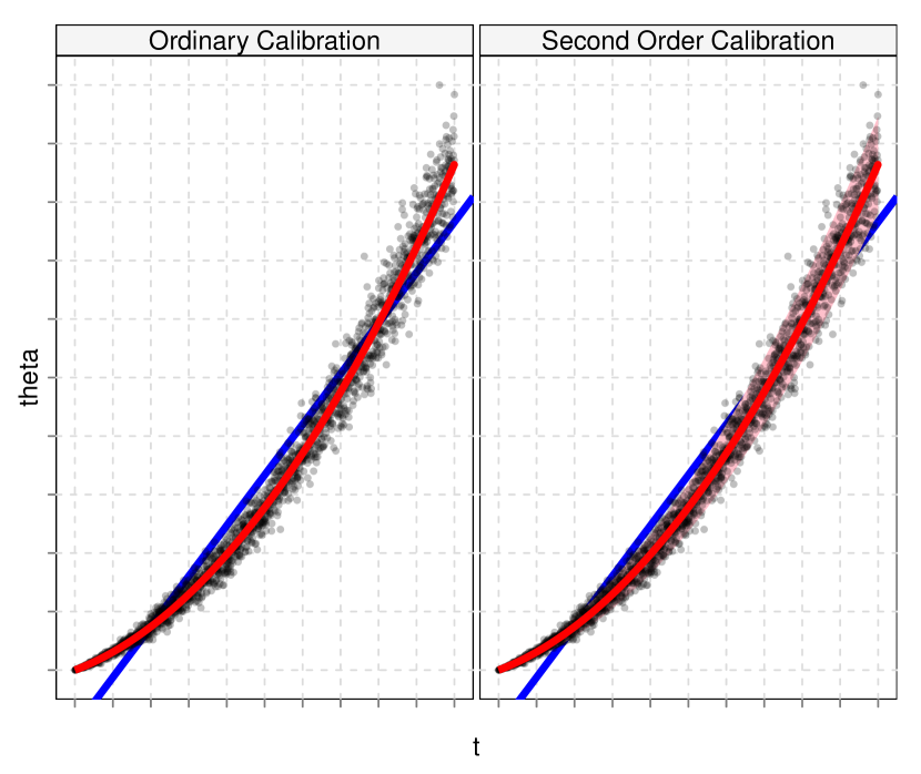
Figure 1. Ordinary and second order calibration. Each panel plots $\theta$ on the $y$-axis against $t$ on the $x$-axis. Ordinary calibration, left, adjusts our estimate from $t$ (the blue line, $x=y$) to $\mathrm{E}\left(\theta\!\!\bigm{|}\!\!t\right)$ (the red line). Second order calibration, right, goes further. It uses $y$ to estimate the distribution of $\theta\!\!\bigm{|}\!\!t$ (represented by the pink color strip), and uses that distribution to estimate $\mathrm{Var}\left(\theta\!\!\bigm{|}\!\!t\right)$, $\mathrm{E}\left(\theta\!\!\bigm{|}\!\!t,y\right)$ and $\mathrm{Var}\left(\theta\!\!\bigm{|}\!\!t,y\right)$.

How is this useful? Although we think approximate posteriors will be useful in many ways, we focus on three applications: overall accuracy estimation, improved point estimates, and fine-grained accuracy estimation.

Overall Accuracy Estimation

Second order calibration estimates $\mathrm{Var}\left(\theta\!\!\bigm{|}\!\!t\right)$, which measures the accuracy of the estimation system (if $t$ is a score, this measures the accuracy of the calibrated score). This lets us separate errors due to noise, which would happen even with perfect parameter estimates, from errors in estimation. Separating these errors can be valuable. For example, consider the CTR estimation problem. Because of the Poisson noise, we cannot make perfect predictions even if we estimate $\theta$ perfectly for each query-ad pair. If we have an estimation system that predicts badly, second order calibration can tell us whether this is because the system is inaccurate and can be improved, or whether it is predicting as well as the noise will allow.

Improved Point Estimates

Second order calibration can improve point estimates through better shrinkage. Suppose that for each item $i$, $t_{i}$ is trained on data independent of $y_{i}$; we can do this by dividing our data into multiple folds, like in cross-validation, and would need to do this anyway for ordinary calibration. Ordinary calibration improves on $t$ by using $\mathrm{E}\left(\theta\!\!\bigm{|}\!\!t\right)$ instead. We can do even better by using $\mathrm{E}\left(\theta\!\!\bigm{|}\!\!t,y\right)$. This estimator essentially decomposes memorization and generalization. The underlying regression method handles generalization: the distribution of $\theta\!\!\bigm{|}\!\!t$ reflects what we know about $\theta$ based on $t$, the underlying regression method’s summary of the information in $\boldsymbol{x}$ and the other items. Second order calibration then handles memorization by combining $\theta\!\!\bigm{|}\!\!t$ with the item-specific information in $y$. By estimating the distribution of $\theta\!\!\bigm{|}\!\!t$, we can often combine the two sources of information close to optimally. Requiring $t_{i}$ not be trained on $y_{i}$ makes sure we don’t double count the information in $y_{i}$. In practice, this condition can be relaxed: $t_{i}$ can be trained on $y_{i}$ as long as $y_{i}$ does not influence $t_{i}$ too much.

Decomposing memorization and generalization can be much better than letting the underlying estimation system train on all the data and handle both memorization and generalization. More interestingly, we could design our estimation system to work with this decomposition. For example, we could use a relatively coarse generalization model to generate $t$ and memorize item-specific information using $\mathrm{E}\left(\theta\!\!\bigm{|}\!\!t,y\right)$.

Fine-Grained Accuracy Estimation

Second order calibration can estimate our accuracy for each item. Again, suppose $t_{i}$ is trained on data independent of $y_{i}$ for each $i$ (or, in practice, that $y_{i}$ does not influence $t_{i}$ too much). We can use $\mathrm{Var}\left(\theta\!\!\bigm{|}\!\!t,y\right)$ to measure the accuracy of $\mathrm{E}\left(\theta\!\!\bigm{|}\!\!t,y\right)$, and as a general measure of how much we know about each item. Second order calibration gives us estimates of $\mathrm{Var}\left(\theta\!\!\bigm{|}\!\!t,y\right)$, which we can use to make risk-adjusted decisions and explore-exploit tradeoffs, or to find where the underlying regression method is particularly good or bad.

Worries and Limitations

We might worry that there just isn’t enough information in the $y$s to get a useful estimate of the distribution of $\theta\!\!\bigm{|}\!\!t$. If this were true, second order calibration could never be useful. Fortunately, this is not the case for each of the three applications above. We prove as long as our estimate of the distribution of $y\!\!\bigm{|}\!\!t$ fits well, second order calibration will correctly estimate the true $\mathrm{Var}\left(\theta\!\!\bigm{|}\!\!t\right)$, $\mathrm{E}\left(\theta\!\!\bigm{|}\!\!t\right)$ and $\mathrm{Var}\left(\theta\!\!\bigm{|}\!\!t,y\right)$. We discuss a simple diagnostic to check the fit.

Like ordinary calibration, second order calibration is intended to be easy and useful, not comprehensive or optimal, and it shares some of ordinary calibration’s limitations. Both ordinary calibration and second order calibration require that each $t_{i}$ be trained on data independent of $y_{i}$. This is easy to achieve in principle with folds, but can be inconvenient; in practice, both methods work well if $y_{i}$ does not influence $t_{i}$ too much. Both methods can also be wrong for slices of the data while being correct on average, since they only use $\boldsymbol{x}$ through $t$. This is especially important for second order calibration, since we always approximate $\theta\!\!\bigm{|}\!\!\boldsymbol{x}$ using $\theta\!\!\bigm{|}\!\!t$. We can guard against this by calibrating separately for important classes of items (for example, we can calibrate CTR estimates separately for each country), but that cannot solve the problem completely.

Second order calibration also has another important limitation, not shared with ordinary calibration: we must have a known parametric model for the distribution of $y\!\!\bigm{|}\!\!\theta$. In our CTR example, for instance, $y\!\!\bigm{|}\!\!\theta$ is assumed to be $\mathrm{Poisson}\left(\theta N\right)$, with $N$ known. We need to know the noise mechanism to work backward from the observed distribution of the $y$s to the $\theta\!\!\bigm{|}\!\!t$ distribution. It can be hard to check whether our noise model is accurate - in our CTR example, we use predictive distributions to check the Poisson model indirectly. Also, although we expect second order calibration to work well for fairly general known noise, our theory only applies when the noise is Poisson or a continuous natural exponential family (e.g. normal with known variance).

The rest of this paper is organized as follows. We discuss related work in Section 2. We then present our method for second order calibration in Section 3, using CTR estimation to illustrate. In Section 4, we state a theoretical result justifying the three applications of second order calibration mentioned above. Finally, in Section 5, we present our results on the CTR estimation problem and on simulations. Proofs are in Appendix A.

2. Related work

Second order calibration is closely related to existing calibration and empirical Bayes methods.

2.1. Calibration

Calibration is usually used to post-process the output of good classifiers that produce bad class probability estimates (Niculescu-Mizil and Caruana, 2005). Cohen and Goldszmidt (2004) show that, in general, calibration does not reduce classification accuracy, and makes it easier to find the right threshold to minimize classification error. Calibration can be very effective: Caruana and Niculescu-Mizil (2006) show that it turns boosted trees into excellent probability estimators. The two most common methods for calibration are Platt scaling (Platt, 1999), which is equivalent to logistic regression, and isotonic regression (Zadrozny and Elkan, 2002).

Most of the literature on calibration discusses classifiers, but regression methods are commonly calibrated as well. Both isotonic regression and Platt scaling generalize straightforwardly to calibrating regression methods. Amini and Johnson (2009) use random effect methods to calibrate and estimate the accuracy of regression methods.

2.2. Empirical Bayes

Empirical Bayes methods use Bayesian inference to solve problems, but estimate priors instead of using subjective or reference priors. The key idea is that if we have many independent draws from a model with unknown prior, we can use the data to estimate the prior, or a quantity of interest that depends on the prior.

For example, suppose that $\mu$ comes from an unknown prior $G$, our data $z$ is $\mathcal{N}\left(\mu,1\right)$, and we observe many $z$s from this model. We want to say something about the unobserved $\mu_{i}$ corresponding to each $z_{i}$. As Robbins (1954) showed, we can use the $z$s to estimate the prior, then estimate $\mu_{i}$ using $\mathrm{E}_{\hat{G}}\left(\mu_{i}\!\!\bigm{|}\!\!z_{i}\right)$, where $\mathrm{E}_{\hat{G}}$ is the expectation in our model under the estimated prior $\hat{G}$. This estimate of $\mu_{i}$ combines global information from all the $z$s (via $\hat{G}$) with the specific information in $z_{i}$.

Emprical Bayes methods work when the quantity we’re interested in can be expressed in terms of the marginal density of the data. Such an expression tells us we can estimate the quantity, since we can estimate the marginal density using our data. In our normal example, Tweedie’s formula (Robbins, 1954) shows that if $f_{G}$ is the marginal density of the $z$s,

$$\mathrm{E}_{G}\left(\mu\!\!\bigm{|}\!\!z\right)=z-\frac{f_{G}^{\prime}\left(z\right)}{f_{G}\left(z\right)}$$

for any prior $G$ (Robbins actually estimated this quantity directly instead of using an estimate of the prior). Since we observe many $z$s, we can estimate the marginal and thus estimate $\mathrm{E}_{G}\left(\mu\!\!\bigm{|}\!\!z\right)$ without knowing the prior in advance.

Empirical Bayes methods need a large amount of data to shine. Big data sets have made them increasingly useful; Efron (2010) gives an introduction and review. They have enjoyed particular success recently in signal processing (e.g. (Johnstone and Silverman, 2004)) and multiple testing (though false discovery rates, e.g. (Efron et al., 2001)).

2.3. Why not bootstrap?

At first glance, the bootstrap seems like a natural way to get approximate posteriors for any regression method. Before we present second order calibration, it is worth understanding why the bootstrap doesn’t work for this problem. The bootstrap is often too slow for large data sets, since it requires training the regression method many times. In the CTR estimation problem, for example, bootstrapping would require training a massive, resource-intensive machine learning system tens or even hundreds of times. This is impractical and expensive. Post-processing methods like ordinary and second order calibration are much easier to use.

More importantly, though, the bootstrap estimates the distribution of $t$, not of $\theta\!\!\bigm{|}\!\!t$, and these distributions can be very different, particularly for the biased estimators often used on large data sets. Consider the trivial estimator $t=0$. The bootstrap would correctly find that $t$ is always $0$, but this tells us nothing about the distribution of $\theta\!\!\bigm{|}\!\!t$.

3. The Proposed Method

We now state the second order calibration problem more precisely. We are given responses $y_{i}$ for items $i=1,\ldots,I$. Each item has a parameter $\theta_{i}$ that controls the response in a known way: $y_{i}\!\!\bigm{|}\!\!\theta_{i}\sim f_{\theta_{i}}$, where $f_{\theta}$ is a given parametric family. The family $f_{\theta}$ can depend on known offsets that are different for each $i$; we suppress this dependence in our notation. We assume that $f_{\theta}$ is either Poisson ($y\!\!\bigm{|}\!\!\theta\sim\mathrm{Poisson}\left(N\theta\right)$) or a continuous exponential family with natural parameter $\theta$ (for example, $y\!\!\bigm{|}\!\!\theta\sim\mathcal{N}\left(\theta,\sigma^{2}\right)$ with known $\sigma$). For each item $i$, a machine learning system gives us an estimate $t_{i}$ that is not trained on $y_{i}$. Our goal is to estimate the posterior distribution $\theta\!\!\bigm{|}\!\!t$, which we denote by $G_{t}$, for each $t$.

We will use $G_{t}$ to approximate the full posterior distribution $\theta\!\!\bigm{|}\!\!\boldsymbol{x}$. The quality of this approximation will depend on the underlying machine learning method and the data set. In this paper, we will not try to quantify the approximation error. Our goal is to estimate functionals of the true $G_{t}$, which average the true $\theta\!\!\bigm{|}\!\!\boldsymbol{x}$ distributions, in the same way that ordinary calibration estimates $\mathrm{E}\left(\theta\!\!\bigm{|}\!\!t\right)$, not $\mathrm{E}\left(\theta\!\!\bigm{|}\!\!\boldsymbol{x}\right)$, and is content to be correct on average.

3.1. In a Nutshell

The proposed method has five steps:

1. Bin the items by $t$, so that $t$ is approximately constant in each bin.

2. Estimate $G_{t}$ separately for each bin. Assume $G_{t}$ is constant in the bin, so the observations in the bins are drawn from the model

   $$\theta\!\!\bigm{|}\!\!t \sim G$$

   (1) $$y\!\!\bigm{|}\!\!\theta,t \sim f_{\theta},$$

   where $G\equiv G_{t}$ is the common value of $G_{t}$ for items in the bin. Choose a parametrization for $G$, and estimate $G$ by maximum marginal likelihood. Do this in parallel for all the bins to get an estimate $\hat{G}_{t}$ for each bin.

3. Collect the $\hat{G}_{t}$. If necessary, adjust them so that $\mathrm{E}_{\hat{G}}\left(\theta\!\!\bigm{|}\!\!t\right)$ and $\mathrm{Var}_{\hat{G}}\left(\theta\!\!\bigm{|}\!\!t\right)$ are smooth functions of $t$. Here, $\mathrm{E}_{\hat{G}}\left(\cdot\!\!\bigm{|}\!\!t\right)$ and $\mathrm{Var}_{\hat{G}}\left(\cdot\!\!\bigm{|}\!\!t\right)$ denote the expectation and variance in Model 1, above, with prior $\hat{G}_{t}$.

4. Check the fit. When plugged into Model 1, the adjusted $\hat{G}_{t}$ should lead to marginal distributions of $y\!\!\bigm{|}\!\!t$ that fit the data.

5. Calculate the overall calibration curve $\hat{\mathrm{E}}\left(\theta\!\!\bigm{|}\!\!t\right)=\mathrm{E}_{\hat{G}}\left(\theta\!\!\bigm{|}\!\!t\right)$, overall accuracy curve $\hat{\mathrm{Var}}\left(\theta\!\!\bigm{|}\!\!t\right)=\mathrm{Var}_{\hat{G}}\left(\theta\!\!\bigm{|}\!\!t\right)$, updated estimates $\hat{\mathrm{E}}\left(\theta\!\!\bigm{|}\!\!t,y\right)=\mathrm{E}_{\hat{G}}\left(\theta\!\!\bigm{|}\!\!t,y\right)$ and fine-grained accuracy estimates $\hat{\mathrm{Var}}\left(\theta\!\!\bigm{|}\!\!t,y\right)=\mathrm{Var}_{\hat{G}}\left(\theta\!\!\bigm{|}\!\!t,y\right)$.

If the items naturally fall into coarse categories, we can follow these steps separately for each category. For example, in the CTR estimation problem, we can treat the query-ad pairs for each country separately.

In the rest of this section, we discuss each step in more detail, illustrating with the CTR estimation problem.

3.2. Step 1: Binning by $t$

Binning the items by $t$ is straightforward - simply divide the range of $t$ into $B$ bins. The only questions are how to choose $B$, and how to set the bin boundaries. Using quantiles of the distribution of $t$ for the bin boundaries seems to work well. This gives bins with the same number of items.

Choosing $B$ is a bias-variance tradeoff: each bin has to be small enough so that $t$ is approximately constant in each bin, but big enough so that we have enough data in each bin to estimate $G_{t}$. Because we later smooth our estimates of $G_{t}$ across bins, the choice of bin width is not crucial, as long as it is in a reasonable range. For CTR estimation, we tried different choices of $B$ and judged them by how wide the bins were and how stable the fitted $\hat{G}_{t}$ were. In the end, we found that a range of $B$s all gave reasonably well-behaved $\hat{G}_{t}$, and, for maximum parallelism, chose the largest reasonable $B$.

3.3. Step 2: Fitting $G_{t}$ for each bin

We now work within a single bin. Within this bin, $t$ is approximately constant, so all the $G_{t}$ are all approximately the same distribution, $G$. This means that the data in the bin approximately come from the model

$$\theta\!\!\bigm{|}\!\!t \sim G$$

$$y\!\!\bigm{|}\!\!\theta,t \sim f_{\theta}.$$

We estimate $G$ by giving it a convenient parametrization and estimating the parameters by maximum marginal likelihood. That is, we maximize the marginal log-likelihood

$$\sum\log f_{G}\left(y\right)$$

where the sum is taken over the items in the bin, and

$$f_{G}\left(y\right)=\int f_{\theta}\left(y\right)dG\left(\theta\right)$$

is the marginal density of $y$ that corresponds to $G$. The distribution $f_{G}=f_{G_{t}}$ depends on $t$ (through the bin) and on any known offsets in $f_{\theta}$, but our notation suppresses this.

In the CTR estimation problem, for example, we model $G$ using a Gamma distribution. This makes $f_{G}$ negative binomial, with mean and dispersion that depend on $N$ and the shape and scale of $G$. We fit $G$’s shape and scale by finding the values that maximize the negative binomial likelihood.

How should we model $G$? The theoretical results in Section 4 show that the details of the choice aren’t too important, at least for the applications in this paper. What matters is that $\hat{G}$ leads to a marginal distribution that fits the observed data; that guarantees the final results will be correct on average. This means we should choose the simplest, most convenient model for $G$ that fits the data.

We recommend first trying to model $G$ as a conjugate prior. If that proves too restrictive, we recommend modeling $G$ as a mixture of conjugate priors, using the simplest model necessary to fit the data (use the fewest or otherwise most constrained mixture components). Conjugate prior mixtures and similar nonparametric maximum likelihood methods often perform well in empirical Bayes problems (Kiefer and Wolfowitz, 1956; Muralidharan, 2010; Jiang and Zhang, 2009). They are flexible enough to fit any distribution, with enough components, but can still be manipulated using conjugacy formulas. For the CTR estimation problem, we tried two models for $G$ - a simple Gamma distribution, and a mixture of Gammas. For the latter, we fixed the mixture components and fit the weights using the standard EM algorithm for mixtures. We found that a single Gamma distribution fit our data well (Subsection 5.1 examines the fit).

Our method scales to large data sets easily because we find $\hat{G}_{t}$ separately for each bin, with no communication between bins. This lets us find $\hat{G}_{t}$ for all the bins in parallel. Since we only need $y$ (and $N$ for CTR estimation) for items in a bin to find $\hat{G}_{t}$, each bin can usually be handled by one machine and that makes parallelization especially easy.

3.4. Step 3: Adjusting $\hat{G}_{t}$ if necessary

The disadvantage of fitting in each bin separately is that $\hat{G}_{t}$ may not vary nicely with $t$. For example, $\mathrm{E}_{\hat{G}}\left(\theta\!\!\bigm{|}\!\!t\right)$ and $\mathrm{Var}_{\hat{G}}\left(\theta\!\!\bigm{|}\!\!t\right)$ may not be smooth functions of $t$. We may also want $\mathrm{E}_{\hat{G}}\left(\theta\!\!\bigm{|}\!\!t\right)$ to be a monotone function of $t$. Sometimes this isn’t a problem - if we have enough data in each bin, the $\hat{G}_{t}$ can vary nicely enough with $t$ even though we haven’t constrained them to do so.

If not, though, we can fix the problem by smoothing or monotone regression. For CTR estimation, we used smoothing splines to get smoothed versions of $\mathrm{E}_{\hat{G}}\left(\theta\!\!\bigm{|}\!\!t\right)$ and $\mathrm{Var}_{\hat{G}}\left(\theta\!\!\bigm{|}\!\!t\right)$, as functions of $t$, then adjusted the $\hat{G}_{t}$ so their means and variances matched the smoothed $\mathrm{E}_{\hat{G}}\left(\theta\!\!\bigm{|}\!\!t\right)$ and $\mathrm{Var}_{\hat{G}}\left(\theta\!\!\bigm{|}\!\!t\right)$. To make sure $\hat{G}_{t}$ stayed positive, we shifted and scaled the distributions of $\log\theta$ instead of $\theta$.

3.5. Step 4: Checking the fit

Our theoretical results show that we must fit the marginal distribution of the data well to get good results. This means we need to check the marginal fit before we use the $\hat{G}_{t}$. Let $\hat{f}_{t}$ be the marginal distribution of $y\!\!\bigm{|}\!\!t$ in the within-bin model ($\theta\!\!\bigm{|}\!\!t\sim\hat{G}_{t}$, $y\!\!\bigm{|}\!\!t,\theta\sim f_{\theta}$). The distribution $\hat{f}_{t}$ depends on any known offsets in $f_{\theta}$, but our notation suppresses this. We need to check that the $\hat{f}_{t}$s fit the observed $y$s.

There are many ways to assess the fit of a collection of distributions (see (Gneiting et al., 2007) for a discussion of different criteria, in the context of predictive distributions). We suggest using the standard probability integral transform, randomized to account for the discreteness of $y$. Let

$$p=\mathrm{P}_{\hat{f}_{t}}\left(Y\leq y\right)-u\mathrm{P}_{\hat{f}_{t}}\left(Y=y\right)$$

where $u\sim\mathrm{Uniform}\left(0,1\right)$ is independent of $y$, and $\mathrm{P}_{\hat{f}_{t}}$ is probability under $Y\sim\hat{f}_{t}$. Each $p$ is $\mathrm{Uniform}\left(0,1\right)$ if and only if $\hat{f}_{t}$ is the true distribution of $y\!\!\bigm{|}\!\!t$, and the more non-uniform $p$ is, the more $\hat{f}_{t}$ differs from the true distribution of $y\!\!\bigm{|}\!\!t$ (Muralidharan et al., 2012).

We check the fit of the $\hat{G}_{t}$ by looking at the observed distribution of the $p$s in each bin. If the $p$s are non-uniform in a bin, then $\hat{G}_{t}$ does not fit the data in that bin well. When this happens, the shape of the $p$ histogram often suggests a solution. For example, a U-shaped histogram says that $\hat{G}_{t}$ is too light-tailed, since we see more large and small $p$s than $\hat{G}_{t}$ predicts. If the $p$s are uniform in each bin, our fits are at least correct on average, so the theory says we can expect reasonable results.

3.6. Step 5: Calculating useful quantities

Armed with $\hat{G}_{t}$, we can now compute the overall calibration curve $\hat{\mathrm{E}}\left(\theta\!\!\bigm{|}\!\!t\right)$, overall accuracy curve $\hat{\mathrm{Var}}\left(\theta\!\!\bigm{|}\!\!t\right)$, updated estimates $\hat{\mathrm{E}}\left(\theta\!\!\bigm{|}\!\!t,y\right)$ and fine-grained accuracy estimates $\hat{\mathrm{Var}}\left(\theta\!\!\bigm{|}\!\!t,y\right)$. These can all be computed quickly in closed form if $\hat{G}_{t}$ is a conjugate prior or conjugate mixture. Each quantity only involves $\hat{G}_{t}$, $y$ and a known offset like $N$ for one item, so we can treat the items in parallel.

4. Theoretical Support

We now present a simple theoretical result that says second order calibration will give us good estimates of $\mathrm{E}\left(\theta\!\!\bigm{|}\!\!t\right)$, $\mathrm{Var}\left(\theta\!\!\bigm{|}\!\!t\right)$, $\mathrm{E}\left(\theta\!\!\bigm{|}\!\!t,y\right)$ and $\mathrm{Var}\left(\theta\!\!\bigm{|}\!\!t,y\right)$ as long as we fit the marginal distribution of $y\!\!\bigm{|}\!\!t$.

The result tries to address two worries. First, we might worry that the $y$s just don’t have enough information to estimate the quantities we are interested in. For example, suppose $y\sim\mathcal{N}\left(\theta,1\right)$, and we tried to use the $y$s to estimate $\mathrm{P}\left(\theta=0\!\!\bigm{|}\!\!t\right)$. This is essentially impossible: we will never have enough data to choose between the two distributions $\theta\!\!\bigm{|}\!\!t=0$ and $\theta\!\!\bigm{|}\!\!t=\varepsilon$ for small enough $\varepsilon$, since they produce very similar marginal distributions of $y\!\!\bigm{|}\!\!t$, but the two distributions lead to very different estimates of $\mathrm{P}\left(\theta=0\!\!\bigm{|}\!\!t\right)$. We need to show that second order calibration does not fall into the same trap.

Second, we might worry that the exact model we use for $G_{t}$ will strongly influence our results. If so, this would be a serious problem, since we have no principled way to choose between two models that fit the data equally well.

It turns out that neither of these worries is a problem, at least when $f_{\theta}$ is Poisson or a continuous natural exponential family. The $y$’s have enough information to estimate $\mathrm{E}\left(\theta\!\!\bigm{|}\!\!t\right)$, $\mathrm{Var}\left(\theta\!\!\bigm{|}\!\!t\right)$, $\mathrm{E}\left(\theta\!\!\bigm{|}\!\!t,y\right)$ and $\mathrm{Var}\left(\theta\!\!\bigm{|}\!\!t,y\right)$, and any model for $G_{t}$ that fits the data well will give similar estimates for these four quantities.

This happens because each quantity can be written in terms of the marginal distribution of $y\!\!\bigm{|}\!\!t$. We can learn the marginal using data, and models with the same marginal give the same estimates. For example, Robbins (1954) shows that if $y\sim\mathrm{Poisson}\left(\theta N\right)$,

$$\mathrm{E}\left(\theta\!\!\bigm{|}\!\!t,y\right) = \frac{y+1}{N}\frac{f_{G}\left(y+1\right)}{f_{G}\left(y\right)}$$

$$\mathrm{Var}\left(\theta\!\!\bigm{|}\!\!t,y\right) = \frac{\left(y+2\right)\left(y+1\right)}{N^{2}}\frac{f_{G}\left(y+2\right)}{f_{G}\left(y\right)}-\left(\frac{y+1}{N}\frac{f_{G}\left(y+1\right)}{f_{G}\left(y\right)}\right)^{2},$$

where $G=G_{t}$, and $f_{G}$ is the marginal distribution of $y\!\!\bigm{|}\!\!t$ in Model 1 (for simplicity, we drop the $t$ in the subscript instead of writing $f_{G_{t}}$). We can express $\mathrm{E}\left(\theta\!\!\bigm{|}\!\!t\right)$ and $\mathrm{Var}\left(\theta\!\!\bigm{|}\!\!t\right)$ in terms of the marginal by taking the expectations of $\mathrm{E}\left(\theta\!\!\bigm{|}\!\!t,y\right)$ and $\mathrm{Var}\left(\theta\!\!\bigm{|}\!\!t,y\right)$ over $y$ and using the conditional variance identity. Similar formulas for continuous natural exponential families are in the Appendix.

There is one caveat that is theoretically important, though not practically. The formulas all involve dividing by $f_{G}\left(y\right)$, so they can behave badly if $f_{G}\left(y\right)$ is close to zero. If our estimated $\hat{G}_{t}$ gives a marginal with light tails, our estimates can behave badly. To guard against this problem, we can regularize our estimates by dividing by $\max\left(f_{\hat{G}}\left(y\right),\rho\right)$ instead of by $f_{\hat{G}}\left(y\right)$, where $\rho$ is a tuning parameter (Zhang, 1997). This is slightly unnatural, but the resulting regularized estimators actually have some nice properties that we discuss in the Appendix. We find regularization unnecessary in practice - the $\hat{G}_{t}$ that fit our data usually aren’t light-tailed. Should we need to regularize, we can choose $\rho$ to maximize the predictive accuracy of the regularized estimator on a test set.

Theorem 1 makes this marginal distribution argument more precise. Building on regret bounds in the empirical Bayes literature (Jiang and Zhang, 2009; Muralidharan, 2011), it bounds the error in our estimates of $\mathrm{E}\left(\theta\!\!\bigm{|}\!\!t,y\right)$ and $\mathrm{Var}\left(\theta\!\!\bigm{|}\!\!t,y\right)$ in terms of our error in estimating the marginal density and its derivatives, plus a regularization term that vanishes as $\rho\rightarrow 0$. Because we can use these to get $\mathrm{E}\left(\theta\!\!\bigm{|}\!\!t\right)$ and $\mathrm{Var}\left(\theta\!\!\bigm{|}\!\!t\right)$, the theorem implies that the error in our estimates of the latter two can also be bounded in terms of our error in estimating the marginal.

Bounds like the ones in the theorem can be used to find rates of convergence for empirical Bayes estimators, but we think it serves better as motivation and a sanity check for second order calibration than as a technical tool. Its bounds are for the regularized estimates; the regularized and unregularized estimates are usually very close, but for completeness, we give bounds for the unregularized estimates in the Appendix. The Appendix also has error bounds for estimates of higher cumulants, like the skewness and kurtosis.

We measure error using the $L^{2}$ norm, weighted by $f_{G}$: $\left\|h\right\|=\left(\int h\left(y\right)^{2}f_{G}\left(y\right)dy\right)^{\frac{1}{2}}$. For the Poisson, the theorem gives bounds for $\mathrm{E}\left(\theta\!\!\bigm{|}\!\!t,y\right)$ and $\mathrm{E}\left(\theta^{2}\!\!\bigm{|}\!\!t,y\right)$, which is clearly equivalent to bounding the errors for $\mathrm{E}\left(\theta\!\!\bigm{|}\!\!t,y\right)$ and $\mathrm{Var}\left(\theta\!\!\bigm{|}\!\!t,y\right)$.

Theorem 1.

If $f_{\theta}$ is $\mathrm{Poisson}\left(N\theta\right)$, the regularized posterior moment estimators have error at most

$$\left\|\hat{\mathrm{E}}_{\rho}\left(\theta\!\!\bigm{|}\!\!t,y\right)-\mathrm{E}\left(\theta\!\!\bigm{|}\!\!t,y\right)\right\| \leq \frac{C_{G,\rho}}{N}\left(\left\|\left(f_{\hat{G}}-f_{G}\right)^{2}\right\|^{\frac{1}{2}}+\left\|\left(f_{\hat{G}}\left(y+1\right)-f_{G}\left(y+1\right)\right)^{2}\right\|^{\frac{1}{2}}\right)+\frac{D_{G,\rho}}{N}$$

$$\left\|\hat{\mathrm{E}}_{\rho}\left(\theta^{2}\!\!\bigm{|}\!\!t,y\right)-\mathrm{E}\left(\theta^{2}\!\!\bigm{|}\!\!t,y\right)\right\| \leq \frac{C_{G,\rho}}{N^{2}}\left(\left\|\left(f_{\hat{G}}-f_{G}\right)^{2}\right\|^{\frac{1}{2}}+\left\|\left(f_{\hat{G}}\left(y+2\right)-f_{G}\left(y+2\right)\right)^{2}\right\|^{\frac{1}{2}}\right)+\frac{D_{G,\rho}}{N^{2}}$$

where $C_{G,\rho}$, $D_{G,\rho}$ are constants that only depend on $G$, $\rho$ (not the same from line to line), and $\lim_{\rho\rightarrow 0}D_{G,\rho}=0$.

If $f_{\theta}$ is a continuous natural exponential family, the regularized posterior moment estimators have error at most

$$\left\|\hat{\mathrm{E}}_{\rho}\left(\theta\!\!\bigm{|}\!\!t,y\right)-\mathrm{E}\left(\theta\!\!\bigm{|}\!\!t,y\right)\right\| \leq C_{G,\hat{G},\rho}\left\|f_{G}^{\prime}-f_{\hat{G}}^{\prime}\right\|+H_{G,\rho}\left\|\left(f_{G}-f_{\hat{G}}\right)^{2}\right\|^{\frac{1}{2}}+D_{G,\rho}$$

$$\left\|\hat{\mathrm{Var}}_{\rho}\left(\theta\!\!\bigm{|}\!\!t,y\right)-\mathrm{Var}\left(\theta\!\!\bigm{|}\!\!t,y\right)\right\| \leq C_{G,\hat{G},\rho}\left\|\left(\left(f_{G}^{\prime}-f_{\hat{G}}^{\prime}\right)^{2}+\left(f_{G}^{\prime\prime}-f_{\hat{G}}^{\prime\prime}\right)^{2}\right)^{\frac{1}{2}}\right\|$$

$$+H_{G,\rho}\left\|\left(f_{G}-f_{\hat{G}}\right)^{2}\right\|^{\frac{1}{2}}+D_{G,\rho}$$

where $C_{G,\hat{G},\rho}$, $D_{G,\rho}$, $H_{G,\rho}$ are constants that depend on $G$, $\rho$ (not the same from line to line) and $\lim_{\rho\rightarrow 0}D_{G,\rho}=0$. $C_{G,\hat{G},\rho}$ also depends on $\hat{G}$ through $\left\|f_{\hat{G}}\right\|_{\infty},\left\|f_{\hat{G}}^{\prime}\right\|_{\infty},\left\|f_{\hat{G}}^{\prime\prime}\right\|_{\infty}$.

5. Results on Real Data and Simulations

We now show that second order calibration performs well on real and simulated CTR data, and on a simulated normal data set. For each data set, we show the fitted $\hat{G}_{t}$ and the $p$ histogram that checks for model fit. We then show that second order calibration can estimate $\mathrm{E}\left(\theta\!\!\bigm{|}\!\!t\right)$, $\mathrm{Var}\left(\theta\!\!\bigm{|}\!\!t\right)$, $\mathrm{E}\left(\theta\!\!\bigm{|}\!\!t,y\right)$ and $\mathrm{Var}\left(\theta\!\!\bigm{|}\!\!t,y\right)$ well, and that the second order calibrated estimates $\mathrm{E}\left(\theta\!\!\bigm{|}\!\!t,y\right)$ often significantly improve on the original estimates $t$ and the first order calibrated estimates $\mathrm{E}\left(\theta\!\!\bigm{|}\!\!t\right)$. Note that because the bootstrap was computationally impractical and doesn’t estimate what we are interested in, we did not include it as a baseline.

5.1. Real CTR data

We first illustrate our method with real CTR data, with clicks $y_{i}$ and impressions $N_{i}$ for more than 20 billion query-ad pairs. For each query ad-pair, we also have $t_{i}$, an estimate of the CTR generated by a black-box regression method. The CTR estimates are actually generated for each impression, and we sum them to get an overall $t_{i}$ for each query-ad pair. This induces a slight dependence between $t_{i}$ and $y_{i}$ - although the predictions and response are independent at the impression level, the prediction for an impression may depend on previous responses, and this creates dependence at the query-ad level. This dependence is small for most query-ad pairs, so we ignore it.

We divided the query-ad pairs into 10,000 bins, each with an equal number of clicks. Within each bin, $t$ was approximately constant: $\log\left(t\right)$ usually had a standard deviation of less than $0.01$, but the left and rightmost bins are much wider (Figure 2). We tried two models for $\hat{G}_{t}$ - a Gamma distribution, and a mixture of $100$ Gamma distributions with fixed gamma parameters (chosen to have equispaced mean and equal variance on the log scale). Figure 3 shows the $p$ histograms for the single Gamma model. The $p$s are mostly uniform, indicating that the model fits well; the densities are slightly skewed right, indicating that our $\hat{G}_{t}$ don’t have quite enough mass on the right tail. The fit is also poor in the very rightmost bins. The $p$ histograms have little power when $N$ is small, since any sensible $\hat{G}_{t}$ will give a marginal density of $y$ concentrated at $0$. To make sure we aren’t just seeing this zero-effect, we also looked at the $p$ histogram for query-ad pairs with $N\geq 50$, where we have more power to detect if our model fits badly (Figure 4). These looked similar, indicating that our model actually fits the data well for most bins. Based on this, we used a single Gamma model for the rest of our analysis.

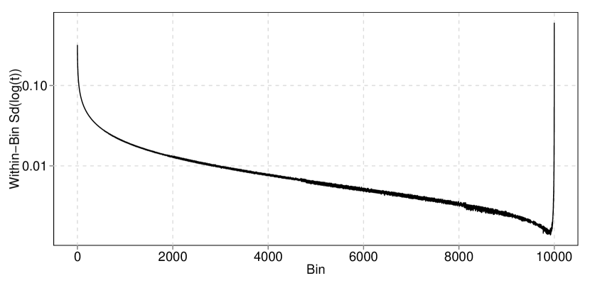
Figure 2. Within-bin range of $t$, measured by $\mbox{Sd}\left(\log t\right)$ in each bin, plotted on the log scale.

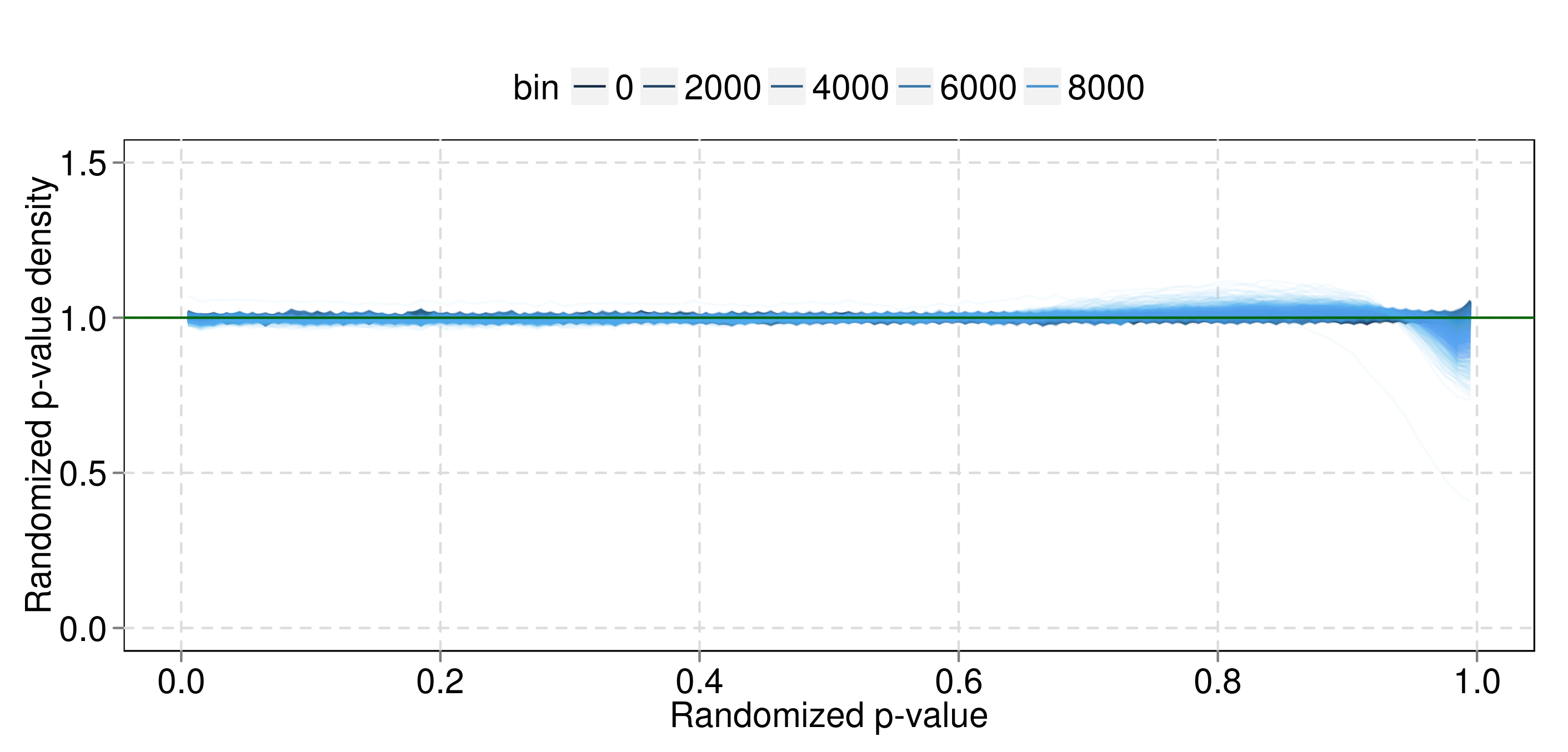
Figure 3. $p$-histogram densities for the marginal distribution within each bin. The densities are mostly flat, indicating that the $\hat{G}_{t}$ fit well.

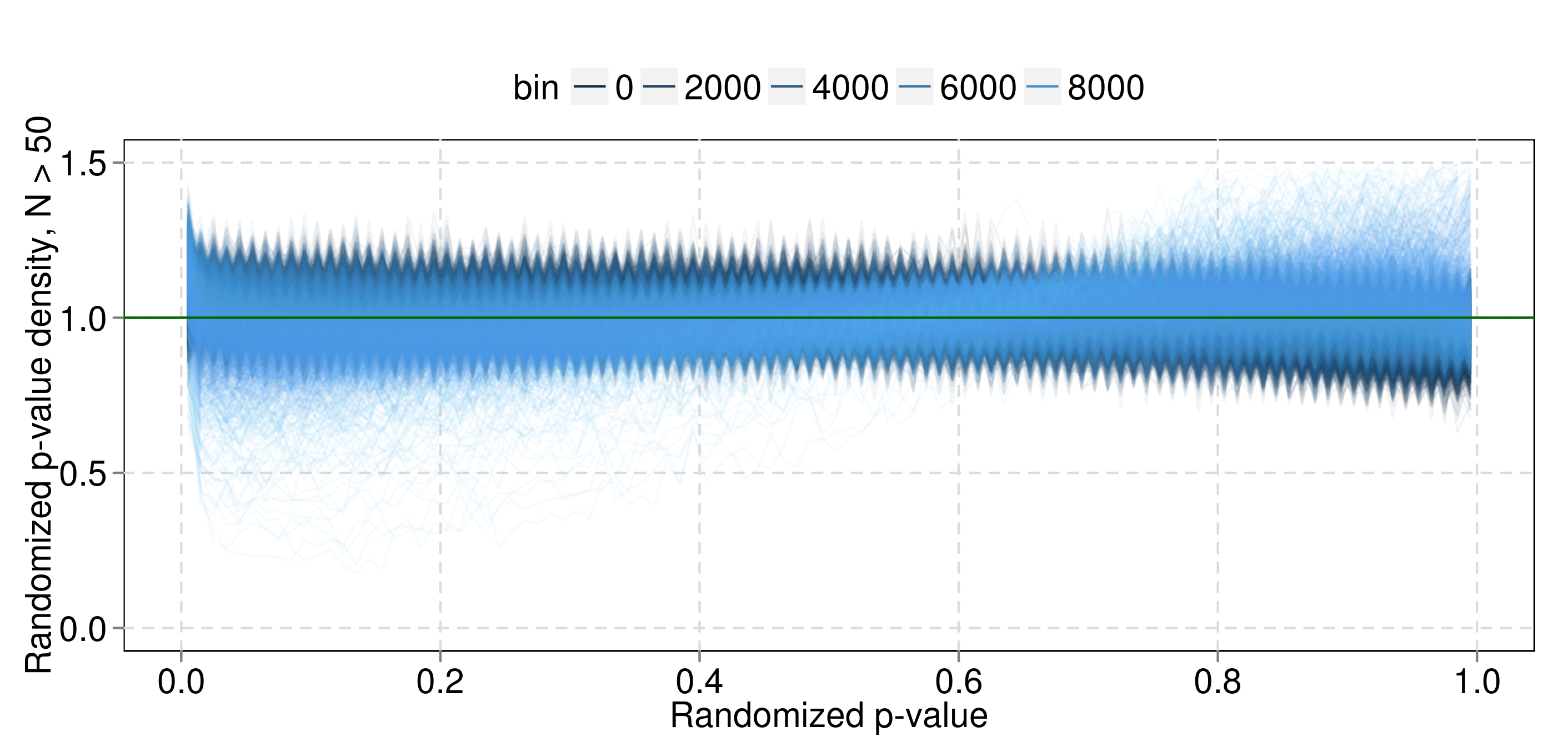
Figure 4. $p$-histogram densities for the marginal distribution within each bin, restricted to query-ad pairs with $N\geq 50$. The densities are mostly flat, indicating that the $\hat{G}_{t}$ fit well. The band is wider than the band in Figure 3 because we have fewer query-ad pairs, and so noisier histograms. The spikes are artifactual: they appear because we plot the histograms at discrete points, so we see the full range of the curves at those points and not in between.

Figure 5 shows the fitted $\mathrm{E}_{\hat{G}}\left(\theta\!\!\bigm{|}\!\!t\right)$, $\mathrm{Var}_{\hat{G}}\left(\theta\!\!\bigm{|}\!\!t\right)$ as functions of $t$. The $\mathrm{E}_{\hat{G}}\left(\theta\!\!\bigm{|}\!\!t\right)$, $\mathrm{Var}_{\hat{G}}\left(\theta\!\!\bigm{|}\!\!t\right)$ curves are nicely behaved, but the variance is noisy. We smoothed the curves and adjusted the $\hat{G}_{t}$ accordingly (we actually smoothed $\mathrm{E}_{\hat{G}}\left(\log\theta\!\!\bigm{|}\!\!t\right)$, $\mathrm{Var}_{\hat{G}}\left(\log\theta\!\!\bigm{|}\!\!t\right)$ to make sure the $\hat{G}_{t}$ stayed positive). Figure 6 shows the adjusted $\hat{G}_{t}$. We used the adjusted $\hat{G}_{t}$ to get $\hat{\mathrm{E}}\left(\theta\!\!\bigm{|}\!\!t\right)$, $\hat{\mathrm{Var}}\left(\theta\!\!\bigm{|}\!\!t\right)$, $\hat{\mathrm{E}}\left(\theta\!\!\bigm{|}\!\!t,y\right)$ and $\hat{\mathrm{Var}}\left(\theta\!\!\bigm{|}\!\!t,y\right)$, where

$$\hat{\mathrm{E}}\left(\theta\!\!\bigm{|}\!\!t\right)=\mathrm{E}_{\tilde{G_{t}}}\left(\theta\!\!\bigm{|}\!\!t\right)$$

and $\tilde{G_{t}}$ are the adjusted $G_{t}$ (the other expectations and variances are defined similarly). Figure 7 shows $\hat{G}_{t}$ for the middle bin, along with $y/N$ for the query-ad pairs with $N\geq 50$. $\hat{G}_{t}$ is centered at about the center of the $y/N$ histogram, but is narrower and smoother. The $y/N$ histogram also has a big spike at $0$. The marginal $p$-histograms fit well, indicating that while $\hat{G}_{t}$ does not have any mass at $0$, it captures this spike when we add Poisson noise to get the distribution of $y$.

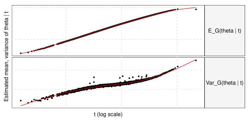
Figure 5. Unsmoothed (dots) and smoothed (red lines) $\mathrm{E}_{\hat{G}}\left(\theta\!\!\bigm{|}\!\!t\right)$ and $\mathrm{Var}_{\hat{G}}\left(\theta\!\!\bigm{|}\!\!t\right)$ (top and bottom, respectively). $\mathrm{E}_{\hat{G}}\left(\theta\!\!\bigm{|}\!\!t\right)$ is pretty smooth, but $\mathrm{Var}_{\hat{G}}\left(\theta\!\!\bigm{|}\!\!t\right)$ needs smoothing.

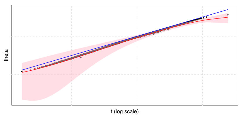
Figure 6. Adjusted $\hat{G}_{t}$. The black dots are an overall estimate of the mean $\theta$ in each bin ($\sum y/\sum N$). The blue line is $\theta=t$. The red line is the fitted $\mathrm{E}_{\hat{G}}\left(\theta\!\!\bigm{|}\!\!t\right)$, and the pink shaded area shows the $10$th to $95$th percentile of $\hat{G}_{t}$ at each $t$. The red curve is a little below the black dots because the smoothing pulls it down (Figure 5; the rightmost point has disproportionate leverage) , and because it is estimating $\mathrm{E}\left(\theta\right)=\mathrm{E}\left(y/N\right)$, which can be lower than $\sum y/\sum N=\sum\left(\frac{N}{\sum N}\right)\frac{y}{N}$ if bigger $N$s are associated with bigger $\theta$s. The likelihood improvement in Figure 8 suggests that this is a better shrinkage target.

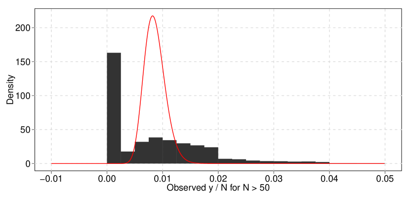
Figure 7. $\hat{G}_{t}$ (red) and $y/N$ histogram for pairs with $N\geq 50$ in the middle bin. Note that the histogram and the red distribution are not supposed to agree: the histogram is the red distribution, plus Poisson noise.

Evaluating these estimates is tricky since we do not know the true CTRs. We cannot directly measure how well the point estimates match $\theta$, or check that $\hat{\mathrm{Var}}\left(\theta\!\!\bigm{|}\!\!t,y\right)$ accurately estimates the distance between $\theta$ and $\mathrm{E}\left(\theta\!\!\bigm{|}\!\!t,y\right).$ Instead, we evaluate our estimates by using them to make predictions and predictive intervals. We randomly divided the impressions for each query-ad pair into training ($90\%$) and test ($10\%$) sets, and tried to predict the test data using the training data.

Second order calibration significantly improves our point estimates. We judged the point estimates $t$, $\mathrm{E}\left(\theta\!\!\bigm{|}\!\!t\right)$ and $\mathrm{E}\left(\theta\!\!\bigm{|}\!\!t,y\right)$ by their test set likelihood (under the assumed Poisson noise). Figure 8 shows the improvement in test set likelihood for each bin. Both ordinary and second order calibration increase test set likelihood in each bin, and help more as we move away from the center. Overall, using $\mathrm{E}\left(\theta\!\!\bigm{|}\!\!t\right)$, the ordinary calibration estimate, instead of $t$ increases the test set likelihood by $0.32\%$, and using the second order calibration estimate $\mathrm{E}\left(\theta\!\!\bigm{|}\!\!t,y\right)$ increases the test set likelihood by $0.63\%$. This is a substantial increase, given the difficulty of CTR estimation and the degree to which $t$ has been optimized. For comparison, using a constant, naive estimate for all items (the average CTR in the middle bin) gives a a test set likelihood $13.6\%$ lower than $t$.

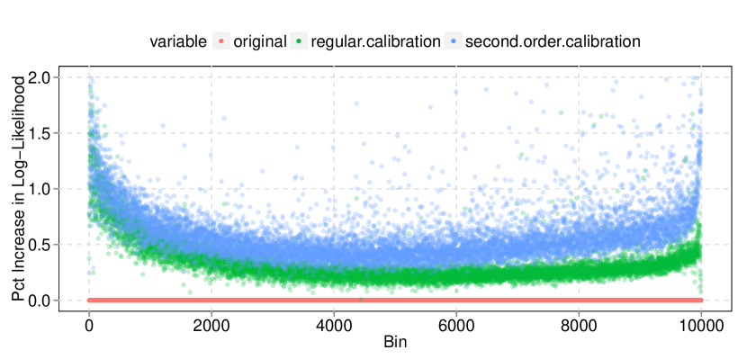
Figure 8. Percentage improvement in test set log-likelihood for $\mathrm{E}\left(\theta\!\!\bigm{|}\!\!t\right)$ (green) and $\mathrm{E}\left(\theta\!\!\bigm{|}\!\!t,y\right)$ (blue) over $t$ (red baseline).

We used the fit of the predictive distributions to judge the accuracy of $\hat{\mathrm{Var}}\left(\theta\!\!\bigm{|}\!\!t,y\right)$. The predictive distributions are wider when $\hat{\mathrm{Var}}\left(\theta\!\!\bigm{|}\!\!t,y\right)$ is large and shorter when $\hat{\mathrm{Var}}\left(\theta\!\!\bigm{|}\!\!t,y\right)$ is small, so if the predictive distributions match the data, $\hat{\mathrm{Var}}\left(\theta\!\!\bigm{|}\!\!t,y\right)$ is probably measuring uncertainty well. We assessed the fit of the predictive distributions with $p$-histograms like the one we used to check the fit of the marginal distribution. Figures 9 and 10 show that the predictive distributions fit well, both on the all the query-ad pairs, and those with $N\geq 25$ in the test set. The fit suggests that our $\mathrm{Var}\left(\theta\!\!\bigm{|}\!\!t,y\right)$ estimates are accurate enough to be useful.

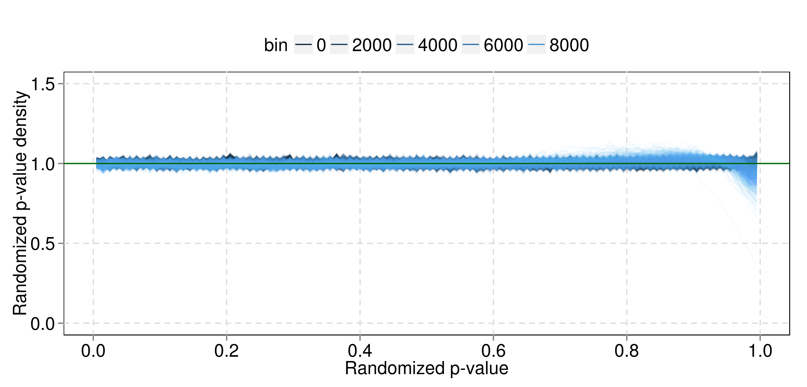
Figure 9. $p$-histogram densities for the predictive distribution within each bin. The densities are mostly flat, indicating that our predictive distributions mostly fit the test data.

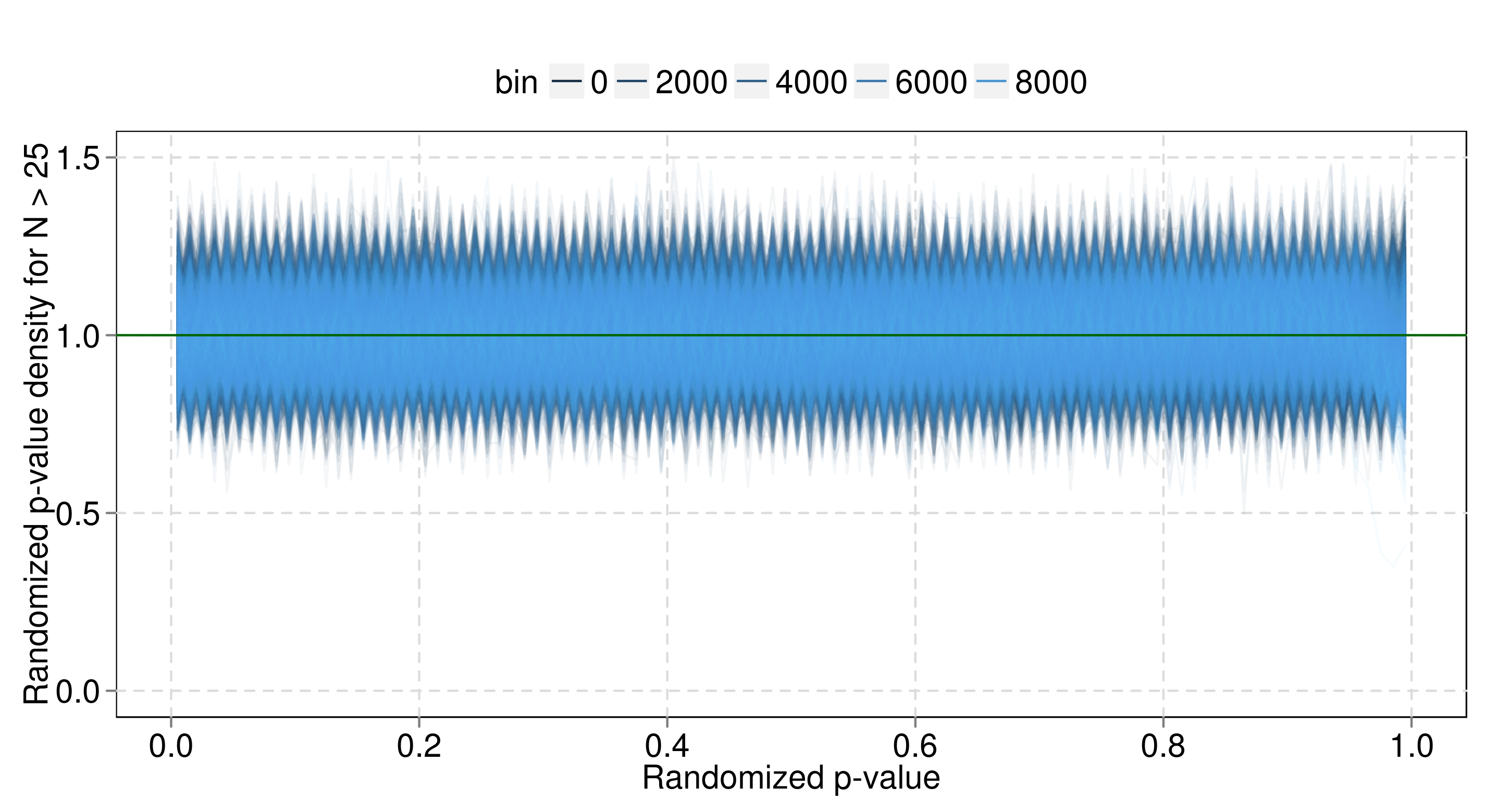
Figure 10. $p$-histogram densities for the predictive distribution within each bin, restricted to query-ad pairs with $N\geq 25$ in the test set. The densities are mostly flat, indicating that our predictive distributions mostly fit the test data.

The fit of our point estimates and predictive distributions also suggests that our Poisson model is approximately correct. To get the predictive distributions right, we need to divide the variance of $y\!\!\bigm{|}\!\!t$ into signal ($\mathrm{Var}\left(\theta\!\!\bigm{|}\!\!t\right)$) and noise ($y\!\!\bigm{|}\!\!\theta$). If we underestimate the noise, for example, our estimate for $\mathrm{Var}\left(\theta\!\!\bigm{|}\!\!t\right)$ will be too high. This means we will undershrink - our point estimates and will be too close to $y/N$, and our predictive distributions will be mis-centered. The fit of our predictive distributions indicates that our model is putting about the right weight on signal and noise.

Second order calibration gives us some interesting model-dependent estimates of performance. For example, we can use the model to estimate the fraction of the variance of $\theta$ explained by $t$:

$$\hat{R}^{2}=1-\frac{\hat{\mathrm{Var}}\left(\theta\!\!\bigm{|}\!\!t\right)}{\hat{\mathrm{Var}}\left(\theta\right)}$$

where

$$\hat{\mathrm{Var}}\left(\theta\right)=\mathrm{Var}\left[\hat{\mathrm{E}}\left(\theta\!\!\bigm{|}\!\!t\right)\right]+\mathrm{E}\left[\hat{\mathrm{Var}}\left(\theta\!\!\bigm{|}\!\!t\right)\right]$$

is the overall variance of $\theta$, estimated using the conditional variance formula and the fitted mean and variance of $\theta$ in each bin. For the CTR data, $\hat{R}^{2}$ was around $0.9$, indicating that $t$ is a strong predictor of $\theta$. We could use $\hat{R}^{2}$ to compare different candidates for $t$ (Amini and Johnson (2009) use a similar metric based on a random effects model). We can also use the model to estimate how much second order calibration lowers the variance in our estimate of $\theta$. Figure 11 plots $\mathrm{E}\left(\hat{\mathrm{Var}}\left(\theta\!\!\bigm{|}\!\!t,y\right)\right)/\hat{\mathrm{Var}}\left(\theta\!\!\bigm{|}\!\!t\right)$ for each bin, where the expectation is weighted by $N$ in the test set. Averaged over bins, this ratio was about $73\%$, which says that second order calibration gives us a mean squared error about $27\%$ less than ordinary calibration. The figure shows that the variance reduction is biggest in the high-$t$ bins; this makes sense, since query-ad pairs in those bins have more clicks, and thus more information about $\theta$. Although these performance estimates are model-dependent, and could be wrong because of model misspecification, the fit and predictive distribution checks above mean that the estimates are trustworthy enough to be interesting.

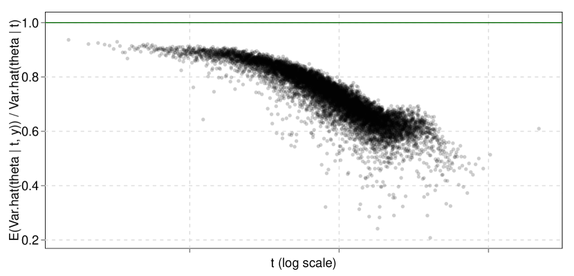
Figure 11. Plot of $\mathrm{E}\left(\hat{\mathrm{Var}}\left(\theta\!\!\bigm{|}\!\!t,y\right)\right)/\hat{\mathrm{Var}}\left(\theta\!\!\bigm{|}\!\!t\right)$ for each $t$ bin. The drop in variance is biggest in the high-$t$ bins, since query-ad pairs in those bins have more clicks and thus more information.

5.2. Simulated CTR data

Next, we tested our method on simulated CTR data that was based on our real data set. We used the same $N$ and $t$, generated true $\theta$ lognormally around $t$ with some bias and variance, and generated new clicks:

$$\log\theta_{i} \sim \mathcal{N}\left(\log t_{i}+\delta,\sigma^{2}\right)$$

$$y_{i} \sim \mathrm{Poisson}\left(N_{i}\lambda_{i}\right).$$

We used the same fitting method as for real data (so we had around 2-3 billion query-ad pairs), and looked at the results for different values of $\delta$ and $\sigma$. To make computation easier, we used every tenth bin instead of every bin.

Figure 12 shows that a Gamma model for $G_{t}$ fit the simulated data reasonably well - not surprising, since the Gamma distribution approximates the lognormal distribution well when $\sigma$ is small. The Gamma model doesn’t quite fit the data when $\sigma$ is large. We smoothed as before and calculated $\hat{\mathrm{E}}\left(\theta\!\!\bigm{|}\!\!t\right)$, $\hat{\mathrm{Var}}\left(\theta\!\!\bigm{|}\!\!t\right)$, $\hat{\mathrm{E}}\left(\theta\!\!\bigm{|}\!\!t,y\right)$ and $\hat{\mathrm{Var}}\left(\theta\!\!\bigm{|}\!\!t,y\right)$.

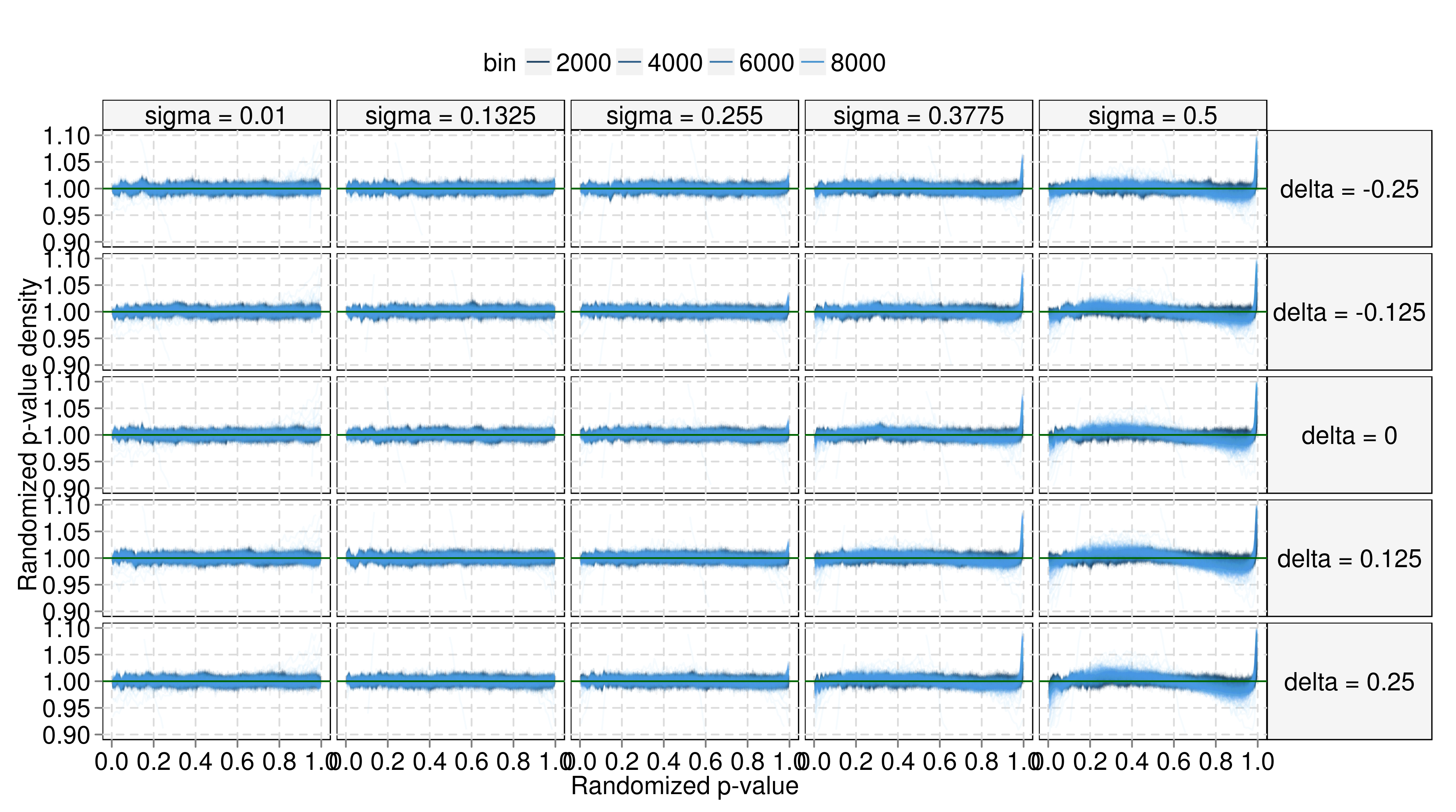
Figure 12. $p$-histogram densities for the marginal distribution within each bin. The panels from show increasing $\sigma$ (top to bottom) and $\delta$ (left to right).

Our estimates are accurate for all the values of $\delta$ and $\sigma$ that we tried. We measured their accuracy directly, since we knew the true $\theta\!\!\bigm{|}\!\!t$ distributions. Figure 13 shows that our estimates of $\mathrm{E}\left(\theta\!\!\bigm{|}\!\!t\right)$, $\mathrm{Var}\left(\theta\!\!\bigm{|}\!\!t\right)$, $\mathrm{E}\left(\theta\!\!\bigm{|}\!\!t,y\right)$ and $\mathrm{Var}\left(\theta\!\!\bigm{|}\!\!t,y\right)$ were close to the corresponding true quantities. Calculating posterior quantities in the true lognormal-Poisson model is computationally expensive, so we found $\mathrm{E}\left(\theta\!\!\bigm{|}\!\!t,y\right)$ and $\mathrm{Var}\left(\theta\!\!\bigm{|}\!\!t,y\right)$ by approximating the lognormal with a Gamma distribution. This worked better than approximation with a grid of point masses, and yielded an accurate approximation for $\mathrm{E}\left(\theta\!\!\bigm{|}\!\!t,y\right)$, but cannot capture the heavy tails of the lognormal distribution and slightly underestimated $\mathrm{Var}\left(\theta\!\!\bigm{|}\!\!t,y\right)$.

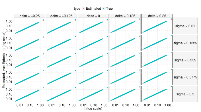
(a) $\mathrm{E}\left(\theta\!\!\bigm{|}\!\!t\right)$ and $\hat{\mathrm{E}}\left(\theta\!\!\bigm{|}\!\!t\right)$ as functions of $t$.

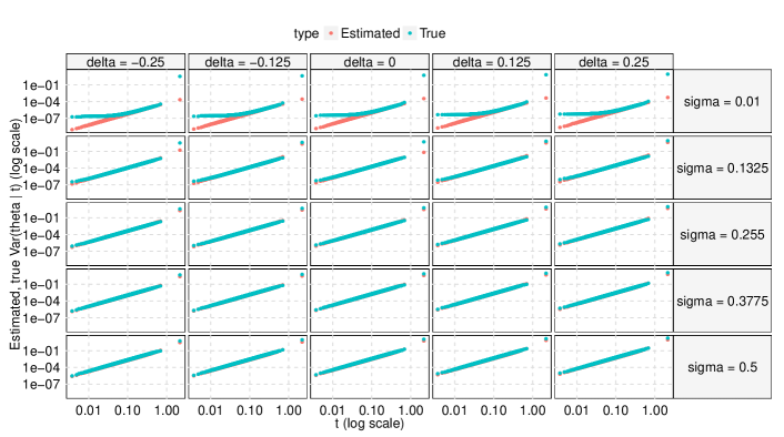
(b) $\mathrm{Var}\left(\theta\!\!\bigm{|}\!\!t\right)$ and $\hat{\mathrm{Var}}\left(\theta\!\!\bigm{|}\!\!t\right)$ as functions of $t$.

Figure 13. Accuracy plots for $\mathrm{E}\left(\theta\!\!\bigm{|}\!\!t\right)$, $\mathrm{Var}\left(\theta\!\!\bigm{|}\!\!t\right)$, $\mathrm{E}\left(\theta\!\!\bigm{|}\!\!t,y\right)$ and $\mathrm{Var}\left(\theta\!\!\bigm{|}\!\!t,y\right)$. For the first two, we plot the estimates and the true quantities. For the second two, we plot the in-bin mean-squared-error between the estimate and true quantities, scaled by $\mathrm{E}\left(\theta\!\!\bigm{|}\!\!t\right)$ to put the different bins on the same scale. In each plot the panels show increasing $\sigma$ (top to bottom) and $\delta$ (left to right). Within each panel, each dot is a $t$-bin. All the estimated quantities are pretty close to the true quantities.

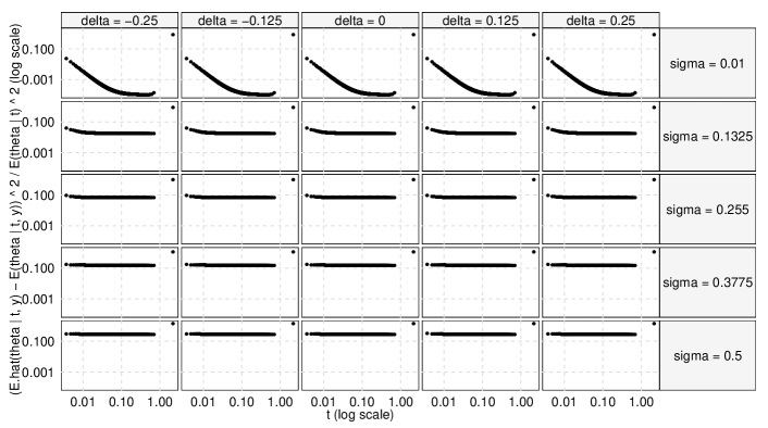
(c) In-bin average $\left(\mathrm{E}\left(\theta\!\!\bigm{|}\!\!t,y\right)-\hat{\mathrm{E}}\left(\theta\!\!\bigm{|}\!\!t,y\right)\right)^{2}/\mathrm{E}\left(\theta\!\!\bigm{|}\!\!t\right)^{2}$.

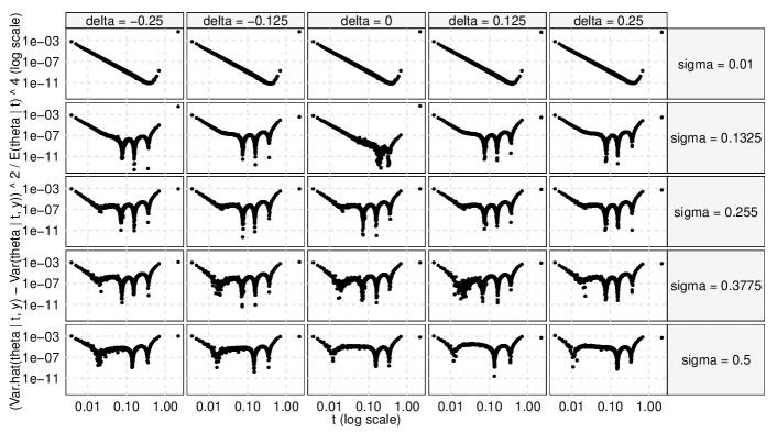
(d) In-bin average $\left(\mathrm{Var}\left(\theta\!\!\bigm{|}\!\!t,y\right)-\hat{\mathrm{Var}}\left(\theta\!\!\bigm{|}\!\!t,y\right)\right)^{2}/\mathrm{E}\left(\theta\!\!\bigm{|}\!\!t\right)^{4}$.

Figure 13. (continued from previous page)

Figure 14 shows if this were a real problem, second order calibration would not be perfect, but would be good enough to be useful. It gives better point estimates - $\hat{\mathrm{E}}\left(\theta\!\!\bigm{|}\!\!t,y\right)$ substantially improves on $t$, $\hat{\mathrm{E}}\left(\theta\!\!\bigm{|}\!\!t\right)$, and $\mathrm{E}\left(\theta\!\!\bigm{|}\!\!t\right)$, and estimates $\theta$ almost as well as our approximate $\mathrm{E}\left(\theta\!\!\bigm{|}\!\!t,y\right)$. The improvement is especially large when $\sigma$ is big, since the bigger $\sigma$ is, the more information is item-specific, and the more we can gain by using it. Our variance estimates are also reasonably accurate. On average, $\hat{\mathrm{Var}}\left(\theta\!\!\bigm{|}\!\!t\right)$ is usually close to $\left(\hat{E}\left(\theta\!\!\bigm{|}\!\!t\right)-\theta\right)^{2}$, but is about $5-10\%$ too small (Figure 15). This is because the true distribution of $\theta\!\!\bigm{|}\!\!t$ is lognormal, and our Gamma model cannot capture its heavy tails. Our $p$-histograms detect this misfit when $\sigma$ is large, but are not sensitive enough to detect the misfit when $\sigma$ is small.

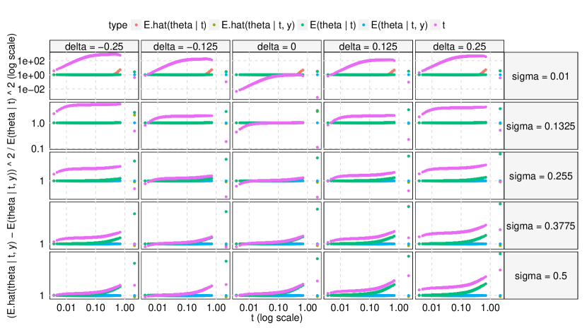
Figure 14. In-bin mean-squared error, relative to the (approximated) $\mathrm{E}\left(\theta\!\!\bigm{|}\!\!t,y\right)$. The perfect estimator $\mathrm{E}\left(\theta\!\!\bigm{|}\!\!t,y\right)$ has a relative error of $1$. $\hat{\mathrm{E}}\left(\theta\!\!\bigm{|}\!\!t,y\right)$ almost always has relative error very close to $1$, so it is almost as good as $\mathrm{E}\left(\theta\!\!\bigm{|}\!\!t,y\right)$. $\mathrm{E}\left(\theta\!\!\bigm{|}\!\!t\right)$ and $\hat{\mathrm{E}}\left(\theta\!\!\bigm{|}\!\!t\right)$ are very close, and perform worse than $\mathrm{E}\left(\theta\!\!\bigm{|}\!\!t,y\right)$ when $\sigma$ is large. $t$ does badly, but actually outperforms $\mathrm{E}\left(\theta\!\!\bigm{|}\!\!t,y\right)$ when $\sigma$ and $\delta$ are both small - in that case, $\theta\approx t$, so $t$ is better than $\mathrm{E}\left(\theta\!\!\bigm{|}\!\!t,y\right)$, which only uses $t$ through the bin.

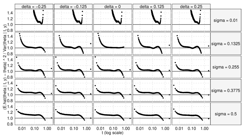
Figure 15. In-bin averages of $\left(\hat{\mathrm{E}}\left(\theta\!\!\bigm{|}\!\!t,y\right)-\theta\right)^{2}/\hat{\mathrm{Var}}\left(\theta\!\!\bigm{|}\!\!t,y\right)$. If our estimates were perfect, these would be $1$. Except when $\sigma$ is small, the ratios are close to $1$, but $5-10\%$ too high. This indicates $\hat{\mathrm{Var}}\left(\theta\!\!\bigm{|}\!\!t,y\right)$ is underestimating the error of $\hat{\mathrm{E}}\left(\theta\!\!\bigm{|}\!\!t,y\right)$; our Gamma model cannot capture the heavy lognormal tails of the true $\theta\!\!\bigm{|}\!\!t$ distribution.

5.3. Simulated Normal data

As a final illustration of our method, we consider a smaller simulated normal data set with $10$ million items. Each item had a covariate $\boldsymbol{x}\in\mathbb{R}^{10}$ with iid $\mathcal{N}\left(0,1\right)$ entries, and a response $y\sim\mathcal{N}\left(\theta,1\right)$. $\theta$ was a quadratic function of $\boldsymbol{x}$, plus noise:

$$\theta=\boldsymbol{x}^{\prime}\beta+\left(\boldsymbol{x}^{\prime}\gamma\right)^{2}+\varepsilon,$$

where $\varepsilon$ were drawn iid from a Laplace distribution with variance $2$. The coefficient vectors $\beta$ and $\gamma$ each had entries that were $0$ with probability $0.95$ and $\mathcal{N}\left(0,1\right)$ ($\mathcal{N}\left(0,0.1^{2}\right)$ for $\gamma$) with probability $0.05$. To get $t$, we divided the data into five folds and regressed $y$ onto $\boldsymbol{x}$ (with no interactions or quadratic terms). Finally, we fit $G_{t}$ using a seven-component normal mixture (using the R package “mixfdr” (Muralidharan, 2010)), and smoothed $\hat{\mathrm{E}}\left(\theta\!\!\bigm{|}\!\!t\right)$ and $\hat{\mathrm{Var}}$$\left(\theta\!\!\bigm{|}\!\!t\right)$.

Figure 16 shows the $p$-histograms for our fitted model. Although the fit is decent in the center of the distribution, we see many more low and high $p$s than our fitted $y\!\!\bigm{|}\!\!t$ densities predict. Our normal mixture model does not capture the heavy tails of the distribution of $\theta\!\!\bigm{|}\!\!t$. If this were a real data set, the $p$-histograms would tell us our model for $G_{t}$ doesn’t fit, and we would refine it.

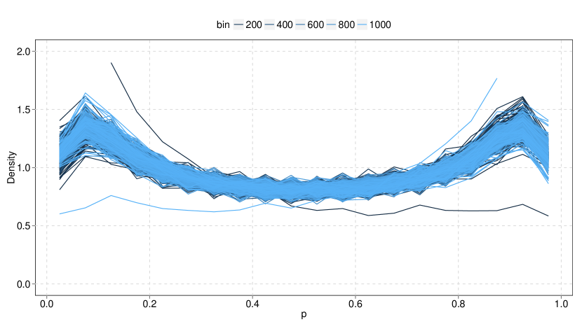
Figure 16. Marginal $p$-histograms for normal data. The “smile” indicates that our model gives a light-tailed estimate for the distribution of $y\!\!\bigm{|}\!\!t$. The left- and rightmost bins are miscentered as well.

It is interesting, though, to see how our flawed model performs. Figure 17 shows that $\hat{\mathrm{E}}\left(\theta\!\!\bigm{|}\!\!t,y\right)$ is a good, but not perfect point estimate. It estimates $\theta$ much more accurately than $t$ or $y$, and is about $11\%$ worse than $\mathrm{E}\left(\theta\!\!\bigm{|}\!\!t,y\right)$ (calculated using a fine grid approximation). Figure 18 shows that our light-tailed fit makes our variance estimates too small - $\hat{\mathrm{E}}\left(\theta\!\!\bigm{|}\!\!t,y\right)$ is, on average, about $72\%$ further from $\theta$ than $\hat{\mathrm{Var}}\left(\theta\!\!\bigm{|}\!\!t,y\right)$ indicates. Theorem 1 says that a better-fitting model should perform better.

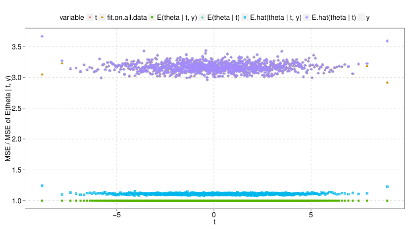
Figure 17. Mean squared error of the different estimators, relative to the mean squared error of $\mathrm{E}\left(\theta\!\!\bigm{|}\!\!t,y\right)$. $t$, a regression on all the data (instead of dividing into folds), $\mathrm{E}\left(\theta\!\!\bigm{|}\!\!t\right)$ and $\hat{\mathrm{E}}\left(\theta\!\!\bigm{|}\!\!t\right)$ all perform very similarly - their points are superimposed. $\hat{\mathrm{E}}\left(\theta\!\!\bigm{|}\!\!t,y\right)$ (light blue) is about $11\%$ worse than $\mathrm{E}\left(\theta\!\!\bigm{|}\!\!t,y\right)$.

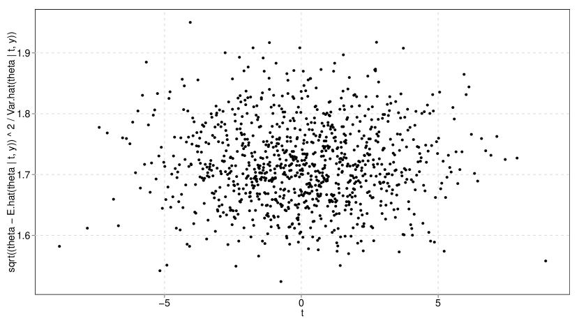
Figure 18. Square roots of the within-bin averages of $\left(\hat{\mathrm{E}}\left(\theta\!\!\bigm{|}\!\!t,y\right)-\theta\right)^{2}/\hat{\mathrm{Var}}\left(\theta\!\!\bigm{|}\!\!t,y\right)$. On average, $\hat{\mathrm{E}}\left(\theta\!\!\bigm{|}\!\!t,y\right)$ is about $72\%$ further from $\theta$ than $\hat{\mbox{Sd}}\left(\theta\!\!\bigm{|}\!\!t,y\right)$.

6. Summary

This paper considers second order calibration, a simple way to get approximate posteriors from the output of an arbitrary black box estimation method. The idea, which extends the usual idea of calibrating the mean, is to approximate the distribution of $\theta\!\!\bigm{|}\!\!\boldsymbol{x}$ with the distribution $\theta\!\!\bigm{|}\!\!t$, and estimate the latter distribution using the data. We give a five step procedure to estimate these quantities: bin by $t$, estimate the distribution of $\theta\!\!\bigm{|}\!\!t$ in each bin, collect and if necessary smooth the estimates across bins, check the fit, and use the estimates to calculate $\hat{\mathrm{E}}\left(\theta\!\!\bigm{|}\!\!t\right)$, $\hat{\mathrm{Var}}\left(\theta\!\!\bigm{|}\!\!t\right)$, $\hat{\mathrm{E}}\left(\theta\!\!\bigm{|}\!\!t,y\right)$ and $\hat{\mathrm{Var}}\left(\theta\!\!\bigm{|}\!\!t,y\right)$. This is a reasonable thing to do: if the distribution of $y\!\!\bigm{|}\!\!\theta$ is Poisson or a continuous natural exponential family, the data has enough information to estimate $\mathrm{E}\left(\theta\!\!\bigm{|}\!\!t\right)$, $\mathrm{Var}\left(\theta\!\!\bigm{|}\!\!t\right)$, $\mathrm{E}\left(\theta\!\!\bigm{|}\!\!t,y\right)$ and $\mathrm{Var}\left(\theta\!\!\bigm{|}\!\!t,y\right)$ effectively. When applied to real and simulated data, second order calibration improves point estimates and gives useful accuracy estimates.

6.1. Acknowledgements

We thank many colleagues for helpful comments, suggestions and discussion: Sugato Basu, Nick Chamandy, Brad Efron, Brendan McMahan, Donal McMahon, Deirdre O’Brien, Daryl Pregibon and Tom Zhang.

Appendix A Proofs

From now on, we work within a bin. We always condition on $t$ (assumed constant in the bin), so we drop it to simplify notation.

A.1. Posterior Cumulant Formulas

In Section 4, we stated Robbins’ formulas for the posterior mean and variance of $\theta$ when $f_{\theta}$ is $\mathrm{Poisson}\left(N\theta\right)$. Similar formulas exist for higher moments. Using Robbins’ argument, it is easy to show that

(2) $$\mathrm{E}\left(\theta^{k}\!\!\bigm{|}\!\!y\right)=\frac{\left[y\right]_{k}}{N^{k}}+\frac{1}{N^{k}}\frac{\Delta_{G}\left(y\right)}{f_{G}\left(y\right)}$$

where $\left[y\right]_{k}=y\left(y-1\right)\ldots\left(y-k+1\right)$, and $\Delta\left(y\right)=f_{G}\left(y+k\right)\left[y+k\right]_{k}-f_{G}\left(y\right)\left[y\right]_{k}$. The two terms in the formula have a natural interpretation. The uniformly minimum variance unbiased (UMVU) estimate of $\theta^{k}$ is $\left[y\right]_{k}/N^{k}$, so the first term in the formula is the UMVU estimate of $\theta^{k}$. The second term is a correction that depends on the prior.

When $f_{\theta}$ is a continuous natural exponential family, it is easier to work with cumulants than with moments. Let $\kappa_{k}$ be the $k$th cumulant of a distribution and let $p_{k}$ be the polynomial that expresses the $k$th cumulant of a distribution in terms of the first $k$ moments, so that for any distribution,

$$\kappa_{k}=p_{k}\left(\mu_{1},\ldots,\mu_{k}\right)$$

where $\mu_{j}$ is the $j$th moments. Let $\kappa_{k}\left(\theta\!\!\bigm{|}\!\!y\right)$ be the $k$th posterior cumulant of the $\theta\!\!\bigm{|}\!\!y$ distribution (it depends on $G$, but we suppress this). Simple algebra shows that if $f_{\theta}$ is a continuous natural exponential family with base density $f_{0}$, then

(3) $$\kappa_{k}\left(\theta\!\!\bigm{|}\!\!y\right)=p_{k}\left(\frac{f_{0}^{\prime}\left(y\right)}{f_{0}\left(y\right)},\ldots,\left(-1\right)^{k}\frac{f_{0}^{\left(k\right)}\left(y\right)}{f_{0}\left(y\right)}\right)+p_{k}\left(\frac{f_{G}^{\prime}\left(y\right)}{f_{G}\left(y\right)},\ldots,\frac{f_{G}^{\left(k\right)}\left(y\right)}{f_{G}\left(y\right)}\right).$$

The two terms in this formula have the same interpretation as the two terms in equation 2. The UMVU estimator of $\theta^{i}$ is $\left(-1\right)^{i}\frac{f_{0}^{\left(i\right)}}{f_{0}}$ (Sharma, 1973), so the first term plugs UMVU estimates of $\theta,\ldots,\theta^{k}$ into $p_{k}$ to estimate $\kappa_{k}$. The second term is a correction that depends on the prior.

A.2. Regularized Cumulant Estimators

Equations 2 and 3 divide by $f_{G}\left(y\right)$. If our estimate $\hat{G}$ gives a light-tailed $f_{\hat{G}}$, this division can make our posterior moment and cumulant estimates behave badly. To avoid this, we follow the approach of Zhang (1997) and regularize our estimates: instead of divding by $f_{\hat{G}}$, we divide by $\max\left(f_{\hat{G}},\rho\right)$, where $\rho$ is a tuning parameter. This gives regularized estimators

$$\hat{\mathrm{E}}_{\rho}\left(\theta^{k}\!\!\bigm{|}\!\!y\right) = \frac{\left[y\right]_{k}}{N^{k}}+\frac{1}{N^{k}}\frac{\Delta_{\hat{G}}\left(y\right)}{\max\left(f_{\hat{G}}\left(y\right),\rho\right)}$$

$$\hat{\kappa}_{k,\rho}\left(\theta\!\!\bigm{|}\!\!y\right) = p_{k}\left(\frac{f_{0}^{\prime}\left(y\right)}{f_{0}\left(y\right)},\ldots,\left(-1\right)^{k}\frac{f_{0}^{\left(k\right)}\left(y\right)}{f_{0}\left(y\right)}\right)+p_{k}\left(\frac{f_{\hat{G}}^{\prime}\left(y\right)}{\max\left(f_{\hat{G}}\left(y\right),\rho\right)},\ldots,\frac{f_{\hat{G}}^{\left(k\right)}\left(y\right)}{\max\left(f_{\hat{G}}\left(y\right),\rho\right)}\right)$$

instead of our original, unregularized estimators $\hat{\mathrm{E}}\left(\theta^{k}\!\!\bigm{|}\!\!y\right)$, $\hat{\kappa}_{k}\left(\theta\!\!\bigm{|}\!\!y\right)$.

These regularized estimators guard against overshrinking. In the far tail, the second term in each formula tends to zero, since $\max\left(f_{\hat{G}},\rho\right)$ becomes $\rho$ and the numerator of each ratio tends to zero. That means that the correction term that depends on the prior disappears, and our estimates reduce to frequentist estimators. This makes sense: we don’t know much about the prior in the far tail, so we shouldn’t deviate too much from the safe frequentist estimator. The regularized estimators are similar in this respect to the limited translation estimators introduced by Efron and Morris (1971).

A.3. Proof of Theorem 1

We prove Theorem 1 by bounding the error in estimating the posterior cumulants and moments in terms of the error in estimating the marginal density. We first bound the error of the regularized estimates, then use those bounds that to bound the error of the unregularized estimates.

Lemma 1.

The regularized Poisson moment estimator has error at most

$$\left\|\hat{\mathrm{E}}_{\rho}\left(\theta^{k}\!\!\bigm{|}\!\!y\right)-\mathrm{E}\left(\theta^{k}\!\!\bigm{|}\!\!y\right)\right\|\leq\frac{C_{G,\rho}}{N^{k}}\left(\left\|\left(f_{\hat{G}}-f_{G}\right)^{2}\right\|^{\frac{1}{2}}+\left\|\left(f_{\hat{G}}\left(y+k\right)-f_{G}\left(y+k\right)\right)^{2}\right\|^{\frac{1}{2}}\right)+\frac{D_{G,\rho}}{N^{k}}$$

where $C_{G,\rho}$, $D_{G,\rho}$ only depend on $G$ and $\rho$: $C_{G,\rho}=\frac{1}{\rho^{2}}\left\|\Delta_{G}^{2}\right\|^{\frac{1}{2}}+\frac{1}{\rho}\left\|\left[y\right]_{k}^{2}\right\|^{\frac{1}{2}}+\frac{1}{\rho}\left\|\left[y+k\right]_{k}^{2}\right\|^{\frac{1}{2}}$ and $D_{G,\rho}=\left\|\left(\frac{\Delta_{G}\left(y\right)}{f_{G}\left(y\right)}\right)\left(1-\frac{f_{G}\left(\rho\right)}{\rho}\right)_{+}\right\|$.

Proof.

We first bound $\left\|\hat{\mathrm{E}}_{\rho}\left(\theta^{k}\!\!\bigm{|}\!\!y\right)-\mathrm{E}\left(\theta^{k}\!\!\bigm{|}\!\!y\right)\right\|$:

$$\left\|\hat{\mathrm{E}}_{\rho}\left(\theta^{k}\!\!\bigm{|}\!\!y\right)-\mathrm{E}\left(\theta^{k}\!\!\bigm{|}\!\!y\right)\right\|\leq N^{-k}\left\|\left(\frac{\Delta_{\hat{G}}\left(y\right)}{f_{\hat{G}}\left(y\right)\vee\rho}-\frac{\Delta_{G}\left(y\right)}{f_{G}\left(y\right)\vee\rho}\right)\right\|+N^{-k}\left\|\left(\frac{\Delta_{G}\left(y\right)}{f_{G}\left(y\right)\vee\rho}-\frac{\Delta_{G}\left(y\right)}{f_{G}\left(y\right)}\right)\right\|$$

The second term is $D_{G,\rho}$. We bound the first term using Cauchy-Schwartz and the triangle inequality:

$$\left\|\left(\frac{\Delta_{\hat{G}}\left(y\right)}{f_{\hat{G}}\left(y\right)\vee\rho}-\frac{\Delta_{G}\left(y\right)}{f_{G}\left(y\right)\vee\rho}\right)\right\| \leq \left\|\frac{\Delta_{G}}{f_{G}\vee\rho}\left(\frac{f_{G}\vee\rho-f_{\hat{G}}\vee\rho}{f_{\hat{G}}\vee\rho}\right)\right\|+\left\|\left(\frac{\Delta_{G}-\Delta_{\hat{G}}}{f_{\hat{G}}\vee\rho}\right)\right\|$$

$$\leq \frac{1}{\rho^{2}}\left\|\Delta_{G}^{2}\right\|^{\frac{1}{2}}\left\|\left(f_{G}-f_{\hat{G}}\right)^{2}\right\|^{\frac{1}{2}}$$

$$+\frac{1}{\rho}\left\|\left[y\right]_{k}^{2}\right\|^{\frac{1}{2}}\left\|\left(f_{G}-f_{\hat{G}}\right)^{2}\right\|^{\frac{1}{2}}$$

$$+\frac{1}{\rho}\left\|\left[y+k\right]_{k}^{2}\right\|^{\frac{1}{2}}\left\|\left(f_{G}\left(y+k\right)-f_{\hat{G}}\left(y+k\right)\right)^{2}\right\|^{\frac{1}{2}}.$$

∎

Lemma 2.

The regularized posterior cumulant estimator for continuous natural exponential families has error at most

$$\left\|\hat{\kappa}_{k,\rho}\left(\theta\!\!\bigm{|}\!\!y\right)-\kappa_{k}\left(\theta\!\!\bigm{|}\!\!y\right)\right\| \leq C_{G,\hat{G},\rho}\left\|\left(\sum_{i=0}^{k}\left(f_{G}^{\left(i\right)}-f_{\hat{G}}^{\left(i\right)}\right)^{2}\right)^{\frac{1}{2}}\right\|$$

$$+\frac{1}{\rho}\left\|p_{k}\left(\frac{f_{G}^{\prime}}{f_{G}\vee\rho},\ldots,\frac{f_{G}^{\left(k\right)}}{f_{G}\vee\rho}\right)\right\|^{\frac{1}{2}}\left\|\left(f_{G}-f_{\hat{G}}\right)^{2}\right\|^{\frac{1}{2}}$$

$$+\left\|p_{k}\left(\frac{f_{G}^{\prime}}{f_{G}\vee\rho},\ldots,\frac{f_{G}^{\left(k\right)}}{f_{G}\vee\rho}\right)-p_{k}\left(\frac{f_{G}^{\prime}}{f_{G}},\ldots,\frac{f_{G}^{\left(k\right)}}{f_{G}}\right)\right\|$$

Proof.

We have

$$\left\|\hat{\kappa}_{k,\rho}\left(\theta\!\!\bigm{|}\!\!y\right)-\kappa_{k}\left(\theta\!\!\bigm{|}\!\!y\right)\right\| \leq \left\|p_{k}\left(\frac{f_{\hat{G}}^{\prime}}{f_{\hat{G}}\vee\rho},\ldots,\frac{f_{\hat{G}}^{\left(k\right)}}{f_{\hat{G}}\vee\rho}\right)-p_{k}\left(\frac{f_{G}^{\prime}}{f_{G}\vee\rho},\ldots,\frac{f_{G}^{\left(k\right)}}{f_{G}\vee\rho}\right)\right\|$$

$$+\left\|p_{k}\left(\frac{f_{G}^{\prime}}{f_{G}\vee\rho},\ldots,\frac{f_{G}^{\left(k\right)}}{f_{G}\vee\rho}\right)-p_{k}\left(\frac{f_{G}^{\prime}}{f_{G}},\ldots,\frac{f_{G}^{\left(k\right)}}{f_{G}}\right)\right\|.$$

To bound the first term, we write $p_{k}\left(\frac{f^{\prime}}{f},\ldots,\frac{f^{\left(k\right)}}{f}\right)=\frac{1}{f^{k}}H\left(f^{\prime},\ldots,f^{\left(k\right)}\right)$ where $H$ is a polynomial of degree $k$; we can do this since every term in $p_{k}$ has degree $k$. Let $B$ be the box $\prod_{i=1}^{k}\left[-\max\left(\left\|f_{G}^{\left(i\right)}\right\|_{\infty},\left\|f_{\hat{G}}^{\left(i\right)}\right\|_{\infty}\right),\max\left(\left\|f_{G}^{\left(i\right)}\right\|_{\infty},\left\|f_{\hat{G}}^{\left(o\right)}\right\|_{\infty}\right)\right]$, and let $C=\sup_{B}\left\|\nabla H\right\|_{2}$ be the maximum of the $\ell^{2}$ norm of the gradient over $B$. $C$ only depends on $G$, $\hat{G}$ through $\left\|f_{G}^{\left(i\right)}\right\|_{\infty}$ and $\left\|f_{\hat{G}}^{\left(i\right)}\right\|_{\infty}$. Then the first term is bounded by

$$\left\|\frac{1}{\left(f_{\hat{G}}\vee\rho\right)^{k}}H\left(f_{\hat{G}}^{\prime},\ldots,f_{\hat{G}}^{\left(k\right)}\right)-\frac{1}{\left(f_{G}\vee\rho\right)^{k}}H\left(f_{G}^{\prime},\ldots,f_{G}^{\left(k\right)}\right)\right\|$$

$$= \left\|\frac{1}{\left(f_{\hat{G}}\vee\rho\right)^{k}}H\left(f_{\hat{G}}^{\prime},\ldots,f_{\hat{G}}^{\left(k\right)}\right)-\frac{1}{\left(f_{G}\vee\rho\right)^{k}}H\left(f_{G}^{\prime},\ldots,f_{G}^{\left(k\right)}\right)\right\|$$

$$\leq \frac{1}{\rho^{k}}\left\|H\left(f_{\hat{G}}^{\prime},\ldots,f_{\hat{G}}^{\left(k\right)}\right)-H\left(f_{G}^{\prime},\ldots,f_{G}^{\left(k\right)}\right)\right\|+\frac{1}{\rho}\left\|\frac{H\left(f_{G}^{\prime},\ldots,f_{G}^{\left(k\right)}\right)}{\left(f_{G}\vee\rho\right)^{k}}\left(f_{G}\vee\rho-f_{\hat{G}}\vee\rho\right)\right\|$$

$$\leq \frac{C}{\rho^{k}}\left\|\left(\sum\left(f_{G}^{\left(i\right)}-f_{\hat{G}}^{\left(i\right)}\right)^{2}\right)^{\frac{1}{2}}\right\|+\frac{1}{\rho}\left\|\left(\frac{H\left(f_{G}^{\prime},\ldots,f_{G}^{\left(k\right)}\right)}{f_{G}^{k}}\right)^{2}\right\|^{\frac{1}{2}}\left\|\left(f_{G}-f_{\hat{G}}\right)^{2}\right\|^{\frac{1}{2}}$$

∎

Lemma 3.

The unregularized Poisson moment estimator has error at most

$$\left\|\hat{\mathrm{E}}\left(\theta^{k}\!\!\bigm{|}\!\!y\right)-\mathrm{E}\left(\theta^{k}\!\!\bigm{|}\!\!y\right)\right\|\leq N^{-k}\inf_{\rho}\left[C_{G,\rho}\left(\left\|\left(f_{\hat{G}}-f_{G}\right)^{2}\right\|^{\frac{1}{2}}+\left\|\left(f_{\hat{G}}\left(y+k\right)-f_{G}\left(y+k\right)\right)^{2}\right\|^{\frac{1}{2}}\right)+D_{G,\rho}+D_{\hat{G},\rho}\right]$$

Proof.

For any $\rho$,

$$\left\|\hat{\mathrm{E}}\left(\theta^{k}\!\!\bigm{|}\!\!y\right)-\mathrm{E}\left(\theta^{k}\!\!\bigm{|}\!\!y\right)\right\|\leq\left\|\hat{\mathrm{E}}_{\rho}\left(\theta^{k}\!\!\bigm{|}\!\!y\right)-\hat{\mathrm{E}}\left(\theta^{k}\!\!\bigm{|}\!\!y\right)\right\|+\left\|\hat{\mathrm{E}}_{\rho}\left(\theta^{k}\!\!\bigm{|}\!\!y\right)-\mathrm{E}\left(\theta^{k}\!\!\bigm{|}\!\!y\right)\right\|.$$

The first term is $N^{-k}D_{\hat{G},\rho}$, and we can bound the second term using Lemma 1. Taking the minimum over $\rho$ finishes the proof.∎

Lemma 4.

The unregularized posterior cumulant estimator for continuous natural exponential families has error at most

$$\left\|\hat{\kappa}_{k,\rho}\left(\theta\!\!\bigm{|}\!\!y\right)-\kappa_{k}\left(\theta\!\!\bigm{|}\!\!y\right)\right\| \leq \inf_{\rho}\Biggl{[}C_{G,\hat{G},\rho}\left\|\left(\sum_{i=0}^{k}\left(f_{G}^{\left(i\right)}-f_{\hat{G}}^{\left(i\right)}\right)^{2}\right)^{\frac{1}{2}}\right\|$$

$$+\frac{1}{\rho}\left\|p_{k}\left(\frac{f_{G}^{\prime}}{f_{G}\vee\rho},\ldots,\frac{f_{G}^{\left(k\right)}}{f_{G}\vee\rho}\right)\right\|^{\frac{1}{2}}\left\|\left(f_{G}-f_{\hat{G}}\right)^{2}\right\|^{\frac{1}{2}}$$

$$+\left\|p_{k}\left(\frac{f_{G}^{\prime}}{f_{G}\vee\rho},\ldots,\frac{f_{G}^{\left(k\right)}}{f_{G}\vee\rho}\right)-p_{k}\left(\frac{f_{G}^{\prime}}{f_{G}},\ldots,\frac{f_{G}^{\left(k\right)}}{f_{G}}\right)\right\|$$

$$+\left\|p_{k}\left(\frac{f_{\hat{G}}^{\prime}}{f_{\hat{G}}\vee\rho},\ldots,\frac{f_{\hat{G}}^{\left(k\right)}}{f_{\hat{G}}\vee\rho}\right)-p_{k}\left(\frac{f_{\hat{G}}^{\prime}}{f_{\hat{G}}},\ldots,\frac{f_{\hat{G}}^{\left(k\right)}}{f_{\hat{G}}}\right)\right\|\Biggr{]}$$

Proof.

For any $\rho$

$$\left\|\hat{\kappa}_{k}\left(\theta\!\!\bigm{|}\!\!y\right)-\kappa_{k}\left(\theta\!\!\bigm{|}\!\!y\right)\right\| \leq \left\|\hat{\kappa}_{k}\left(\theta\!\!\bigm{|}\!\!y\right)-\hat{\kappa}_{k,\rho}\left(\theta\!\!\bigm{|}\!\!y\right)\right\|+\left\|\hat{\kappa}_{k,\rho}\left(\theta\!\!\bigm{|}\!\!y\right)-\kappa_{k}\left(\theta\!\!\bigm{|}\!\!y\right)\right\|$$

$$= \left\|p_{k}\left(\frac{f_{\hat{G}}^{\prime}}{f_{\hat{G}}\vee\rho},\ldots,\frac{f_{\hat{G}}^{\left(k\right)}}{f_{\hat{G}}\vee\rho}\right)-p_{k}\left(\frac{f_{\hat{G}}^{\prime}}{f_{\hat{G}}},\ldots,\frac{f_{\hat{G}}^{\left(k\right)}}{f_{\hat{G}}}\right)\right\|+\left\|\hat{\kappa}_{k,\rho}\left(\theta\!\!\bigm{|}\!\!y\right)-\kappa_{k}\left(\theta\!\!\bigm{|}\!\!y\right)\right\|.$$

Applying Lemma 2 and taking the minimum over $\rho$ finishes the proof. ∎

References

- Amini and Johnson [2009] Ali Amini and Nicholas Johnson. Random effects / error measurement (in preparation). 2009.
- Caruana and Niculescu-Mizil [2006] Rich Caruana and Alexandru Niculescu-Mizil. An empirical comparison of supervised learning algorithms. In Proceedings of the 23rd international conference on Machine learning, ICML ’06, pages 161–168, New York, NY, USA, 2006. ACM. ISBN 1-59593-383-2. doi: 10.1145/1143844.1143865. URL http://doi.acm.org/10.1145/1143844.1143865.
- Cohen and Goldszmidt [2004] Ira Cohen and Moises Goldszmidt. Properties and benefits of calibrated classifiers. In 8th European Conference on Principles and Practice of Knowledge Discovery in Databases (PKDD), pages 125–136. Springer, 2004.
- Efron [2010] Bradley Efron. Large-Scale Inference: Empirical Bayes Methods for Estimation, Testing, and Prediction. Cambridge University Press, 2010.
- Efron and Morris [1971] Bradley Efron and Carl Morris. Limiting the risk of bayes and empirical bayes estimators–part i: The bayes case. Journal of the American Statistical Association, 66(336):807–815, 1971. ISSN 01621459. URL http://www.jstor.org/stable/2284231.
- Efron et al. [2001] Bradley Efron, Robert Tibshirani, John D. Storey, and Virginia Tusher. Empirical bayes analysis of a microarray experiment. Journal of the American Statistical Association, 96(456):1151–1160, 2001.
- Gneiting et al. [2007] Tilmann Gneiting, Fadoua Balabdaoui, and Adrian E. Raftery. Probabilistic forecasts, calibration and sharpness. Journal of the Royal Statistical Society: Series B (Statistical Methodology), 69(2):243–268, 2007. ISSN 1467-9868. doi: 10.1111/j.1467-9868.2007.00587.x. URL http://dx.doi.org/10.1111/j.1467-9868.2007.00587.x.
- Graepel et al. [2010] Thore Graepel, Joaquin Quinonero Candela, Thomas Borchert, and Ralf Herbrich. Web-scale bayesian click-through rate prediction for sponsored search advertising in microsoft’s bing search engine. 2010. URL http://citeseerx.ist.psu.edu/viewdoc/summary?doi=10.1.1.165.5644.
- Jiang and Zhang [2009] Wenhua Jiang and Cun-Hui Zhang. General maximum likelihood empirical bayes estimation of normal means. The Annals of Statistics, 37:1647–1684, 2009.
- Johnstone and Silverman [2004] Iain M. Johnstone and Bernard W. Silverman. Needles and straw in haystacks: Empirical bayes estimates of possibly sparse sequences. Annals of Statistics, 4(4):1594–1649, 2004.
- Kiefer and Wolfowitz [1956] J. Kiefer and J. Wolfowitz. Consistency of the maximum likelihood estimator in the presence of infinitely many incidental parameters. The Annals of Mathematical Statistics, 27(4):887–906, 1956. ISSN 00034851. URL http://www.jstor.org/stable/2237188.
- Muralidharan [2010] Omkar Muralidharan. An empirical bayes mixture method for effect size and false discovery rate estimation. Annals of Applied Statistics, 4(1):422–438, 2010.
- Muralidharan [2011] Omkar Muralidharan. High dimensional exponential family estimation via empirical bayes. Statistica Sinica, 2011.
- Muralidharan et al. [2012] Omkar Muralidharan, Georges Natsoulis, John Bell, Hanlee Ji, and Nancy R. Zhang. Detecting mutations in mixed sample sequencing data using empirical bayes. Annals of Applied Statistics, 2012.
- Niculescu-Mizil and Caruana [2005] Alexandru Niculescu-Mizil and Rich Caruana. Predicting good probabilities with supervised learning. In Proceedings of the 22nd international conference on Machine learning, ICML ’05, pages 625–632, New York, NY, USA, 2005. ACM. ISBN 1-59593-180-5. doi: http://doi.acm.org/10.1145/1102351.1102430. URL http://doi.acm.org/10.1145/1102351.1102430.
- Platt [1999] John C. Platt. Probabilistic outputs for support vector machines and comparisons to regularized likelihood methods. In ADVANCES IN LARGE MARGIN CLASSIFIERS, pages 61–74. MIT Press, 1999.
- Richardson et al. [2007] Matthew Richardson, Ewa Dominowska, and Robert Ragno. Predicting clicks: estimating the click-through rate for new ads. In Proceedings of the 16th international conference on World Wide Web, WWW ’07, pages 521–530, New York, NY, USA, 2007. ACM. ISBN 978-1-59593-654-7. doi: 10.1145/1242572.1242643. URL http://doi.acm.org/10.1145/1242572.1242643.
- Robbins [1954] Herbert Robbins. An empirical bayes approach to statistics. Proceedings of the Third Berkeley Symposium on Mathematical Statistics and Probability, 1:157–163, 1954.
- Sharma [1973] Divakar Sharma. Asymptotic equivalence of two estimators for an exponential family. The Annals of Statistics, 1:973–960, 1973.
- Zadrozny and Elkan [2002] Bianca Zadrozny and Charles Elkan. Transforming classifier scores into accurate multiclass probability estimates. In Proceedings of the eighth ACM SIGKDD international conference on Knowledge discovery and data mining, KDD ’02, pages 694–699, New York, NY, USA, 2002. ACM. ISBN 1-58113-567-X. doi: 10.1145/775047.775151. URL http://doi.acm.org/10.1145/775047.775151.
- Zhang [1997] Cun-Hui Zhang. Empirical bayes and compound estimation of normal means. Statistica Sinica, 7:181–193, 1997.