Computing with functions in spherical and polar geometries I. The sphere

Abstract

A collection of algorithms is described for numerically computing with smooth functions defined on the unit sphere. Functions are approximated to essentially machine precision by using a structure-preserving iterative variant of Gaussian elimination together with the double Fourier sphere method. We show that this procedure allows for stable differentiation, reduces the oversampling of functions near the poles, and converges for certain analytic functions. Operations such as function evaluation, differentiation, and integration are particularly efficient and can be computed by essentially one-dimensional algorithms. A highlight is an optimal complexity direct solver for Poisson’s equation on the sphere using a spectral method. Without parallelization, we solve Poisson’s equation with $100$ million degrees of freedom in one minute on a standard laptop. Numerical results are presented throughout. In a companion paper (part II) we extend the ideas presented here to computing with functions on the disk.

1 Introduction

Spherical geometries are universal in computational science and engineering, arising in weather forecasting and climate modeling [28, 31, 17, 35, 24, 11, 13], geophysics [16, 48], and astrophysics [8, 3, 39]. At various levels these applications all require the approximation of functions defined on the surface of the unit sphere. For such computational tasks, a standard approach is to use longitude-latitude coordinates $(\lambda,\theta)\in[-\pi,\pi]\times[0,\pi]$, where $\lambda$ and $\theta$ denote the azimuthal and polar angles, respectively. Thus, computations with functions on the sphere can be conveniently related to analogous tasks involving functions defined on a rectangular domain. This is a useful observation that, unfortunately, also has many severe disadvantages due to artificial pole singularities introduced by the coordinate transform.

In this paper, we synthesize a classic technique known as the double Fourier sphere (DFS) method [18, 28, 31, 6, 50] together with new algorithmic techniques in low rank function approximation [5, 42]. This alleviates many of the drawbacks inherent with standard coordinate transforms. Our approximants have several attractive properties: (1) no artificial pole singularities, (2) a representation that allows for fast algorithms, (3) a structure so that differentiation is stable, and (4) an underlying interpolation grid that rarely oversamples functions near the poles.

To demonstrate the generality of our approach we describe a collection of algorithms for performing common computational tasks and develop a software system for numerically computing with functions on the sphere, which is now part of Chebfun [14]. A broad variety of algorithms are then exploited to provide a convenient computational environment for vector calculus, geodesic calculations, and the solution of partial differential equations. In the second part to this paper we show that these techniques naturally extend to computing with functions defined on the unit disk [45].

With these tools investigators can now complete many computational tasks on the sphere without worrying about the underlying discretizations. Whenever possible, we aim to deliver essentially machine precision results by data-driven compression and reexpansion of our underlying function approximations. Accompanying this paper is publicly available MATLAB code distributed with Chebfun [14], which has a new class called spherefun. One may wish to read this paper with the latest version of Chebfun downloaded and be ready for interactive exploration.

Our two main techniques are the DFS method and a structure-preserving iterative variant of Gaussian elimination (GE) for low rank function approximation[43]. The DFS method transforms a function on the sphere to a function on a rectangular domain that is periodic in both variables, with some additional special structure (see Section 2.2). Our GE procedure constructs a structure-preserving and data-driven approximation in a low rank representation. The low rank representation means that many operations, including function evaluation, differentiation, and integration, are particularly efficient (see Section 4). In addition, our representations allow for fast algorithms based on the fast Fourier transform (FFT) including a fast Poisson solver based on the Fourier spectral method (see Section 5).

There are several existing approaches for computing with functions on the sphere. The following is a selection:

• Spherical harmonic expansions: Spherical harmonics are the spherical analogue of trigonometric expansions for periodic functions and provide essentially uniform resolution of a function over the sphere [2, Chap. 2]. They have major applications in weather forecasting [7, Ch. 18], least-squares filtering [23], and the numerical solution of separable elliptic equations.

• Longitude-latitude grids: See Section 2.1.

• Quasi-isotropic grid-based methods Quasi-isotropic grid-based methods, such as those that use the “cubed-sphere” (“quad-sphere”) [32, 38], geodesic (icosahedral) grids [4], or equal area “pixelations” [21], partition the sphere into (spherical) quads, triangles, or other polyhedra, where approximation techniques such as splines or spectral elements can be used.

• Mesh-free methods: Mesh-free methods for the sphere such as radial basis functions (RBFs) [15] allow for function reconstruction from “scattered” nodes on the sphere, which can be arranged in quasi-optimal configurations. These methods have been used in numerical weather prediction and solid earth geophysics [16, 48].

• The double Fourier sphere method: See Section 2.2.

To achieve the goals of this paper and accompanying software, we require an approximation scheme for functions on the sphere that is highly adaptive and can achieve $16$-digits of precision. It is also desirable to have an associated fast transform so that the computations remain computationally efficient. The DFS method combined with low rank approximation, which we develop in this paper, best fits our goals.

The paper is structured as follows. We first briefly introduce the software that accompanies this paper. Following this in Section 2, we review the DFS method. Next, in Section 3 we discuss low rank function approximation and derive and analyze a structure-preserving GE procedure. We then show how one can perform a collection computational tasks with functions on the sphere using the combined DFS and low rank techniques in Section 4. Finally in Section 5, we describe a fast and spectrally accurate method for Poisson equation on the sphere.

1.1 Software

There are existing libraries that provide various tools for analyzing functions on the sphere [34, 25, 46, 1], but none that easily allow for exploring functions in an integrated environment. We have implemented such a package in MATLAB and we have made it publicly available as part of Chebfun [14]. The interface to the software is through the creation of spherefun objects. For example,

$$f(\lambda,\theta)=\cos(1+2\pi(\cos\lambda\sin\theta+\sin\lambda\sin\theta)+5\sin(\pi\cos\theta))$$ (1)

can be constructed by the MATLAB code:

f = spherefun( @(la,th) cos(1 + 2*pi*(cos(la).*sin(th) +...
                      sin(la).*sin(th)) + 5*sin(pi*cos(th))) )

The software also allows for functions to be defined by Cartesian coordinates. For example, the following code is equivalent to the above:

f = spherefun( @(x,y,z) cos(1 + 2*pi*(x + y) + 5*sin(pi*z)) )

and the output from either of these statements is

f =
     spherefun object:
         domain        rank    vertical scale
       unit sphere      23            1

This indicates that the numerical rank of (1) is 23, which is determined using an iterative variant of GE (see Section 3), while the vertical scale approximates the absolute maximum of this function. Once a function has been constructed in spherefun, it can be manipulated and analyzed using a hundred or so operations, several of which are discussed in Section 4. For example, one can perform surface integration (sum2), differentiation (diff), and vector calculus operations (div, grad, curl).

2 Longitude-latitude coordinate transforms and the double Fourier sphere method

Here, we review longitude-latitude coordinate transforms and the DFS method, which form part of the foundation for our new method.

2.1 Longitude-latitude coordinate transforms

Longitude-latitude coordinate transforms relate computations with functions on the sphere to tasks involving functions on rectangular domains. The co-latitude coordinate transform is given by

$$x=\cos\lambda\sin\theta,\quad y=\sin\lambda\sin\theta,\quad z=\cos\theta,\qquad(\lambda,\theta)\in[-\pi,\pi]\times[0,\pi],$$ (2)

where $\lambda$ is the azimuth angle and $\theta$ is the polar (or zenith) angle. With this change of variables, instead of performing computations on $f(x,y,z)$ that are restricted to the sphere, we can compute with the function $f(\lambda,\theta)$.

However, note that any point of the form $(\lambda,0)$ with $\lambda\in[-\pi,\pi]$ maps to $(0,0,1)$ by (2) and hence, the coordinate transform introduces an artificial singularity at the north pole. An equivalent singularity occurs at the south pole for the point $(\lambda,\pi)$. When designing an interpolation grid for approximating functions, any reasonable grid on $(\lambda,\theta)\in[-\pi,\pi]\times[0,\pi]$ is mapped to a grid on the sphere that is unnecessarily and severely clustered at the poles. Therefore, naive grids typically oversample functions near the poles, resulting in redundant evaluations during the approximation process.

Another issue is that these coordinate transforms do not preserve the periodicity of functions defined on the sphere in the latitude direction. This means the FFT is not immediately applicable in the $\theta$-variable.

2.2 The double Fourier sphere method

The DFS method proposed by Merilees [28], and developed further by Orszag [31], Boyd [6], Yee [50], and Fornberg [17], is a simple technique that transforms a function on the sphere to one on a rectangular domain, while preserving the periodicity of that function in both the longitude and latitude directions. First, a function $f(x,y,z)$ on the sphere is written as $f(\lambda,\theta)$ using (2), i.e.,

$$f(\lambda,\theta)=f(\cos\lambda\sin\theta,\sin\lambda\sin\theta,\cos\theta),\qquad(\lambda,\theta)\in[-\pi,\pi]\times[0,\pi].$$

This function $f(\lambda,\theta)$ is $2\pi$-periodic in $\lambda$, but not periodic in $\theta$. The periodicity in the latitude direction has been lost. To recover it, the function is “doubled up” and a related function on $[-\pi,\pi]\times[-\pi,\pi]$ is defined as

$$\tilde{f}(\lambda,\theta)=\begin{cases}g(\lambda+\pi,\theta),&(\lambda,\theta)\in[-\pi,0]\times[0,\pi],\cr h(\lambda,\theta),&(\lambda,\theta)\in[0,\pi]\times[0,\pi],\cr g(\lambda,-\theta),&(\lambda,\theta)\in[0,\pi]\times[-\pi,0],\cr h(\lambda+\pi,-\theta),&(\lambda,\theta)\in[-\pi,0]\times[-\pi,0],\end{cases}$$ (3)

where $g(\lambda,\theta)=f(\lambda-\pi,\theta)$ and $h(\lambda,\theta)=f(\lambda,\theta)$ for $(\lambda,\theta)\in[0,\pi]\times[0,\pi]$. This doubling up of $f$ to $\tilde{f}$ is referred to as a glide reflection [26, §8.1]. Figure 1 demonstrates the DFS method applied to Earth’s landmasses. The new function $\tilde{f}$ is $2\pi$-periodic in $\lambda$ and $\theta$, and is constant along the lines $\theta=0$ and $\theta=\pm\pi$, corresponding to the poles. To compute a particular operation on a function $f(x,y,z)$ on the sphere we use the DFS method to related it to a task involving $\tilde{f}$. Once a particular numerical quantity has been calculated for $\tilde{f}$, we translate it back to have a meaning for the original function $f(x,y,z)$.

In describing and implementing our iterative Gaussian elimination algorithm for producing low rank approximations of $\tilde{f}$, it is convenient to visualize $\tilde{f}$ in block form, similar to a matrix. To this end, and with a slight abuse of notation, we depict $\tilde{f}$ as

$$\tilde{f}=\begin{bmatrix}g&h\\[3.0pt] {\tt flip}(h)&{\tt flip}(g)\end{bmatrix},$$ (4)

where ${\tt flip}$ refers to the MATLAB command that reverses the order of the rows of a matrix. The format in (4) shows the structure that we wish to preserve in our algorithm. We see from (4) that $\tilde{f}$ has a structure close to a $2\times 2$ centrosymmetric matrix, except that the last block row is flipped (mirrored). For this reason we say that $\tilde{f}$ in (3) has block-mirror-centrosymmetric (BMC) structure.

Definition 1.

(Block-mirror-centrosymmetric functions) Let $a,b\in\mathbb{R}$. A function $\tilde{f}:[-a,a]\times[-b,b]\rightarrow\mathbb{C}$ is a block-mirror-centrosymmetric (BMC) function, if there are functions $g,h:[0,a]\times[0,b]\rightarrow\mathbb{C}$ such that $\tilde{f}$ satisfies (4).

Via (3) every smooth function on the sphere is associated with a smooth BMC function defined on $[-\pi,\pi]\times[-\pi,\pi]$ that is $2\pi$-periodic in both variables (also called bi-periodic). The converse is not true, since it may be possible to have a smooth BMC function that is bi-periodic but is not constant at the poles, i.e., along the lines $\theta=0$ and $\theta=\pi$. We define BMC functions with this property as follows:

Definition 2.

(BMC-I functions) A function $\tilde{f}:[-a,a]\times[-b,b]\rightarrow\mathbb{C}$ is a Type-I BMC (BMC-I) function if it is a BMC function and it is constant when its second variable is equal to $0$ and $\pm b$, i.e., $f(\cdot,0)=\alpha$, $f(\cdot,b)=\beta$, and $f(\cdot,-b)=\gamma$.

For the sphere, we are interested in BMC-I functions defined on $[-\pi,\pi]^{2}$ that are bi-periodic for which $f$ takes the same constant value when $\theta=\pm\pi$. For the disk we are interested in so-called BMC-II functions [45].

Our approximation scheme and subsequent numerical algorithms for the sphere preserve BMC-I structure and bi-periodicity of a function strictly, without exception. By doing this we can compute with functions on $[-\pi,\pi]^{2}$ while keeping an interpretation on the sphere.

The DFS method has been used since the 1970’s in numerical weather prediction [28, 31, 17, 35, 24, 11], it has recently found its way to the computation of gravitational fields near black holes [8, 3, 39] and to novel space-time spectral analysis [36].

\begin{overpic}[width=216.81pt]{Earth1_2} \end{overpic}\begin{overpic}[width=411.93767pt,trim=30.11249pt 50.18748pt 30.11249pt 60.22499pt,clip]{Earth2} \put(0.0,105.0){(a)} \put(0.0,60.0){(b)} \put(50.0,0.0){\footnotesize$180\lambda/\pi$} \put(-3.0,25.0){\footnotesize\rotatebox{90.0}{$180\theta/\pi$}} \end{overpic}

\begin{overpic}[width=433.62pt,trim=55.20624pt 10.03749pt 68.25499pt 20.075pt,clip]{Earth3} \put(0.0,95.0){(c)} \put(55.0,0.0){\footnotesize$180\lambda/\pi$} \put(0.0,45.0){\footnotesize\rotatebox{90.0}{$180\theta/\pi$}} \end{overpic}

Fig. 1: The DFS method applied to the globe. (a) The land masses on the surface of earth. (b) The projection of the land masses using latitude-longitude coordinates. (c) Land masses after applying the DFS method. This is a BMC-I “function” that is periodic in longitude and latitude.

3 Low rank approximation for functions on the sphere

In [42], low rank techniques for numerical computations with bivariate functions was explored. It is now the technology employed in the two-dimensional side of Chebfun [14] with benefits that include a compressed representation of functions and efficient algorithms that heavily rely on 1D technology [44]. Here, we extend this framework to the approximation of functions on the sphere.

A function $\tilde{f}(\lambda,\theta)$ is of rank $1$ if it is nonzero and can be written as a product of univariate functions, i.e., $\tilde{f}(\lambda,\theta)=c_{1}(\theta)r_{1}(\lambda)$. A function is of rank at most $K$ if it can be expressed as a sum of $K$ rank $1$ functions. Here, we describe how to compute rank $K$ approximations of BMC-I functions that preserve the BMC-I structure.

3.1 Structure-preserving Gaussian elimination on functions

As an algorithm on $n\times n$ matrices, GE with complete, rook, or maximal volume pivoting (but not partial pivoting) is known for its rank-revealing properties [19]. That is, after $K<n$ steps the GE procedure can construct a rank $K$ approximation of a matrix that is close to the best rank $K$ approximation, particularly when that matrix comes from sampling a smooth function [42]. GE for constructing low rank approximations is ubiquitous and also goes under the names — with a variety of pivoting strategies — adaptive cross approximation [5], two-sided interpolative decomposition [22], and Geddes–Newton approximation [10].

GE has a natural continuous analogue for functions that immediately follows by replacing the matrix $A$ in the GE step, i.e., $A\leftarrow A-A(:,j)A(i,:)/A(i,j)$, with a function [42]. The first step of GE on a BMC function $\tilde{f}$ with pivot $(\lambda_{*},\theta_{*})$ is

$$\tilde{f}(\lambda,\theta)\quad\longleftarrow\quad\tilde{f}(\lambda,\theta)-\underbrace{\frac{\tilde{f}(\lambda_{*},\theta)\tilde{f}(\lambda,\theta_{*})}{\tilde{f}(\lambda_{*},\theta_{*})}}_{\text{A rank~{}$1$ approx.~{}to $\tilde{f}$}}.$$ (5)

The GE procedure continues by repeating the same step on the residual. That is, the second GE step selects another pivot and repeats (5), then $\tilde{f}$ is updated before another GE step is taken, and so on. If the pivot locations are chosen carefully, then the rank $1$ updates at each step can be accumulated and after $K$ steps the GE procedure constructs a rank $K$ approximation to the original function $\tilde{f}$, i.e.,

$$\tilde{f}(\lambda,\theta)\approx\sum_{j=1}^{K}d_{j}c_{j}(\theta)r_{j}(\lambda),$$ (6)

where $d_{j}$ are quantities determined by the pivot values, $c_{j}$ are the column slices, and $r_{j}$ are the row slices taken during the GE procedure.

In principle, the GE procedure may continue ad infinitum as functions can have infinite rank, but in practice we terminate the process after a finite number of steps and settle for a low rank approximation. Thus, we refer to this as an iterative variant of GE. Two theorems that show why smooth functions are typically of low rank can be found in [40, Theorems 3.1 & 3.2].

Unfortunately, GE on $\tilde{f}$ with any of the standard pivoting strategies destroys the BMC structure immediately and the constructed low rank approximants are rarely continuous functions on the sphere. We seek a pivoting strategy that preserves the BMC structure. Motivated by the pivoting strategy for symmetric indefinite matrices [9], we employ $2\times 2$ pivots. We first consider preserving the BMC structure, before making a small modification to the algorithm for BMC-I structure.

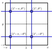
Fig. 2: A $2\times 2$ GE pivot (black circles) and corresponding rows and columns (blue lines). We only select pivots of this form during the GE procedure. The dotted lines hint at the BMC structure of the function, see (4).

After some deliberation, one concludes that if the pivots $(\lambda^{*},\theta^{*})\in[0,\pi]^{2}$ and $(\lambda^{*}-\pi,-\theta^{*})$ are picked simultaneously, then the GE step does preserve the BMC structure. Figure 2 shows an example of the $2\times 2$ pivot matrices that we are considering. To see why such $2\times 2$ pivots preserve the BMC structure, let $M$ be the associated $2\times 2$ pivot matrix given by

$$M=\begin{bmatrix}\tilde{f}(\lambda^{*}-\pi,\theta^{*})&\tilde{f}(\lambda^{*},\theta^{*})\cr\tilde{f}(\lambda^{*}-\pi,-\theta^{*})&\tilde{f}(\lambda^{*},-\theta^{*})\end{bmatrix}=\begin{bmatrix}\tilde{f}(\lambda^{*}-\pi,\theta^{*})&\tilde{f}(\lambda^{*},\theta^{*})\cr\tilde{f}(\lambda^{*},\theta^{*})&\tilde{f}(\lambda^{*}-\pi,\theta^{*})\end{bmatrix},$$ (7)

where the last equality follows from the BMC structure of $\tilde{f}$, see (3). The matrix $M$ is a $2\times 2$ centrosymmetric matrix and assuming $M$ is an invertible matrix, $M^{-1}$ is also centrosymmetric. Therefore, the corresponding GE step on a BMC function $\tilde{f}$ takes the following form:

$$\tilde{f}(\lambda,\theta)\quad\longleftarrow\quad\tilde{f}(\lambda,\theta)-\begin{bmatrix}\tilde{f}(\lambda^{*}-\pi,\theta)&\tilde{f}(\lambda^{*},\theta)\\[3.0pt] \end{bmatrix}M^{-1}\begin{bmatrix}\tilde{f}(\lambda,\theta^{*})\\[3.0pt] \tilde{f}(\lambda,-\theta^{*})\end{bmatrix}.$$ (8)

It is a simple matter now to check, using (3), that (8) preserves the BMC structure of $\tilde{f}$. The key property is that $M^{-1}$ commutes with the exchange matrix because it is centrosymmetric, i.e., $JM^{-1}=M^{-1}J$, where $J$ is the matrix formed by swapping the rows of the $2\times 2$ identity matrix.

We must go further because the GE step in (8) has two major drawbacks: (1) it is not valid unless $M$ is invertible, and (2) it suffers from severe numerical difficulties when $M$ is close to singular. To overcome these failings we replace $M^{-1}$ in (8) by the $\epsilon$-pseudoinverse of $M$, denoted by $M^{\dagger_{\epsilon}}$ [20, Sec. 5.5.2]. We deliberately leave $\epsilon\geq 0$ as an algorithmic parameter that we select later.

Definition 3.

Let $A$ be a matrix and $\epsilon\geq 0$. If $A=U\Sigma V^{*}$ is the singular value decomposition of $A$ with $\Sigma={\rm diag}(\sigma_{1},\ldots,\sigma_{n})$ and $\sigma_{k+1}\leq\epsilon<\sigma_{k}$, then

$$A^{\dagger_{\epsilon}}=V\Sigma^{\dagger_{\epsilon}}U^{*},\qquad\Sigma^{\dagger_{\epsilon}}={\rm diag}\left(\sigma_{1}^{-1},\ldots,\sigma_{k}^{-1},0,\ldots,0\right).$$

We discuss the properties of $M^{\dagger_{\epsilon}}$ in the next section, but note here that since $M$ is centrosymmetric so is $M^{\dagger_{\epsilon}}$ (see (12)). Also, the singular values of $M$ are simply

$$\sigma_{1}(M)=\max\{|a+b|,|a-b|\}\;\;\text{and}\;\;\sigma_{2}(M)=\min\{|a+b|,|a-b|\},$$ (9)

where $a=\tilde{f}(\lambda^{*}-\pi,\theta^{*})$ and $b=\tilde{f}(\lambda^{*},\theta^{*})$. Replacing $M^{-1}$ by $M^{\dagger_{\epsilon}}$ in (8) gives

$$\tilde{f}(\lambda,\theta)\quad\longleftarrow\quad\tilde{f}(\lambda,\theta)-\begin{bmatrix}\tilde{f}(\lambda^{*}-\pi,\theta)&\tilde{f}(\lambda^{*},\theta)\\[3.0pt] \end{bmatrix}M^{\dagger_{\epsilon}}\begin{bmatrix}\tilde{f}(\lambda,\theta^{*})\\[3.0pt] \tilde{f}(\lambda,-\theta^{*})\end{bmatrix}.$$ (10)

If $M$ is well-conditioned, then (10) is the same as (8) because $M^{\dagger_{\epsilon}}=M^{-1}$ when $\sigma_{2}(M)>\epsilon$. However, if $M$ is singular or near-singular, then $M^{\dagger_{\epsilon}}$ can be thought of as a surrogate for $M^{-1}$. The BMC structure of a function is preserved by (10) since $M^{\dagger_{\epsilon}}$ is still centrosymmetric, for any $\epsilon\geq 0$.

Now that (10) is valid for all nonzero $2\times 2$ pivot matrices, we want to design a strategy to pick “good” pivot matrices. This allows us to accumulate the GE updates to construct low rank approximants to the original function $\tilde{f}$. In principle, we pick $(\lambda^{*},\theta^{*})\in[0,\pi]\times[0,\pi]$ so that the resulting matrix $M$ in (7) maximizes $\sigma_{1}(M)$. This is the $2\times 2$ pivot analogue of complete pivoting. In practice, we settle for a pivot matrix that leads to a large, but not necessarily the maximum $\sigma_{1}(M)$, by searching for $(\lambda^{*},\theta^{*})$ on a coarse discrete grid of $[-\pi,\pi]\times[0,\pi]$. We have found that this pivoting strategy is very effective for constructing low rank approximants using (10).

Unfortunately, the GE procedure does not necessarily preserve the BMC-I structure of a function in the sense that the constructed rank $1$ terms in (6) do not have to be constant for $\theta=0$ and $\theta=\pm\pi$ — it is only the complete sum of all the rank $1$ terms that has this property. If $\tilde{f}$ happens to be zero along $\theta=0$ and $\theta=\pm\pi$, then each rank $1$ term will have BMC-I structure. This suggests that for a BMC-I function one can first “zero-out” the function along $\theta=0$ and $\theta=\pm\pi$ and then apply the GE procedure to the modified function. That is, we first use the rank $1$ correction:

$$\tilde{f}(\lambda,\theta)\quad\longleftarrow\quad\tilde{f}(\lambda,\theta)-\tilde{f}(\lambda^{*},\theta),$$ (11)

for some $-\pi\leq\lambda^{*}\leq\pi$. Afterwards, the GE procedure for preserving the BMC structure of a function can be used and the BMC-I structure is automatically preserved.

Figure 3 summarizes the GE algorithm that preserves the BMC structure of functions and constructs structure-preserving low rank approximations. The description given in Figure 3 is a continuous idealization of the algorithm that is used in the spherefun constructor as the continuous functions are discretized and the GE procedure is terminated after a finite number of steps. Moreover, the spherefun constructor only works on the original function $f$ on $[-\pi,\pi]\times[0,\pi]$ and mimics the GE procedure on $\tilde{f}$ by using the BMC-I symmetry. This saves a factor of $2$ in computational cost.

Algorithm: Structure-preserving GE on BMC functions Input: A BMC function $\tilde{f}$ and a coupling parameter $0\leq\alpha\leq 1$ Output: A structure-preserving low rank approximation $\tilde{f}_{k}$ to $\tilde{f}$ Set $\tilde{f}_{0}=0$ and $\tilde{e}_{0}=\tilde{f}$. for $k=1,2,3,\ldots,$     Find $(\lambda_{k},\theta_{k})$ such that $M=\begin{bmatrix}a&b\cr b&a\end{bmatrix}$, where $a=\tilde{e}_{k-1}(\lambda_{k-1}-\pi,\theta_{k-1})$ and     $b=\tilde{e}_{k-1}(\lambda_{k-1},\theta_{k-1})$ has maximal $\sigma_{1}(M)$ (see (9)).     Set $\epsilon=\alpha\sigma_{1}(M)$.     $\tilde{e}_{k}=\tilde{e}_{k-1}-\begin{bmatrix}\tilde{e}_{k-1}(\lambda_{k}-\pi,\theta)&\tilde{e}_{k-1}(\lambda_{k},\theta)\\[3.0pt] \end{bmatrix}M^{\dagger_{\epsilon}}\begin{bmatrix}\tilde{e}_{k-1}(\lambda,\theta_{k})\\[3.0pt] \tilde{e}_{k-1}(\lambda,-\theta_{k})\end{bmatrix}$.     $\tilde{f}_{k}=\tilde{f}_{k-1}-\begin{bmatrix}\tilde{e}_{k-1}(\lambda_{k}-\pi,\theta)&\tilde{e}_{k-1}(\lambda_{k},\theta)\\[3.0pt] \end{bmatrix}M^{\dagger_{\epsilon}}\begin{bmatrix}\tilde{e}_{k-1}(\lambda,\theta_{k})\\[3.0pt] \tilde{e}_{k-1}(\lambda,-\theta_{k})\end{bmatrix}$. end

Fig. 3: A continuous idealization of our structure-preserving GE procedure on BMC functions. In practice we use a discretization of this procedure and terminate it after a finite number of steps.

In practice, to make the spherefun constructor computationally efficient we use the same algorithmic ideas as in [42], with the only major difference being the pivoting strategy. Phase one of the constructor is designed to estimate the number of GE steps and pivot locations required to approximate the BMC-I function $\tilde{f}$. This costs $\mathcal{O}(K^{3})$ operations, where $K$ is the numerical rank of $\tilde{f}$. Phase two is designed to resolve the GE column and row slices and costs $\mathcal{O}(K^{2}(m+n))$ operations, where $m$ and $n$ are the number of Fourier modes needed to resolve the columns and rows, respectively. The total cost of the spherefun constructor is $\mathcal{O}(K^{3}+K^{2}(m+n))$ operations. For more implementation details on the constructor, we refer the reader to [42].

In infinite precision, one may wonder if the GE procedure in Figure 3 exactly recovers a finite rank function. This is indeed the case. That is, if $\tilde{f}$ is a function of rank $K$ in the variables $(\lambda,\theta)$, then the GE procedure terminates after constructing a rank $K$ approximation and that approximant equals $\tilde{f}$.

Theorem 4.

If $\tilde{f}$ is a rank $K$ BMC function on $[-\pi,\pi]^{2}$, then the GE procedure in Figure 3 constructs a rank $K$ approximant and $\tilde{f}$ is exactly recovered.

Proof.

Let $(\lambda^{*},\theta^{*})$ and $(\lambda^{*}-\pi,-\theta^{*})$ be the selected pivot locations in the first GE step and $M^{\dagger_{\epsilon}}$ the corresponding $2\times 2$ pivot matrix. If $M^{\dagger_{\epsilon}}$ is a rank $k$ ($k=1$ or $k=2$) matrix, then GE will form a rank $k$ update in (10). Either way, by the generalized Guttman additivity rank formula [27, Cor. 19.2], we have

$${\rm rank}(\tilde{f})={\rm rank}(M^{\dagger_{\epsilon}})+{\rm rank}\left(\tilde{f}-\begin{bmatrix}\tilde{f}(\lambda^{*}-\pi,\cdot)&\tilde{f}(\lambda^{*},\cdot)\\[3.0pt] \end{bmatrix}M^{\dagger_{\epsilon}}\begin{bmatrix}\tilde{f}(\cdot,\theta^{*})\\[3.0pt] \tilde{f}(\cdot,-\theta^{*})\end{bmatrix}\right),$$

where ${\rm rank}(\cdot)$ denotes the rank of the function or matrix. If the GE procedure constructs a rank $k$ ($k=1$ or $k=2)$ approximation in the first step, then the rank of the residual is ${\rm rank}(\tilde{f})-k$. Repeating this until the residual is of rank $0$, shows that the rank of $\tilde{f}$ and the final approximant are the same. The exact recovery result follows because the only function of rank $0$ is the zero function so the final residual is zero. ∎

A band-limited function on the sphere is one that can be expressed as a finite sum of spherical harmonics, similar to a band-limited function on the interval being expressed as a finite Fourier series. Since each spherical harmonic function is itself a rank 1 function [29, Sec. 14.30], Theorem 4 also implies that our GE procedure exactly recovers band-limited functions after a finite number of steps.

For infinite rank functions, the GE procedure in Figure 3 requires in principle an infinite number of steps. We can prove that the successive low rank approximants constructed by GE converge to $\tilde{f}$ under certain conditions on $\tilde{f}$ (see Section 3.3). Thus, the procedure can be terminated after a finite, often small, number of steps, giving an accurate low-rank approximant. In the spherefun constructor, we terminate the procedure when the residual falls below machine precision relative to an estimate of the absolute maximum of the original function.

If the parameter $\epsilon\geq 0$ for determining $M^{\dagger_{\epsilon}}$ is too large, then severely ill-conditioned pivot matrices are allowed and the algorithm suffers from a loss of accuracy. If $\epsilon$ is too small, then $M^{\dagger_{\epsilon}}$ is almost always of rank $1$ and Theorem 4 shows that the progress of GE is hindered. We choose $\epsilon$ to be $\epsilon=\alpha\sigma_{1}(M)$, where $\alpha=1/100$. In other words, we use $M^{-1}$ in the GE step if $\sigma_{1}(M)/\sigma_{2}(M)<100$ and $M^{\dagger_{\epsilon}}$ otherwise. We call $\alpha$ the coupling parameter for reasons that are explained in Section 3.2.

Figure 4 shows the importance of constructing approximants that preserve the BMC-I structure of functions on the sphere since an artificial pole singularity is introduced in each rank $1$ term when the structure is not, reducing the accuracy for derivatives. A close inspection of subplots (e) and (f) reveals pole singularities.

\begin{overpic}[width=433.62pt]{spherefun_Rank2.png} \put(0.0,85.0){(a)} \end{overpic}

\begin{overpic}[width=433.62pt]{spherefun_Rank4.png} \put(0.0,85.0){(b)} \end{overpic}

\begin{overpic}[width=433.62pt]{spherefun_Rank8.png} \put(0.0,85.0){(c)} \end{overpic}

\begin{overpic}[width=433.62pt]{spherefun_Rank16.png} \put(0.0,85.0){(d)} \end{overpic}

\begin{overpic}[width=433.62pt]{chebfun2_Rank2.png} \put(0.0,85.0){(e)} \end{overpic}

\begin{overpic}[width=433.62pt]{chebfun2_Rank4.png} \put(0.0,85.0){(f)} \end{overpic}

\begin{overpic}[width=433.62pt]{chebfun2_Rank8.png} \put(0.0,85.0){(g)} \end{overpic}

\begin{overpic}[width=433.62pt]{chebfun2_Rank16.png} \put(0.0,85.0){(h)} \end{overpic}

Fig. 4: Low rank approximants to $\tilde{f}$ in (1). Figures (a)-(d) are the respective rank 2, 4, 8, and 16 approximants to $\tilde{f}$ constructed by the structure-preserving GE procedure in Section 3.1. Figures (e)-(h) are the respective rank 2, 4, 8, and 16 approximants to $\tilde{f}$ constructed by the GE procedure that is not designed to preserve the BMC-I structure [42]. In figures (e) and (f) one can see that a pole singularity is introduced when structure is not preserved.

Our GE procedure samples $\tilde{f}$ along a sparse collection of lines, known as a skeleton [42], to construct a low rank approximation. This can be seen from the GE step in (10), which only requires 1D slices of $\tilde{f}$. Thus, $\tilde{f}$ is sampled on a grid that is not clustered near the pole of the sphere, unless it has properties that requires this. Instead, the sample points used for approximating $\tilde{f}$ are determined adaptively by the GE procedure and are composed of a criss-cross of 1D uniform grids. This means that we can take advantage of the low rank structure of functions, while still employing fast FFT-based algorithms. Figure 5 shows the skeleton selected by the GE procedure when constructing a rank $17$ approximant of the function $f(x,y,z)=\cos(xz-\sin y)$.

3.2 Another interpretation of our Gaussian elimination procedure

The GE procedure in Figure 3 that employs $2\times 2$ pivots can also be interpreted as two coupled GE procedures, with a coupling strength of $0\leq\alpha\leq 1$. This interpretation connects our method for approximating functions on the sphere to existing approximation techniques involving even-odd modal decompositions [50].

Let $\tilde{f}$ be a BMC function and $M$ be the first $2\times 2$ pivot matrix defined in (7) and written as $M=\begin{bmatrix}a&b\\ b&a\end{bmatrix}$. A straightforward derivation shows $M^{\dagger_{\epsilon}}$ can be expressed as

$$M^{\dagger_{\epsilon}}=\begin{bmatrix}\frac{1}{\sqrt{2}}&\frac{1}{\sqrt{2}}\\ \frac{1}{\sqrt{2}}&-\frac{1}{\sqrt{2}}\end{bmatrix}\begin{bmatrix}m^{\textnormal{{\tiny+}}}&\phantom{\frac{1}{\sqrt{2}}}\\ \phantom{\frac{1}{\sqrt{2}}}&m^{\textnormal{{\tiny--}}}\end{bmatrix}\begin{bmatrix}\frac{1}{\sqrt{2}}&\frac{1}{\sqrt{2}}\\ \frac{1}{\sqrt{2}}&-\frac{1}{\sqrt{2}}\end{bmatrix},$$ (12)

where the possible values of $m^{\textnormal{{\tiny+}}}$ and $m^{\textnormal{{\tiny--}}}$ are given by

$$(m^{\textnormal{{\tiny+}}},m^{\textnormal{{\tiny--}}})=\begin{cases}(1/(a+b),0),&\text{if $|a-b|<\alpha|a+b|$},\\ (0,1/(a-b)),&\text{if $|a+b|<\alpha|a-b|$},\\ (1/(a+b),1/(a-b)),&\text{otherwise}.\\ \end{cases}$$ (13)

Recall from the previous section that $\alpha=\epsilon/\sigma_{1}(M)=\epsilon/\max\{|a+b|,|a-b|\}$ and we set $\alpha=1/100$. If neither the first or second cases applies in (13), then $M^{\dagger_{\epsilon}}=M^{-1}$.

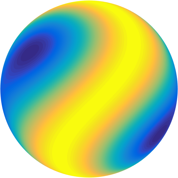
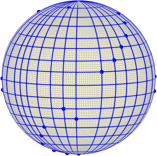
Fig. 5: Left: The function $f(x,y,z)=\cos(xz-\sin y)$ on the unit sphere. Right: The “skeleton” used to approximate $f$ by spherefun. The blue dots are the entries of the $2\times 2$ pivot matrices used by GE. The GE procedure only samples $f$ along the blue lines. The underlying tensor grid (in gray) shows the sampling grid required without low rank techniques, which cluster near the poles.

We can use (12) to re-write the GE step in (10) as

$$\tilde{f}(\lambda,\theta)\quad\longleftarrow\quad\tilde{f}(\lambda,\theta) -\frac{m^{\textnormal{{\tiny+}}}}{2}\left(\tilde{f}(\lambda^{*}-\pi,\theta)+\tilde{f}(\lambda^{*},\theta)\right)\left(\tilde{f}(\lambda,\theta^{*})+\tilde{f}(\lambda,-\theta^{*})\right)$$ (14)

$$-\frac{m^{\textnormal{{\tiny--}}}}{2}\left(\tilde{f}(\lambda^{*}-\pi,\theta)-\tilde{f}(\lambda^{*},\theta)\right)\left(\tilde{f}(\lambda,\theta^{*})-\tilde{f}(\lambda,-\theta^{*})\right).$$

Now we make a key observation. Let $f^{\textnormal{{\tiny+}}}=g+h$ and $f^{\textnormal{{\tiny--}}}=g-h$, where $g$ and $h$ are defined in (3), and note that we can decompose $\tilde{f}$ into a sum of two BMC functions:

$$\tilde{f}=\frac{1}{2}\underbrace{\begin{bmatrix}f^{\textnormal{{\tiny+}}}&f^{\textnormal{{\tiny+}}}\\ {\tt flip}(f^{\textnormal{{\tiny+}}})&{\tt flip}(f^{\textnormal{{\tiny+}}})\end{bmatrix}}_{=\tilde{f}^{\textnormal{{\tiny+}}}}+\frac{1}{2}\underbrace{\begin{bmatrix}f^{\textnormal{{\tiny--}}}&-f^{\textnormal{{\tiny--}}}\\ -{\tt flip}(f^{\textnormal{{\tiny--}}})&{\tt flip}(f^{\textnormal{{\tiny--}}})\end{bmatrix}}_{=\tilde{f}^{\textnormal{{\tiny--}}}}.$$ (15)

Using the definitions of $\tilde{f}^{\textnormal{{\tiny+}}}$ and $\tilde{f}^{\textnormal{{\tiny--}}}$ in this decomposition, the GE step in (14) can then be written as

$$\tilde{f}(\lambda,\theta)\;\longleftarrow\;\frac{1}{2}(\tilde{f}^{\textnormal{{\tiny+}}}(\lambda,\theta)-m^{\textnormal{{\tiny+}}}\tilde{f}^{\textnormal{{\tiny+}}}(\lambda^{*},\theta)\tilde{f}^{\textnormal{{\tiny+}}}(\lambda,\theta^{*}))+\frac{1}{2}(\tilde{f}^{\textnormal{{\tiny--}}}(\lambda,\theta)-m^{\textnormal{{\tiny--}}}\tilde{f}^{\textnormal{{\tiny--}}}(\lambda^{*},\theta)\tilde{f}^{\textnormal{{\tiny--}}}(\lambda,\theta^{*})),$$ (16)

which hints that the step is equivalent to two coupled GE steps on the functions $\tilde{f}^{\textnormal{{\tiny+}}}$ and $\tilde{f}^{\textnormal{{\tiny--}}}$. This connection can be made complete by noting that $a+b=\tilde{f}^{\textnormal{{\tiny+}}}(\lambda^{*},\theta^{*})$ and $a-b=\tilde{f}^{\textnormal{{\tiny--}}}(\lambda^{*},\theta^{*})$ in the definition of $m^{\textnormal{{\tiny+}}}$ and $m^{\textnormal{{\tiny--}}}$ in (13).

The coupling of the two GE steps in (16) is through the parameter $\alpha$ used to define $M^{\dagger_{\epsilon}}$. From (13) we see that when $|\tilde{f}^{\textnormal{{\tiny--}}}(\lambda^{*},\theta^{*})|<\alpha|\tilde{f}^{\textnormal{{\tiny+}}}(\lambda^{*},\theta^{*})|$, the GE step applies only to $\tilde{f}^{\textnormal{{\tiny+}}}$. Since we select the pivot matrix $M$ so that $\sigma_{1}(M)$ (see Figure 3) is maximal, this step corresponds to GE with complete pivoting on $\tilde{f}^{\textnormal{{\tiny+}}}$ and does not alter $\tilde{f}^{\textnormal{{\tiny--}}}$. Similarly, a GE step with complete pivoting is done on $\tilde{f}^{\textnormal{{\tiny--}}}$ when $|\tilde{f}^{\textnormal{{\tiny+}}}(\lambda^{*},\theta^{*})|<\alpha|\tilde{f}^{\textnormal{{\tiny--}}}(\lambda^{*},\theta^{*})|$. If neither of these conditions is met, then (16) corresponds to an interesting mix between a GE step on $\tilde{f}^{\textnormal{{\tiny+}}}$ (or $\tilde{f}^{\textnormal{{\tiny--}}}$) with complete pivoting and another GE step on $\tilde{f}^{\textnormal{{\tiny--}}}$ (or $\tilde{f}^{\textnormal{{\tiny+}}}$) with a nonstandard pivoting strategy.

If one takes $\alpha=1$, then the GE steps in (16) on $\tilde{f}^{\textnormal{{\tiny+}}}$ and $\tilde{f}^{\textnormal{{\tiny--}}}$ are fully decoupled. In this regime the algorithm in Section 3.1 is equivalent to applying GE with complete pivoting to $\tilde{f}^{\textnormal{{\tiny+}}}$ and $\tilde{f}^{\textnormal{{\tiny--}}}$ independently. There is a fundamental issue with this. The rank $1$ terms attained from applying GE to $\tilde{f}^{\textnormal{{\tiny+}}}$ and $\tilde{f}^{\textnormal{{\tiny--}}}$ can not be properly ordered when constructing a low-rank approximant of $\tilde{f}$. By selecting $\alpha<1$, the GE steps are coupled and the rank $1$ terms are (partially) ordered. This also means that a GE step can achieve a rank $2$ update, which reduces the number of pivot searches and improves the overall efficiency of the spherefun constructor.

The decomposition $\tilde{f}=\frac{1}{2}f^{\textnormal{{\tiny+}}}+\frac{1}{2}f^{\textnormal{{\tiny--}}}$ is also important for identifying symmetries that a BMC function obtained from the DFS method must possess. From (15) we see that the function $\tilde{f}^{\textnormal{{\tiny+}}}$ is an even function in $\theta$ and $\pi$-periodic in $\lambda$, while $\tilde{f}^{\textnormal{{\tiny--}}}$ is an odd function in $\theta$ and $\pi$-antiperiodic in $\lambda$. This even-periodic/odd-antiperiodic decomposition of a BMC function has been used in various guises in the DFS method as detailed in [50]. However, in these studies the representations of $\tilde{f}$ were constructed in a purely modal fashion, where the symmetries were enforced directly on the 2D Fourier coefficients of $\tilde{f}$. The representation of $\tilde{f}$ in (15) shows how to enforce these symmetries in a purely nodal fashion, i.e., on the values of the function, which appears to be a new observation. Our GE procedure produces a low rank approximation to $\tilde{f}$ that preserves these even-periodic and odd-antiperiodic symmetries.

We conclude this section by noting another important result of the decomposition of the pseudoinverse of the $2\times 2$ pivot matrices in (12). Applying this decomposition to each pivot matrix after the GE procedure in Figure 3 terminates, allows us to write the low rank function that results from the algorithm in the form of (6), with $d_{j}$ given by the eigenvalues of the pseudoinverse of the pivot matrices. Furthermore, using (16), we can split the approximation as

$$\tilde{f}(\lambda,\theta)\approx\sum_{j=1}^{K}d_{j}c_{j}(\theta)r_{j}(\lambda)=\sum_{j=1}^{K^{\textnormal{{\tiny+}}}}d^{\textnormal{{\tiny+}}}_{j}{c}^{\textnormal{{\tiny+}}}_{j}(\theta){r}^{\textnormal{{\tiny+}}}_{j}(\lambda)+\sum_{j=1}^{K^{\textnormal{{\tiny--}}}}d^{\textnormal{{\tiny--}}}_{j}{c}^{\textnormal{{\tiny--}}}_{j}(\theta){r}^{\textnormal{{\tiny--}}}_{j}(\lambda),$$ (17)

where $K^{\textnormal{{\tiny+}}}+K^{\textnormal{{\tiny--}}}=K$. Here, the functions ${c}^{\textnormal{{\tiny+}}}_{j}(\theta)$ and ${r}^{\textnormal{{\tiny+}}}_{j}(\lambda)$ for $1\leq j\leq K$ are even and $\pi$-periodic, while ${c}^{\textnormal{{\tiny--}}}_{j}(\theta)$ and ${r}^{\textnormal{{\tiny--}}}_{j}(\lambda)$ for $1\leq j\leq K$ are odd and $\pi$-antiperiodic. If $\tilde{f}$ is non-zero at the poles and (11) is employed in the first step of the GE procedure, then ${c}^{\textnormal{{\tiny+}}}_{1}(\theta)=\tilde{f}(\lambda^{*},\theta)$, ${r}^{\textnormal{{\tiny+}}}_{1}(\lambda)=1$, and $d^{\textnormal{{\tiny+}}}_{1}=1$. The two summations after the last equal sign in (17) provide low rank approximations to $\tilde{f}^{\textnormal{{\tiny+}}}$ and $\tilde{f}^{\textnormal{{\tiny--}}}$, respectively. The BMC-I structure of the approximation (17) then becomes obvious.

3.3 Analyzing the structure-preserving Gaussian elimination procedure

GE on matrices with partial pivoting is known to be theoretically unstable in the worst case because each step can increase the absolute magnitude of the matrix entries by a factor of $2$. Even though in practice this instability is extraordinarily rare, for a convergence theorem we need to control the worst-case behavior.

The so-called growth factor quantifies the worst possible increase in the absolute maximum after a rank one update. The following theorem gives a bound on the growth factor for our structure-preserving GE procedure in Figure 3.

Lemma 5.

The growth factor for the structure-preserving GE procedure in Figure 3 is $\leq\max(3,\sqrt{1+4/\alpha})$, where $\alpha$ is the coupling parameter.

Proof.

It is sufficient to examine the growth factor of the first GE step. Let $M$ be the first $2\times 2$ pivot matrix so that $M$ is the matrix of the form in (7) that maximizes $\sigma_{1}(M)$. Since $M$ maximizes $\sigma_{1}(M)$ and using (9), we have $\sigma_{1}(M)\geq\|\tilde{f}\|_{\infty}$, where $\|\tilde{f}\|_{\infty}$ denotes the absolute maximum of $\tilde{f}$ on $[-\pi,\pi]^{2}$. There are two cases to consider.

Case $1$: $\sigma_{2}(M)<\alpha\sigma_{1}(M)$. Here $M^{\dagger_{\epsilon}}$ in (10) with $\epsilon=\alpha\sigma_{1}(M)$ is of rank $1$ and the explicit formula for the spectral decomposition of $M^{\dagger_{\epsilon}}$ in (12) shows that

$$\left\|\tilde{f}-\begin{bmatrix}\tilde{f}(\lambda^{*}-\pi,\cdot)&\tilde{f}(\lambda^{*},\cdot)\\[3.0pt] \end{bmatrix}M^{\dagger_{\epsilon}}\begin{bmatrix}\tilde{f}(\cdot,\theta^{*})\\[3.0pt] \tilde{f}(\cdot,-\theta^{*})\end{bmatrix}\right\|_{\infty}\leq\|\tilde{f}\|_{\infty}+\frac{2\|\tilde{f}\|_{\infty}^{2}}{\sigma_{1}(M)}\leq 3\|\tilde{f}\|_{\infty},$$

where in the last equality we used $\sigma_{1}(M)\geq\|\tilde{f}\|_{\infty}$. Thus, the growth factor here is $\leq 3$.

Case $2$: $\sigma_{2}(M)\geq\alpha\sigma_{1}(M)$. Here $M^{\dagger_{\epsilon}}=M^{-1}$ and

$$\|M^{-1}\|_{\max}\leq\frac{\|\tilde{f}\|_{\infty}}{{\rm det}(M)}=\frac{\|\tilde{f}\|_{\infty}}{\sigma_{1}(M)\sigma_{2}(M)}\leq\frac{\|\tilde{f}\|_{\infty}}{\alpha\sigma_{1}(M)^{2}}\leq\frac{1}{\alpha\|\tilde{f}\|_{\infty}},$$

where $\|M^{-1}\|_{\max}$ denotes the maximum absolute entry of $M^{-1}$. Therefore, we have

$$\left\|\tilde{f}-\begin{bmatrix}\tilde{f}(\lambda^{*}-\pi,\cdot)&\tilde{f}(\lambda^{*},\cdot)\\[3.0pt] \end{bmatrix}M^{\dagger_{\epsilon}}\begin{bmatrix}\tilde{f}(\cdot,\theta^{*})\\[3.0pt] \tilde{f}(\cdot,-\theta^{*})\end{bmatrix}\right\|_{\infty}\leq\|\tilde{f}\|_{\infty}+\frac{4\|\tilde{f}\|_{\infty}}{\alpha}\leq\left(1+\frac{4}{\alpha}\right)\|\tilde{f}\|_{\infty}.$$

Thus, the growth factor here is $\leq\sqrt{1+4/\alpha}$ because the GE update is of rank $2$. ∎

Bounding the growth factor leads to a GE convergence result for continuous functions $\tilde{f}(\lambda,\theta)$ that satisfy the following property: for each fixed $\theta\in[-\pi,\pi]$, $\tilde{f}(\cdot,\theta)$ is an analytic function in a sufficiently large neighborhood of the complex plane containing $[-\pi,\pi]$. In approximation theory it is common to consider the neighborhood known as the stadium of radius $\beta>0$, denoted by $S_{\beta}$.

Definition 6.

Let $S_{\beta}$ with $\beta>0$ be the “stadium” of radius $\beta$ in the complex plane consisting of all numbers lying at a distance $\leq\beta$ from an interval $[a,b]$, i.e.,

$$S_{\beta}=\left\{z\in\mathbb{C}:\inf_{x\in[a,b]}|x-t|\leq\beta\right\}.$$

In the statement of the following theorem the roles of $\lambda$ and $\theta$ can be exchanged.

Theorem 7.

Let $\tilde{f}:[-\pi,\pi]^{2}\rightarrow\mathbb{C}$ be a BMC function such that $\tilde{f}(\lambda,\cdot)$ is continuous for any $\lambda\in[-\pi,\pi]$ and $\tilde{f}(\cdot,\theta)$ is analytic and uniformly bounded in a stadium $S_{\beta}$ of radius $\beta=\max(3,\sqrt{1+4/\alpha})\rho\pi$, $\rho>1$, for any $\theta\in[-\pi,\pi]$. Then, the error after $k$ GE steps decays to zero as $k\rightarrow\infty$, i.e.,

$$\|\tilde{e}_{k}\|_{\infty}\rightarrow 0,\qquad k\rightarrow\infty.$$

That is, the sequence of approximants constructed by the structure-preserving GE procedure for $\tilde{f}$ in Figure 3 converges uniformly to $\tilde{f}$.

Proof.

Let $\tilde{e}_{k}$ be the error after $k$ GE steps in Figure 3. Since $\tilde{e}_{k}$ is a BMC function for $k\geq 0$, $\tilde{e}_{k}$ can be decomposed into the sum of an even-periodic and odd-antiperiodic function, i.e., $\tilde{e}_{k}=\tilde{e}^{\textnormal{{\tiny+}}}_{k}+\tilde{e}^{\textnormal{{\tiny--}}}_{k}$ for $k\geq 0$, as discussed in Section 3.2. Additionally, from Section 3.2, we know that the structure-preserving GE procedure in Figure 3 can regarded as two coupled GE procedure on the even-periodic and odd-antiperiodic parts; see (16).

Thus, we examine the size of $\|\tilde{e}^{\textnormal{{\tiny+}}}_{k}\|_{\infty}$ and $\|\tilde{e}^{\textnormal{{\tiny--}}}_{k}\|_{\infty}$, hoping to show that $\|\tilde{e}^{\textnormal{{\tiny+}}}_{k}\|_{\infty}\rightarrow 0$ and $\|\tilde{e}^{\textnormal{{\tiny--}}}_{k}\|_{\infty}\rightarrow 0$ as $k\rightarrow\infty$. First, note that we can write $k=k^{\textnormal{{\tiny+}}}+k^{\textnormal{{\tiny--}}}+k^{0}$, where

$$k^{\textnormal{{\tiny+}}} =\text{ the number of GE steps in which only $\tilde{e}^{\textnormal{{\tiny+}}}_{k}$ is updated},$$

$$k^{\textnormal{{\tiny--}}} =\text{ the number of GE steps in which only $\tilde{e}^{\textnormal{{\tiny--}}}_{k}$ is updated},$$

$$k^{0} =\text{ the number of GE steps in which both $\tilde{e}^{\textnormal{{\tiny+}}}_{k}$ and $\tilde{e}^{\textnormal{{\tiny--}}}_{k}$ are updated}.$$

Since $\tilde{e}^{\textnormal{{\tiny+}}}_{0}$ and $\tilde{e}^{\textnormal{{\tiny--}}}_{0}$ are continuous, the growth factor of GE at each step is $\leq\max(3,\sqrt{1+4/\alpha})$, and $\tilde{e}^{+}_{0}(\cdot,\theta)$ and $\tilde{e}^{\textnormal{{\tiny--}}}_{0}(\cdot,\theta)$ are analytic and uniformly bounded in the stadium $S_{\beta}$ of radius $\beta=\max(3,\sqrt{1+4/\alpha})\rho\pi$, $\rho>1$, for any $\theta\in[-\pi,\pi]$. We know from Theorem $8.2$ in [44], which proves the convergence of GE on functions, that

$$\|\tilde{e}^{\textnormal{{\tiny+}}}_{k}\|_{\infty}\rightarrow 0,\qquad\text{ if }\quad k^{\textnormal{{\tiny+}}}+k^{0}\rightarrow\infty,$$

$$\|\tilde{e}^{\textnormal{{\tiny--}}}_{k}\|_{\infty}\rightarrow 0,\qquad\text{ if }\quad k^{\textnormal{{\tiny--}}}+k^{0}\rightarrow\infty.$$

Since either $k^{\textnormal{{\tiny+}}}+k^{0}\rightarrow\infty$ or $k^{\textnormal{{\tiny--}}}+k^{0}\rightarrow\infty$ as $k\rightarrow\infty$, either $\|\tilde{e}^{\textnormal{{\tiny+}}}_{k}\|_{\infty}\rightarrow 0$ or $\|\tilde{e}^{\textnormal{{\tiny--}}}_{k}\|_{\infty}\rightarrow 0$.

We now set out to show that both $\|\tilde{e}^{\textnormal{{\tiny+}}}_{k}\|_{\infty}\rightarrow 0$ and $\|\tilde{e}^{\textnormal{{\tiny--}}}_{k}\|_{\infty}\rightarrow 0$ as $k\rightarrow\infty$, and we proceed by contradiction. Suppose that $\|\tilde{e}^{\textnormal{{\tiny+}}}_{k}\|_{\infty}>\delta>0$ for all $k\geq 0$ and hence, the number of steps that updated the even-periodic part is finite. Let step $K$ be the last GE step that updated the even-periodic part. Now pick $K^{*}>K$ sufficiently large so that $\|\tilde{e}^{\textnormal{{\tiny--}}}_{K^{*}}\|_{\infty}<\delta$ and note that the $K^{*}+1>K$ GE step must update the even-periodic part, contradicting that $K$ was the last step to update the even-periodic part. We conclude that $\|\tilde{e}_{k}\|_{\infty}\leq\|\tilde{e}^{\textnormal{{\tiny+}}}_{k}+\tilde{e}^{\textnormal{{\tiny--}}}_{k}\|_{\infty}\leq\|\tilde{e}^{\textnormal{{\tiny+}}}_{k}\|_{\infty}+\|\tilde{e}^{\textnormal{{\tiny+}}}_{k}\|_{\infty}\rightarrow 0$ as $k\rightarrow\infty$. ∎

We expect that one can show that the GE procedure constructs a sequence of low rank approximants that converges geometrically to $\tilde{f}$, under the same assumptions of Theorem 7. Moveover, weaker analyticity assumptions may be possible because [41] could lead to a tighter bound on the growth factor of our GE procedure. In practice, even for functions that are a few times differentiable, the low rank approximants constructed by GE converge to $\tilde{f}$, but our theorem does not prove this.

4 A collection of algorithms for numerical computations with function on the sphere

Low rank approximants have a convenient representation for integrating, differentiating, evaluating, and performing many other computational tasks. We now discuss several of these operations, which are all available in spherefun. In the discussion, we assume that $f$ is a smooth function on the sphere and has been extended to a BMC function, $\tilde{f}$, using the DFS method. Then, we suppose that the GE procedure in Figure 3 has constructed a low rank approximation of $\tilde{f}$ as in (6). The functions $c_{j}(\theta)$ and $r_{j}(\theta)$ in (6) are $2\pi$-periodic and we represent them with Fourier expansions, i.e.,

$$c_{j}(\theta)=\sum_{k=-m/2}^{m/2-1}a_{k}^{j}e^{ik\theta},\qquad r_{j}(\lambda)=\sum_{k=-n/2}^{n/2-1}b_{k}^{j}e^{ik\lambda},$$ (18)

where $m$ and $n$ are even integers. We could go further and split the functions $c_{j}$ and $r_{j}$ into the functions ${c}^{\textnormal{{\tiny+}}}_{j}$, ${r}^{\textnormal{{\tiny+}}}_{j}$, ${c}^{\textnormal{{\tiny--}}}$, and ${r}^{\textnormal{{\tiny--}}}$ in (17). In this case the Fourier coefficients of these functions would satisfy certain properties related to even/odd and $\pi$-periodic/$\pi$-antiperiodic symmetries [49].

In principle, the number of Fourier modes for $c_{j}(\theta)$ and $r_{j}(\lambda)$ in (18) could depend on $j$. Here, we use the same number of modes, $m$, for each $c_{j}(\theta)$ and, $n$, for each $r_{j}(\lambda)$. This allows operations to be more efficient as the code can be vectorized.

Pointwise evaluation

The evaluation of $f(x,y,z)$ on the surface of the sphere, i.e., when $x^{2}+y^{2}+z^{2}=1$, is computationally very efficient. In fact this immediately follows from the low rank representation for $\tilde{f}$ since

$$f(x,y,z)=\tilde{f}(\lambda,\theta)\approx\sum_{j=1}^{K}d_{j}c_{j}(\theta)r_{j}(\lambda),$$

where $\lambda=\tan^{-1}(y/x)$ and $\theta=\cos^{-1}(z/(x^{2}+y^{2})^{1/2})$. Thus, $f(x,y,z)$ can be calculated by evaluating $2K$ 1D Fourier expansions (18) using Horner’s algorithm, which requires a total of $\mathcal{O}(K(n+m))$ operations [49].

The spherefun software allows users to evaluate using either Cartesian or spherical coordinates. In the former case, points that do not satisfy $x^{2}+y^{2}+z^{2}=1$, are projected to the unit sphere in the radial direction.

Computation of Fourier coefficients

The DFS method and our low rank approximant for $\tilde{f}$ means that the FFT is applicable when computing with $\tilde{f}$. Here, we assume that the Fourier coefficients for $c_{j}$ and $r_{j}$ in (18) are unknown. In full tensor-product form the bi-periodic BMC-I function can be approximated using a 2D Fourier expansion. That is,

$$\tilde{f}(\lambda,\theta)\approx\sum_{j=-m/2}^{m/2-1}\sum_{k=-n/2}^{n/2-1}X_{jk}e^{ij\theta}e^{ik\lambda}.$$ (19)

The $m\times n$ matrix $X$ of Fourier coefficients can be directly computed by sampling $\tilde{f}$ on a 2D uniform tensor-product grid and using the 2D FFT, costing $\mathcal{O}(mn\log(mn))$ operations. The low rank structure of $\tilde{f}$ allows us to compute a low rank approximation of $X$ in $\mathcal{O}(K(m\log m+n\log n))$ operations from uniform samples of $\tilde{f}$ along the adaptively selected skeleton from Section 3. The matrix $X$ is given in low rank form as $X=ADB^{T}$, where $A$ is an $m\times K$ matrix and $B$ is an $n\times K$ matrix so that the $j$th column of $A$ and $B$ is the vector of Fourier coefficients for $c_{j}$ and $r_{j}$, respectively, and $D$ is a $K\times K$ diagonal matrix containing $d_{j}$. From the low rank format of $X$ one can calculate the entries of $X$ by matrix multiplication in $\mathcal{O}(Kmn)$ operations.

The inverse operation is to sample $\tilde{f}$ on an $m\times n$ uniform grid in $[-\pi,\pi]\times[-\pi,\pi]$ given its Fourier coefficient matrix. If $X$ is given in low rank form, then this can be achieved in $\mathcal{O}(K(m\log m+n\log n))$ operations via the inverse FFT.

These efficient algorithms are regularly employed in spherefun, especially in the Poisson solver (see Section 5). The Fourier coefficients of a spherefun object are computed by the coeffs2 command and the values of the function at a uniform $\lambda$-$\theta$ grid are computed by the command sample.

Integration

The definite integral of a function $f(x,y,z)$ over the sphere can be efficiently computed in spherefun as follows:

$$\int_{S}f(x,y,z)dx\,dy\,dz=\int_{0}^{\pi}\int_{-\pi}^{\pi}\tilde{f}(\lambda,\theta)\sin\theta\,d\lambda\,d\theta\approx\sum_{j=1}^{K}d_{j}\int_{0}^{\pi}c_{j}(\theta)\sin\theta\,d\theta\int_{-\pi}^{\pi}r_{j}(\lambda)\,d\lambda$$

Hence, the approximation of the integral of $f$ over the sphere reduces to $2K$ one-dimensional integrals involving $2\pi$-periodic functions.

Due to the orthogonality of the Fourier basis, the integrals of $r_{j}(\lambda)$ are given as

$$\int_{-\pi}^{\pi}r_{j}(\lambda)\,d\lambda=2b_{0}^{j},\qquad 1\leq j\leq K,$$

where $b_{0}^{j}$ is the zeroth Fourier coefficient of $r_{j}$ in (18). The integrals of $c_{j}(\theta)$ are over half the period so the expressions are a bit more complicated. Using symmetry and orthogonality, they work out to be

$$\int_{0}^{\pi}c_{j}(\theta)\sin\theta\,d\theta=\sum_{k=-m/2}^{m/2-1}w_{k}a_{k}^{j},\qquad 1\leq j\leq K,$$ (20)

where $w_{\pm 1}=0$ and $w_{k}=(1+e^{i\pi k})/(1-k^{2})$ for $-m/2\leq k\leq m/2-1$ and $k\neq\pm 1$. Here, $a_{k}^{j}$ are the Fourier coefficients for $c_{j}$ in (18).

Therefore, we can compute the surface integral of $f(x,y,z)$ over the sphere in $\mathcal{O}(Km)$ operations. This algorithm is used in the sum2 command of spherefun. For example, the function $f(x,y,z)=1+x+y^{2}+x^{2}y+x^{4}+y^{5}+(xyz)^{2}$ has a surface integral of $216\pi/35$ and can be calculated in spherefun as follows:

f=spherefun(@(x,y,z) 1+x+y.^2+x.^2.*y+x.^4+y.^5+(x.*y.*z).^2);
sum2(f)
ans =
    19.388114662154155

The error is computed as abs(sum2(f)-216*pi/35) and is given by $3.553\times 10^{-15}$.

Differentiation

Differentiation of a function on the sphere with respect to spherical coordinates $(\lambda,\theta)$ can lead to singularities at the poles, even for smooth functions [37]. For example, consider the simple function $f(\lambda,\theta)=\cos\theta$. The $\theta$-derivative of this function is $\sin\theta$, which is continuous on the sphere but not smooth at the poles. Fortunately, one is typically interested in the derivatives that arise in applications such as in vector calculus operations involving the gradient, divergence, curl, or Laplacian. All of these operators can be expressed in terms of the components of the surface gradient with respect to the Cartesian coordinate system [16].

Let $\mathbf{e}^{x}$, $\mathbf{e}^{y}$, and $\mathbf{e}^{z}$, denote the unit vectors in the $x$, $y$, and $z$ directions, respectively, and $\nabla_{\mathcal{S}}$ denote the surface gradient on the sphere in Cartesian coordinates. From the chain rule, we can derive the Cartesian components of $\nabla_{\mathcal{S}}$ as

$$\mathbf{e}^{x}\cdot\nabla_{\mathcal{S}}:=\frac{\partial^{\rm t}}{\partial x} =-\frac{\sin\lambda}{\sin\theta}\frac{\partial}{\partial\lambda}+\cos\lambda\cos\theta\frac{\partial}{\partial\theta},$$ (21)

$$\mathbf{e}^{y}\cdot\nabla_{\mathcal{S}}:=\frac{\partial^{\rm t}}{\partial y} =\phantom{-}\frac{\cos\lambda}{\sin\theta}\frac{\partial}{\partial\lambda}+\sin\lambda\cos\theta\frac{\partial}{\partial\theta},$$ (22)

$$\mathbf{e}^{z}\cdot\nabla_{\mathcal{S}}:=\frac{\partial^{\rm t}}{\partial z} =\phantom{-\frac{\sin\lambda}{\sin\theta}\frac{\partial}{\partial\lambda}+\cos\lambda}\sin\theta\frac{\partial}{\partial\theta}.$$ (23)

Here, the superscript ‘${\rm t}$’ indicates that these operators are tangential gradient operations. The result of applying any of these operators to a smooth function on the sphere is a smooth function on the sphere [37]. For example, applying $\partial^{t}/\partial x$ to $\cos\theta$ gives $-\cos\lambda\,\sin\theta\,\cos\theta$, which in Cartesian coordinates is $-xz$ restricted to the sphere.

As with integration, our low rank approximation for $\tilde{f}$ can be exploited to compute (21)–(23) efficiently. For example, using (18) we have

$$\frac{\partial^{\rm t}\tilde{f}}{\partial x} =-\frac{\sin\lambda}{\sin\theta}\frac{\partial\tilde{f}}{\partial\lambda}+\cos\lambda\cos\theta\frac{\partial\tilde{f}}{\partial\theta}$$ (24)

$$\approx-\sum_{j=1}^{K}\left(\frac{c_{j}(\theta)}{\sin\theta}\right)\left(\sin\lambda\,\frac{\partial r_{j}(\lambda)}{\partial\lambda}\right)+\sum_{j=1}^{K}\left(\cos\theta\,\frac{\partial c_{j}(\theta)}{\partial\theta}\right)\left(\cos\lambda\,r_{j}(\lambda)\right).$$

It follows that $\partial^{\rm t}\tilde{f}/\partial x$ can be calculated by essentially 1D algorithms involving differentiating Fourier expansions as well as multiplying and dividing them by cosine and sine. In the above expression, for example, we have

$$(\sin\lambda)\frac{\partial r_{j}(\lambda)}{\partial\lambda}=\!\!\!\sum_{k=-n/2-1}^{n/2}\!\!\!\!\!\tfrac{-(k+1)b_{k+1}^{j}+(k-1)b_{k-1}^{j}}{2}e^{ik\lambda},\quad(\cos\lambda)r_{j}(\lambda)=\!\!\!\sum_{k=-n/2-1}^{n/2}\!\!\!\!\!\tfrac{b_{k+1}^{j}+b_{k-1}^{j}}{2}e^{ik\lambda},$$

where $b_{-n/2-2}^{j}=b_{-n/2-1}^{j}=0$ and $b_{n/2}^{j}=b_{n/2+1}^{j}=0$. Note that the number of coefficients in the Fourier representations of these derivatives has increased by two modes to account for multiplication by $\sin\lambda$ and $\cos\lambda$. Similarly, we also have

$$(\cos\theta)\frac{\partial c_{j}(\theta)}{\partial\theta}=\sum_{k=-m/2-1}^{m/2+1}\frac{(k+1)ia_{k+1}^{j}+(k-1)ia_{k-1}^{j}}{2}e^{ik\theta},$$

where $a_{-m/2-2}^{j}=a_{-m/2-1}^{j}=0$ and $a_{m/2}^{j}=a_{m/2+1}^{j}=0$. Lastly, for (24) we must compute $c_{j}(\theta)/\sin\theta$. This can be done as follows:

$$\frac{c_{j}(\theta)}{\sin\theta}=\sum_{k=-m/2}^{m/2-1}(M_{\sin}^{-1}\underline{a}^{j})_{k}e^{ik\lambda},\qquad M_{\sin}=\frac{i}{2}\begin{bmatrix}0&1\cr-1&0&\ddots\cr&\ddots&\ddots&1\cr&&-1&0\end{bmatrix},$$ (25)

where $\underline{a}^{j}=(a_{-m/2}^{j},\ldots,a_{m/2-1}^{j})^{T}$. Here, $M_{\sin}^{-1}$ exists because $m$ is an even integer.

Therefore, though it appears that (24) is introducing an artificial pole singularity by the division of $\sin\theta$, this is not case. Our treatment of the artificial pole singularity by operating on the coefficients directly appears to be new. The standard technique when using spherical coordinates on a latitude-longitude grid is to shift the grid in the latitude direction so that the poles are not sampled [17, 11, 51]. In (25) there is no need to explicitly avoid the pole, it is easy to implement, and is possibly more accurate numerically than shifting the grid. This algorithm costs $\mathcal{O}(K(m+n))$ operations.

We use similar ideas to compute (22) and (23), which require a similar number of operations. They are implemented in the diff command of spherefun.

4.1 Vector-valued functions on the sphere and vector calculus

Expressing vector-valued functions that are tangent to the sphere in spherical coordinates is very inconvenient since the unit vectors in this coordinate system are singular at the poles [37]. It is therefore common practice to express vector-valued functions in Cartesian coordinates, not latitude–longitude coordinates. In Cartesian coordinates the components of the vector field are smooth and can be approximated using the low rank techniques developed in Section 3.

All the standard vector-calculus operations can be expressed in terms of the tangential derivative operators in (21)–(23). For example the surface gradient, $\nabla_{\mathcal{S}}$, of a scalar-valued function $f$ on the sphere is given by the vector

$$\nabla_{\mathcal{S}}f=\begin{bmatrix}\dfrac{\partial^{\rm t}f}{\partial x},&\dfrac{\partial^{\rm t}f}{\partial y},&\dfrac{\partial^{\rm t}f}{\partial z}\end{bmatrix}^{T},$$

where the partial derivatives are defined in (21)–(23). The surface divergence and curl of a vector field $\mathbf{f}=\begin{bmatrix}f_{1},&f_{2},&f_{3}\end{bmatrix}^{T}$ that is tangent to the sphere can also be computed using (21)–(23) as

$$\nabla_{\mathcal{S}}\cdot\mathbf{f}=\dfrac{\partial^{\rm t}f_{1}}{\partial x}+\dfrac{\partial^{\rm t}f_{2}}{\partial y}+\dfrac{\partial^{\rm t}f_{3}}{\partial z},\;\nabla_{\mathcal{S}}\times\mathbf{f}=\begin{bmatrix}\dfrac{\partial^{\rm t}f_{3}}{\partial y}-\dfrac{\partial^{\rm t}f_{2}}{\partial z},&\dfrac{\partial^{\rm t}f_{1}}{\partial z}-\dfrac{\partial^{\rm t}f_{3}}{\partial x},&\dfrac{\partial^{\rm t}f_{2}}{\partial x}-\dfrac{\partial^{\rm t}f_{1}}{\partial y}\end{bmatrix}^{T}.$$

The result of the surface curl $\nabla_{\mathcal{S}}\times\mathbf{f}$ is a vector that is tangent to the sphere.

In 2D one can define the “curl of a scalar-valued function” as the cross product of the unit normal vector to the surface and the gradient of the function. For a scalar-valued function on the sphere, the curl in Cartesian coordinates is given by

$$\mathbf{n}\times\nabla_{\mathcal{S}}f=\begin{bmatrix}y\dfrac{\partial^{\rm t}f}{\partial z}-z\dfrac{\partial^{\rm t}f}{\partial y},&z\dfrac{\partial^{\rm t}f}{\partial x}-x\dfrac{\partial^{\rm t}f}{\partial z},&x\dfrac{\partial^{\rm t}f}{\partial y}-y\dfrac{\partial^{\rm t}f}{\partial x}\end{bmatrix}^{T},$$ (26)

where $x$, $y$, and $z$ are points on the unit sphere given by (2). This follows from the fact that the unit normal vector at $(x,y,z)$ on the unit sphere is just $\mathbf{n}=(x,y,z)^{T}$.

The final vector calculus operation we consider is the vorticity of a vector field, which for a two-dimensional surface is a scalar-valued function defined as $\zeta=(\nabla_{\mathcal{S}}\times\mathbf{f})\cdot\mathbf{n}$, and can be computed based on the operators described above.

Vector-valued functions are represented by spherefunv objects, which contain three spherefun objects, one for each component of the vector-valued function. Low rank techniques described in Section 3 are employed on each component separately. The operations listed above can be computed using the grad, div, curl, and vort commands; see Figure 6 for an example.

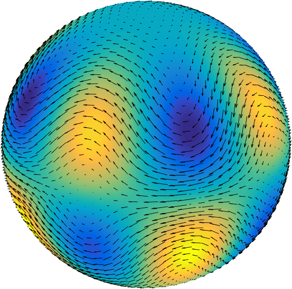
Fig. 6: Arrows indicate the tangent vector field generated from $\mathbf{u}=\nabla_{\mathcal{S}}\times\psi$, where $\psi(\lambda,\theta)=\cos\theta+(\sin\theta)^{4}\cos\theta\cos(4\lambda)$, which is the stream function for the Rossby–Haurwitz benchmark problem for the shallow water wave equations [47]. After constructing $\psi$ in spherefun, the tangent vector field was computed using u = curl(psi), and plotted using quiver(u). The superimposed false color plot represents the vorticity of $\mathbf{u}$ and is computed using vort(u).

Miscellaneous operations

The spherefun class is written as part of Chebfun, which means that spherefun objects have immediate access to all the operations available in Chebfun. For operations that do not require a strict adherence to the symmetry of the sphere, we can use Chebfun2 with spherical coordinates [42]. Important examples include two-dimensional optimization such as min2, max2, and roots as well as continuous linear algebra operators such as lu and flipud. The operations that use the Chebfun2 technology are performed seamlessly without user intervention.

5 A fast and optimal spectral method for Poisson’s equation

The DFS method leads to an efficient spectral method for solving Poisson’s equation on the sphere. The Poisson solver that we describe is simple, based on the Fourier spectral method, and has optimal complexity. Related approaches can be found in [51, 33, 12].

Given a function $f$ on the sphere satisfying $\int_{0}^{\pi}\int_{-\pi}^{\pi}f(\lambda,\theta)\sin\theta d\lambda d\theta=0$, Poisson’s equation in spherical coordinates is given by

$$(\sin\theta)^{2}\frac{\partial^{2}u}{\partial\theta^{2}}+\cos\theta\sin\theta\frac{\partial u}{\partial\theta}+\frac{\partial^{2}u}{\partial\lambda^{2}}=(\sin\theta)^{2}f,\qquad(\lambda,\theta)\in[-\pi,\pi]\times[0,\pi].$$ (27)

Due to the integral condition on $f$, (27) has infinitely many solutions, all differing by a constant. To fix this constant it is standard to solve (27) together with the constraint $\int_{0}^{\pi}\int_{-\pi}^{\pi}u(\lambda,\theta)\sin\theta d\lambda d\theta=0.$ Here, we assume that this constraint is imposed.

One can solve (27) directly on the domain $[-\pi,\pi]\times[0,\pi]$, but then the solution $u$ is not $2\pi$-periodic in the $\theta$-variable due to the coordinate transform. To recover the periodicity in $\theta$, we use the DFS method (see Section 2.2) and seek an approximation for the solution, denoted by $\tilde{u}$, to the “doubled-up” version of (27) given by

$$(\sin\theta)^{2}\tilde{u}_{\theta\theta}+\cos\theta\sin\theta\tilde{u}_{\theta}+\tilde{u}_{\lambda\lambda}=(\sin\theta)^{2}\tilde{f},\qquad(\lambda,\theta)\in[-\pi,\pi]^{2},$$ (28)

where $\tilde{f}$ is a BMC-I function that is bi-periodic, see (3). One can verify that the solution $\tilde{u}$ to (28) must also be a BMC-I function, i.e., a continuous function on the sphere. On the domain $[-\pi,\pi]\times[0,\pi]$ the solution $\tilde{u}$ in (28) must coincide with the solution $u$ to (27). Thus, we impose the same integral constraint on $\tilde{u}$:

$$\int_{0}^{\pi}\int_{-\pi}^{\pi}\tilde{u}(\lambda,\theta)\sin\theta d\lambda d\theta=0.$$ (29)

Since all the functions in (28) are bi-periodic, we discretize the equation by the Fourier spectral method [7], and $\tilde{u}$ is represented by a 2D Fourier expansion, i.e.,

$$\tilde{u}(\lambda,\theta)\approx\sum_{j=-m/2}^{m/2-1}\sum_{k=-n/2}^{n/2-1}X_{jk}e^{ij\theta}e^{ik\lambda},\qquad(\lambda,\theta)\in[-\pi,\pi]^{2},$$ (30)

where $m$ and $n$ are even integers, and seek to compute the coefficient matrix $X\in\mathbb{C}^{m\times n}$. Continuous operators, such as differentiation and multiplication, are now discretized to matrices by carefully inspecting how each operation modifies the coefficient matrix $X$ in (30) and representing the action by a matrix. For example,

$$\frac{\partial\tilde{u}}{\partial\theta}=\!\!\!\sum_{j=-m/2}^{m/2-1}\sum_{k=-n/2}^{n/2-1}\!\!\!\!jiX_{jk}e^{ij\theta}e^{ik\lambda},\quad(\cos\theta)\tilde{u}=\!\!\!\sum_{j=-m/2}^{m/2-1}\sum_{k=-n/2}^{n/2-1}\!\!\!\!\frac{X_{j+1,k}+X_{j-1,k}}{2}e^{ij\theta}e^{ik\lambda},$$

where $X_{m/2+1,k}=0$ and $X_{-m/2,k}=0$ for $-n/2-1\leq k\leq n/2$. Thus, we can represent $\partial/\partial\theta$ and multiplication by $\cos\theta$ by $D_{m}X$ and $M_{\cos}X$, respectively, where

$$D_{m}=\text{diag}\left(\left[-\tfrac{mi}{2},\cdots,\;-i,\;0,\;i,\cdots,\;\tfrac{(m-2)i}{2}\right]\right),\quad M_{\cos}=\frac{1}{2}\begin{bmatrix}0&1\cr 1&0&\ddots\cr&\ddots&\ddots&1\cr&&1&0\end{bmatrix}.$$

Similar reasoning shows that $\partial/\partial\lambda$ and multiplication by $\sin\theta$ can be discretized as $XD_{n}$ and $M_{\sin}X$, where $M_{\sin}$ is given in (25). Therefore, we can discretize (28) by the following Sylvester matrix equation:

$$\left(M_{\sin}^{2}D_{m}^{2}+M_{\cos}M_{\sin}D_{m}\right)X+XD_{n}^{2}=F,$$ (31)

where $F\in\mathbb{C}^{m\times n}$ is the matrix of 2D Fourier coefficients for $(\sin\theta)^{2}\tilde{f}$ in an expansion like (30).

We note that (31) can be solved very fast because $D_{n}$ is a diagonal matrix and hence, each column of $X$ can be found independently of the others. Writing $X=\left[X_{-n/2}\,|\,\cdots\,|\,X_{n/2-1}\right]$ and $F=\left[F_{-n/2}\,|\,\cdots\,|\,F_{n/2-1}\right]$, we can equivalently write (31) as $n$ decoupled linear systems,

$$\left(M_{\sin}^{2}D_{m}^{2}+M_{\cos}M_{\sin}D_{m}-(D_{n}^{2})_{kk}I_{m}\right)X_{k}=F_{k},\qquad-n/2\leq k\leq n/2-1,$$ (32)

where $I_{m}$ denotes the $m\times m$ identity matrix.

For $k\neq 0$, the linear systems in (32) have a pentadiagonal structure and are invertible. They can be solved by backslash, i.e., ‘\’, in MATLAB that employs a sparse LU solver. For each $k\neq 0$ this requires just $\mathcal{O}(m)$ operations, for a total of $\mathcal{O}(mn)$ operations for the linear systems in (32) with $-n/2\leq k\leq n/2-1$ and $k\neq 0$.

When $k=0$ the linear system in (32) is not invertible because we have not accounted for the integral constraint in (29), which fixes the free constant the solutions can differ by. We account for this constraint on the $k=0$ mode by noting that

$$\int_{0}^{\pi}\int_{-\pi}^{\pi}\tilde{u}(\lambda,\theta)\sin\theta d\lambda d\theta\approx 2\pi\sum_{j=-m/2}^{m/2-1}X_{j0}\frac{1+e^{i\pi j}}{1-j^{2}},$$

which can be written as $2\pi w^{T}X_{0}=0$, where the vector $w$ is given in (20). We impose $2\pi w^{T}X_{0}=0$ on $X_{0}$ by replacing the zeroth row of the linear system $(M_{\sin}^{2}D_{m}^{2}+M_{\cos}M_{\sin}D_{m})X_{0}=F_{0}$ with $2\pi w^{T}X_{0}=0$. We have selected the zeroth row because it is zero in the linear system. Thus, we solve the following linear system:

$$\begin{bmatrix}\quad w^{T}\quad\cr P\left(M_{\sin}^{2}D_{m}^{2}+M_{\cos}M_{\sin}D_{m}\right)\end{bmatrix}X_{0}=\begin{bmatrix}0\\[3.0pt] PF_{0}\end{bmatrix},$$ (33)

where $P\in\mathbb{R}^{(m-1)\times m}$ is a projection matrix that removes the zeroth row, i.e.,

$$P\left(v_{-m/2},\ldots,v_{-1},v_{0},v_{1},\ldots,v_{m/2-1}\right)^{T}=\left(v_{-m/2},\ldots,v_{-1},v_{1},\ldots,v_{m/2-1}\right)^{T}.$$

The linear system in (33) is banded with one dense row, which can be solved in $\mathcal{O}(m)$ operations using the adaptive QR algorithm [30]. For simplicity, since solving (33) is not the dominating computational cost we use the backslash command in MATLAB on sparse matrices, which requires $\mathcal{O}(m)$ operations.

The resulting Poisson solver may be regarded as having an optimal complexity of $\mathcal{O}(mn)$ because we solve for $mn$ Fourier coefficients in (30). In practice, one may need to calculate the matrix of 2D Fourier coefficients for $\tilde{f}$ that costs $\mathcal{O}(mn\log(mn))$ operations if the low rank approximation of $\tilde{f}$ is not exploited. If the low rank structure of $\tilde{f}$ is exploited, then since the whole $m\times n$ matrix coefficients $F$ is required in the Poisson solver the cost is $\mathcal{O}(mn)$ operations (see Section 4).

In Figure 7 (left) the solution to $\nabla^{2}u=\sin(50xyz)$ on the sphere is shown. Here, we used our algorithm with $m=n=150$. Before we can apply the algorithm, the matrix of 2D Fourier coefficients for $\sin(50xyz)$ is computed. Since the BMC-I function associated with $\sin(50xyz)$ has a numerical rank of $12$ this costs $\mathcal{O}(mn)$ operations. In Figure 7 (right) we verify the complexity of our Poisson solver by showing timings for $m=n$. We have denoted the number of degrees of freedom of the final solution as $mn/2$ since this is the number that is employed on the solution $u$. Without explicit parallelization, even though the solver is embarrassingly parallel, we can solve for $100$ million degrees of freedom in the solution in one minute on a standard laptop.

\begin{overpic}[width=390.25534pt,trim=120.45pt 95.35625pt 120.45pt 80.29999pt,clip]{PoissonSolution} \par\end{overpic}

\begin{overpic}[width=390.25534pt]{PoissonComplexity} \put(-5.0,15.0){\rotatebox{90.0}{{\small Computational time (sec)}}} \put(45.0,-3.0){{\small$m/2\times n$}} \put(60.0,45.0){\rotatebox{48.0}{$\mathcal{O}(mn)$}} \end{overpic}

Fig. 7: Left: Solution to $\nabla^{2}u=\sin(50xyz)$ with a zero integral constraint computed by f = spherefun(@(x,y,z) sin(50*x.*y.*z)); u = Poisson(f,0,150,150);, which employs the algorithm above with $m=n=150$. Right: Execution time of the Poisson solver as a function of the number of unknowns, $nm/2$, when $m=n$.

Conclusions

The double sphere method is synthesized with low rank approximation techniques to develop a software system for computing with functions on the sphere to essentially machine precision. We show how symmetries in the resulting functions can be preserved by an iterative variant of Gaussian elimination to efficiently construct low rank approximants. A collection of fast algorithms are developed for differentiation, integration, vector calculus, and solving Poisson’s equation. Now an investigator can compute with functions on the sphere without worrying about the underlying discretizations. The code is publicly available as part of Chebfun [14].

References

- [1] J. C. Adams and P. N. Swarztrauber, Spherepack 2.0: A Model Development Facility, Tech. Rep. NCAR/TN-436+STR, National Center for Atmospheric Research, Boulder, CO, 1997.
- [2] K. Atkinson and W. Han, Spherical Harmonics and Approximations on the Unit Sphere: An Introduction, Lecture Notes in Mathematics, Springer Berlin Heidelberg, 2012.
- [3] R. Bartnik and A. Norton, Numerical methods for the Einstein equations in null quasi-spherical coordinates, SIAM J. Sci. Comp, 22 (2000), pp. 917–950.
- [4] J. R. Baumgardner and P. O. Frederickson, Icosahedral discretization of the Two-Sphere, SIAM J. Numer. Anal., 22 (1985), pp. 1107–1115.
- [5] M. Bebendorf, Approximation of boundary element matrices, Numer. Math., 86 (2000), pp. 565–589.
- [6] J. P. Boyd, The choice of spectral functions on a sphere for boundary and eigenvalue problems: A comparison of Chebyshev, Fourier and associated Legendre expansions, Mon. Wea. Rev., 106 (1978), pp. 1184–1191.
- [7] J. P. Boyd, Chebyshev and Fourier Spectral Methods, Courier Corporation, 2001.
- [8] B. Brügmann, A pseudospectral matrix method for time-dependent tensor fields on a spherical shell, J. Comput. Phys., 235 (2013), pp. 216–240.
- [9] J. R. Bunch and B. N. Parlett, Direct methods for solving symmetric indefinite systems of linear equations, SIAM J. Numer. Anal., 8 (1971), pp. 639–655.
- [10] O. A. Carvajal, F. W. Chapman, and K. O. Geddes, Hybrid symbolic-numeric integration in multiple dimensions via tensor-product series, in Proceedings of the 2005 international symposium on Symbolic and algebraic computation, ACM, 2005, pp. 84–91.
- [11] H.-B. Cheong, Application of double Fourier series to the shallow-water equations on a sphere, J. Comput. Phys., 165 (2000), pp. 261–287.
- [12] , Double fourier series on a sphere: Applications to elliptic and vorticity equations, Journal of Computational Physics, 157 (2000), pp. 327 – 349.
- [13] J. Coiffier, Fundamentals of Numerical Weather Prediction, Cambridge University Press, 2011.
- [14] T. A. Driscoll, N. Hale, and L. N. Trefethen, eds., Chebfun Guide, Pafnuty Publications, Oxford, 2014.
- [15] G. E. Fasshauer and L. L. Schumaker, Scattered data fitting on the sphere, in Mathematical Methods for Curves and Surface, M. Daehlen, T. Lyche, and L. L. Schumaker, eds., Vanderbilt University Press, Tennessee, 1998.
- [16] N. Flyer and G. B. Wright, A radial basis function method for the shallow water equations on a sphere, in Proc. Royal Soc. A, vol. 471, The Royal Society, 2009, pp. 1–28.
- [17] B. Fornberg, A pseudospectral approach for polar and spherical geometries, SIAM J. Sci. Comp, 16 (1995), pp. 1071–1081.
- [18] B. Fornberg and D. Merrill, Comparison of finite difference and pseudospectral methods for convective flow over a sphere, Geophys. Res. Lett., 24 (1997), pp. 3245–3248.
- [19] L. V. Foster and X. Liu, Comparison of rank revealing algorithms applied to matrices with well defined numerical ranks, Manuscript, (2006).
- [20] G. Golub and C. Van Loan, Matrix Computations, Johns Hopkins University Press, 2012. Johns Hopkins Studies in the Mathematical Sciences.
- [21] K. M. Gorski, E. Hivon, A. Banday, B. D. Wandelt, F. K. Hansen, M. Reinecke, and M. Bartelmann, HEALPix: a framework for high-resolution discretization and fast analysis of data distributed on the sphere, The Astrophysical Journal, 622 (2005), p. 759.
- [22] N. Halko, P.-G. Martinsson, and J. A. Tropp, Finding structure with randomness: Probabilistic algorithms for constructing approximate matrix decompositions, SIAM review, 53 (2011), pp. 217–288.
- [23] C. Jekeli, Spherical harmonic analysis, aliasing, and filtering, Journal of Geodesy, 70 (1996), pp. 214–223.
- [24] A. T. Layton and W. F. Spotz, A semi-lagrangian double fourier method for the shallow water equations on the sphere, J. Comput. Phys., 189 (2003), pp. 180–196.
- [25] B. Leistedt, J. D. McEwen, P. Vandergheynst, and Y. Wiaux, S2LET: A code to perform fast wavelet analysis on the sphere, Astronomy & Astrophysics, 558 (2013), p. A128.
- [26] G. Martin, Transformation Geometry: An Introduction to Symmetry, Undergraduate Texts in Mathematics, Springer New York, 2012.
- [27] G. Matsaglia and G. P. H. Styan, Equalities and inequalities for ranks of matrices, Linear and multilinear Algebra, 2 (1974), pp. 269–292.
- [28] P. E. Merilees, The pseudospectral approximation applied to the shallow water equations on a sphere, Atmosphere, 11 (1973), pp. 13–20.
- [29] F. W. Olver, D. W. Lozier, R. F. Boisver, and C. W. Clark, NIST handbook of mathematical functions, Cambridge University Press, 2010.
- [30] S. Olver and A. Townsend, A fast and well-conditioned spectral method, SIAM Review, 55 (2013), pp. 462–489.
- [31] S. A. Orszag, Fourier series on spheres, Mon. Wea. Rev., 102 (1974), pp. 56–75.
- [32] R. Sadourny, Conservative finite-difference approximations of the primitive equations on quasi-uniform spherical grids, Mon. Wea. Rev., 100 (1972), pp. 136–144.
- [33] J. Shen, Efficient spectral-Galerkin methods IV. Spherical geometries, SIAM J. Sci. Comp, 20 (1999), pp. 1438–1455.
-
[34]
F. J. Simons, SLEPIAN Alpha: Release 1.0.0, Feb. 2015.
http://dx.doi.org/10.5281/zenodo.15704. - [35] W. F. Spotz, M. A. Taylor, and P. N. Swarztrauber, Fast shallow-water equation solvers in latitude-longitude coordinates, J. Comput. Phys., 145 (1998), pp. 432–444.
- [36] C. Sun, J. Li, F.-F. Jin, and F. Xie, Contrasting meridional structures of stratospheric and tropospheric planetary wave variability in the northern hemisphere, Tellus A, 66 (2014).
- [37] P. N. Swarztrauber, The approximation of vector functions and their derivatives on the sphere, SIAM J. Numer. Anal., 18 (1981), pp. 191–210.
- [38] M. Taylor, J. Tribbia, and M. Iskandarani, The spectral element method for the shallow water equations on the sphere, J. Comput. Phys., 130 (1997), pp. 92–108.
- [39] W. Tichy, Black hole evolution with the BSSN system by pseudospectral methods, Phys. Rev. D, 74 (2006), pp. 1–10.
- [40] A. Townsend, Computing with functions in two dimensions, PhD thesis, The University of Oxford, 2014.
- [41] A. Townsend, Gaussian elimination corrects pivoting mistakes, arXiv preprint arXiv:1602.06602, (2016).
- [42] A. Townsend and L. N. Trefethen, An extension of Chebfun to two dimensions, SIAM J. Sci. Comp, 35 (2013), pp. C495–C518.
- [43] , Gaussian elimination as an iterative algorithm, SIAM News, 46 (2013).
- [44] , Continuous analogues of matrix factorizations, in Proc. Royal Soc. A, vol. 471, 2015, pp. 1–21. The Royal Society.
- [45] A. Townsend, H. Wilber, and G. Wright, Computing with functions in spherical and polar geometries ii. the disk, in preparation, (2015).
-
[46]
M. Wieczorek, SHTOOLS: release 2.9.1, 2014.
http://dx.doi.org/10.5281/zenodo.12158. - [47] D. L. Williamson, J. B. Drake, J. J. Hack, R. Jakob, and P. N. Swarztrauber, A standard test set for numerical approximations to the shallow water equations in spherical geometry, J. Comput. Phys., 102 (1992), pp. 211–224.
- [48] G. B. Wright, N. Flyer, and D. A. Yuen, A hybrid radial basis function-pseudospectral method for thermal convection in a 3-D spherical shell, Geochem. Geophys. Geosyst., 11 (2010).
- [49] G. B. Wright, M. Javed, H. Montanelli, and L. N. Trefethen, Extension of Chebfun to periodic functions, SIAM J. Sci. Comp, 37 (2015), pp. C554–C573.
- [50] S. Y. K. Yee, Studies on Fourier series on spheres, Mon. Wea. Rev., 108 (1980), pp. 676–678.
- [51] , Solution of Poisson’s equation on a sphere by truncated double Fourier series, Mon. Wea. Rev., 109 (1981), pp. 501–505.