Gross-Pitaevskii vortex motion
with critically-scaled inhomogeneities
Abstract.
We study the dynamics of vortices in an inhomogeneous Gross-Pitaevskii equation . For a unique scaling regime , it is shown that vortices can interact both with the background perturbation and with each other. Results for associated parabolic and elliptic problems are discussed.
1. Introduction
We consider the behavior of vortices in an inhomogeneous Gross-Pitaevskii (IGP) equation
| (1.1) |
where is a bounded, simply connected domain in .
An important feature of solutions of (1.1) is the potential appearance of vortices, points where has a zero with nontrivial topological degree. We concentrate on the case where there are vortices of degree at positions for . We will show below that solutions take the form,
Here is interpreted in the complex sense as for with as and away from the ’s. In a sense identifying the location and degrees of vortices is sufficient to describe the solution .
The inhomogenous Gross-Pitaevskii equation (1.1) arises in several contexts, including the behavior of superfluid 4He near a boundary, Bose-Einstein Condensation (BEC) under a very weak confinement potential, and nonlinear optics. In the first case it has been observed experimentally that anomalous behavior of superfluid 4He vortex filament motion indicates that vortex tubes can become pinned to sites on the material boundary, see [46, 38, 45]. Such pinning can be incorporated heuristically by the introduction of a potential in the Gross-Pitaevskii equation, see [34] or complex Ginzburg-Landau equations, see [15]. In the second case, IGP is a useful model in a BEC in which the vortices interact both with each other and with the trap potential. In the third case, IGP is useful in modeling optical vortices. See for instance [3, 2, 34], which are related to motion of vortices with non-vanishing total charge in inhomogeneous potentials and confinement.
The dynamics of vortices in Gross-Pitaevksii equations have been the subject of much study in past few decades. The connection between the vortex motion in superfluids, where , and simplified ODE’s was made by Fetter in [11], and it was shown that vortices interact with each through a Coulomb potential. On the other hand in Bose-Einstein condensates with nontrivial trapping potentials, , it was shown by Fetter-Svidzinsky in [12] that vortices interact solely with the background potential and are carried along level sets of the Thomas-Fermi profile.
On the other hand it has been observed, both experimentally [14, 32] and numerically [29], that vortices do interact with other vortices and with the background potential. In one particularly interesting direction, experimentalists have generated dipoles by dragging non radially symmetric BEC’s through laser obstacles in [32] and by the Kibble-Zurek mechanism in [14]. These bound dipoles interact in nontrivial ways with each other and the background potentials. Reduced ODE models for the dynamics of these vortex configurations can be found in [30, 41, 42, 44] and are in good agreement with numerical simulations of the full equation (1.1) and with physical experiments, [30]. The objective of our work is to place these widely-studied models on a rigorous footing.
We are interested in the critical asymptotic regime where vortices interact with both the background potential and each other. In the following, we will take with
| (1.2) |
and show that asymptotic scalings of outside of the range (1.2) induce dynamics that are dominated by only the background potential or by only vortex-vortex interactions.
1.1. Background potential
Following Lassoued-Mironescu [26] we write
where is a minimizer of an energy (A.2) and consequently a nontrivial solution to the following elliptic PDE,
| (1.3) |
then (1.1) is equivalent to the Schrödinger equation
| (1.4) |
The local and global well-posedness of (1.4) for fixed can be established using a variation of the argument in Brezis-Gallouet [7].
Associated to (1.4) is a weighted Hamiltonian,
consequently, is the standard gauge-less Ginzburg-Landau energy density as in [4]. We set
to be the total energy of the mapping associated to background potential . We will be interested in an asymptotic range of ’s such that the resulting energy feels both the background potential and the other vortices at the same order. As will be elicited below, our regime corresponds to having the background expanded in the following way: with as .
1.2. Conservation Laws
There are a set of conservation laws for (1.4), and to write them down efficiently, we introduce some notation. For set and let us define
then solutions satisfy the following differential identities:
| (1.5) | ||||
| (1.6) |
A third conservation law holds for the Jacobian, we which we now define, tensorially. If the matrix is given by with and then and if , then following Jerrard-Smets [16] we have after a lengthy calculation
| (1.7) |
Multiplying by yields a conservation law observed in [16]
| (1.8) |
The dynamics of a vortex can be inferred by choosing suitable test functions in (1.8) which elicit the vortex positions. Since we expect the Jacobian to be roughly equal to a delta function, localized at the site of each vortex , we can choose , for smooth cutoff function in and compactly supported in . Integrating the left hand side over the support yields, formally, . On the right hand side, the first term has support in an annulus about each vortex, due to the structure of the test function, and since the energy concentrates outside of the support of the annulus, one sees that it generates an vortex-vortex interaction term. The second term on the right hand side has support inside of a ball about each vortex, and since the energy tensor is large in this region [24], it generates an vortex-potential interaction term. Therefore, for a vortex to interact with both the background potential and other vortices, it requires that for both terms to be of the same order.111The third term on the right hand side of (1.8) is negligible.
1.3. Weak Topology
In order to measure the distance of the vortices to the site of the expected location of the vortices given by the ODE (1.11), we use the flat norm . We denote the norm unless this topology is used on a subdomain, such as
We use a helpful estimate for concentrations in the flat norm, see Brezis-Coron-Lieb [6]. Define
| (1.9) |
then the following holds:
Lemma 1.1.
Suppose are points in . If
then
Proof.
For a proof see [16] for example. ∎
Consequently, the flat norm provides a good way to measure the location of singularities. Since the Jacobian, , converges to a sum of weighted delta functions, we will use topology as a convenient metric to track vortex trajectories.
Associated to a set of locations and degrees we can define a canonical harmonic map, that describes the limiting harmonic map with prescribed singularities,
where harmonic is chosen so that on . We will use when there is no ambiguity.
1.4. Energy Expansion
Given a collection of vortices with centers , the Hamiltonian can be expanded out to second order with where
which will be established in the sense of -convergence in Proposition 4.3. Here will be used throughout to represent the number of vortices, is the limiting rescaled background perturbation, and is the renormalized energy that arises in the work of Bethuel-Brezis-Hélein [4] 222The authors of [4] study the case of Dirichlet boundary conditions. See the discussion in the appendix of [40] for the derivation of with Neumann boundary conditions., given by
where . In order to express the boundary terms, we define where
If we set , then we can fully express as
| (1.10) |
1.5. Discussion
Rigorous results on vortex dynamics for Gross-Pitaevskii were established when by Colliander-Jerrard [9] and also Lin-Xin [28] which showed that vortices satisfy the Kirchoff-Onsager ODE for Euler point vortices. When there is a recent result of Jerrard-Smets [16] that showed that vortices travel along level sets of the Thomas-Fermi profile. In the parabolic setting there were rigorous results by Lin [27] and Jerrard-Soner [18] when and by Jian-Song [22] when . Mixed dynamics with and further forcing terms were discussed by Serfaty-Tice [39]. A variational proof of the parabolic dynamics for was given by Sandier-Serfaty [35].
1.6. Results
We wish to describe the dynamics of vortices in (1.4). If the vortices are located at positions with degree , then the vortices move via the ODE,
| (1.11) |
where and
| (1.12) |
Given the ODE generated by (1.11), we can define the collision time,
Then for any we can define
| (1.13) |
which is the minimum vortex-vortex or vortex-boundary distance until time . Clearly .
Our main result is the following that captures both vortex-vortex and vortex-potential interactions. An important hypothesis will be that the initial data has control of the excess energy
| (1.14) |
We will shorten the notation to when the and are readily apparent.
Theorem 1.
Let where the satisfies hypotheses of Proposition 1.2 with . Let is a configuration of vortices such that , and suppose satisfies the well-preparedness hypotheses
| (1.15) |
If is a solution to (1.1) with initial data then there exists a time such that for all ,
as , where the are defined by (1.11), and is independent of .
Remark 1.1.
An important function satisfying the conditions of Proposition 1.2 below is simply is any fixed function such that has compact support inside .
One important example that arises from the Theorem 1 are dipoles that are scattered by inhomogeneities, see Remark 1.2 below and Section 5 for some illustrative numerical simulations.
Under slightly less regularity assumptions, we have a similar result for the gradient flow
| (1.16) |
with the limit equation
| (1.17) |
Theorem 2.
Remark 1.2.
There are straightforward adaptations of Theorem 1 to other contexts, including:
- •
- •
1.7. Properties of
We collect here some information required on the behavior of , as related to the background fluctuations . The discussion of the proof will be given in Appendix A and is based off of standard elliptic theory estimates, so we simply state the results that we require for the vortex dynamics here.
We write
| (1.19) |
We will assume that in with made precise below. Using results such as [10] for the Dirichlet problem, we expect that and should be quite close. We make precise the nature in which that is true in the following Proposition, which will be proved in the Appendix.
We remark here that the elliptic analysis required for the convergence that will implement in the Appendix is somewhat non-trivial, as the overall ellipticity of the underlying nonlinear elliptic problem is going to in the limit as . Hence, estimates must be done with some care, especially to understand regularity up to the boundary of our domain.
Proposition 1.2.
Let be such that in , is compactly supported strictly on the interior of for all and in . Then, for as defined in (1.3), (1.19) satisfying Neumann boundary conditions on , we have in . In particular, we have in with for integer as required for the Schrödinger dynamics below and in , for integer as required for the gradient flow dynamics.333Note, by interpolation arguments, we can actually run the convergence argument is , where by we mean for any . We chose to here work with integer Sobolev spaces for convenience. In fact, the sharp estimate would include Schauder theory estimates directly on Hölder norms, but that would require uniform convergence in , which does not seem obvious given that the term appears to vanish in the limit preventing the proof of uniform bounds of higher regularity.
Remark 1.3.
In the appendix, we will actually decompose , in which case
this convention slightly simplifies the resulting elliptic analysis.
Remark 1.4.
Similar results hold assuming Dirichlet boundary conditions, but we work here with Neumann as they are the most physically relevant.
2. Excess Energy Control
In this section we present an excess energy identity similar to [9, 20]. The influence of the background requires some modifications, so we give a full proof. The form of the estimate will be similar to that found in [5].
Proposition 2.1.
Let and assume that there exists such that . Then there exists constants and such that if , , and
then
| (2.1) |
where vanishes as . We also have
| (2.2) | ||||
| (2.3) |
Furthermore, there exists points such that
| (2.4) |
and
| (2.5) |
where is the Kronecker delta. Here is a constant depending on , , , , , , and .
Remark 2.1.
Proof.
Although it is possible to get explicit control on the error in (2.1) by a careful analysis as in [20, 25], the weaker estimate (2.1) is sufficient to prove the vortex motion law.
1. We first decompose the excess energy into
where is appropriately chosen and .
We will control terms by variants of estimates found in [20, 25, 16]. We will choose
| (2.7) |
in the following.
2. By a simple variation of a standard calculation, see for example [20],
| (2.8) |
and so our primary concern will be with estimating the integral of (2.8) on a suitable subdomain . This last term can be rewritten as
We now fix our and in order to be able to cite some estimates from [17, 20]. The tool we wish to use is in the proof of Lemma in [20], which yields an estimate given some assumptions on the Jacobian and . Let be the constant in the assumptions of Lemma from [20], which depends only on .
We follow an argument in the proof of Theorem 6.1 of [5] for fixing these constants; however, there are several new constraints including the fact that the vortex ball radius, , cannot be too small due to the need to control terms like .
We first choose . Set such that
| (2.9) |
for all , i.e. . We further restrict where comes from the assumptions in Theorem 3 of [20], needed for the localization result (2.4).
We now choose an to allow us to use the necessary array of estimates. First, we choose so that for all ,
| (2.10) |
We then set so that for all . Indeed since then , so there exists an such that for all . We next fix such that,
| (2.11) |
for all .
If then we use and in Lemma 4 of [20]. In particular (2.10) and (2.11) imply that the assumptions in Lemma 4 hold, and we find
| (2.12) |
If then again the assumptions hold for Lemma 4 of [20], and choose and so
| (2.13) |
Taking the sum over the two errors yields sufficient control on .
Finally, we note
Combining these estimates together controls term .
3. We control using the explicit control in Lemma 12 [20],
4. We now consider terms . Recall that . We set and . Recall from (2.10) that
therefore, we can invoke Theorem and Lemma of [17]:
so
| (2.14) |
Therefore,
and so (2.1) follows.
5. We next turn to the proof of (2.2) and (2.3). We first choose vortex balls ; by (2.9),
| (2.15) |
and arguing as in Step 4,
Therefore,
| (2.16) |
and so,
| (2.17) |
Finally, , (2.17), and (2.15) allow us to use (4.27) in the proof of Proposition 4.2 in [17] which in turn implies
| (2.18) |
Since , we can combine (2.1), , and (2.18) to get bound (2.2).
To prove (2.3) we use an bound on each vortex ball in Theorem 3.2.1 of [9]. Outside the vortex balls, we use use the decomposition argument; in particular, since then from (2.16). From Remark 2.1 and the above bound, one finds
due to Remark 2.1. Combining the vortex ball bound with the bound in the excised domain yields (2.3).
5. The restriction on allows us to use Theorem 3 of [20], and estimate (2.4) follows directly. To establish (2.5) we can follow the proof of Theorem 11 in [25], along with the equipartioning result of [24], which lets us localize the stress-energy tensor up to an error of order .
∎
3. Proof of Theorem 1
The proof of the vortex motion law entails first establishing the smooth evolution of the vortex paths via the compactness theorems in Section 2. The second step will compare the vortex paths with the ODE (1.11).
3.1. Lipschitz Continuity of the Vortex Paths
Proposition 3.1.
Proof.
1. We first claim that for any , there exists an such that is a continuous function on into . Since then
since the solution map is a continuous function into .
2. We use (1.8) along with the results in Proposition 2.1. Set
| (3.2) |
where
Choosing and using (1.8) and (1.15) we generate the following bound,
and so
We can now employ a diagonalization argument. Taking subsequence , we generate a dense, countable collection of times , in which depends solely on , such that the satisfy with (3.1) as . Since the collection is dense, we can take the limit as . The Lipschitz extension of the ’s on satisfy the same conditions. ∎
3.2. Vortex Dynamics
In this subsection we complete the proof of Theorem 1. We use the Lipschitz paths generated along the subsequence from Proposition 3.1. We will examine the differences between vortex paths and the ODE, which will lead eventually to a Gronwall argument.
The proof requires two technical calculations. The first describes the gradient of in terms of the canonical harmonic map .
Lemma 3.2.
Let then and the renormalized energy satisfy
| (3.3) |
where and has support in a neighborhood of the ’s.
The second technical result proves weak compactness of the supercurrent away from the vortex cores. This will be used to bound certain cross terms in the Gronwall argument. The argument is along the lines of similar proofs in [9, 28], among other places, and we sketch most of the argument.
Lemma 3.3.
Proof.
We sketch the argument in [23] for simplicity. Since
then we can control
We now focus on the last integral.
By (2.3) in Proposition 2.1 the are uniformly bounded in for all ; furthermore, the are also in for all . The uniform bounds allows us generate a Hodge decomposition, where the and
We first claim that
| (3.5) |
Since the vector at each time then we can define the unique Hodge decomposition such that
We set to be the average of over ; and consequently from the Neumann boundary conditions on ,
where we used a Hodge decomposition of that arises from differentiating and in time. In order to control the term with , we use elliptic estimates and bound
This implies , and the three bounds combine together to yield (3.4).
∎
Proof of Theorem 1.
Define
We will estimate the difference between the vortex paths , generated by (1.4), and the positions , extracted by the ODE (1.11). We also let denote the time-varying excess energy.
Recall from (1.11) that we will estimate the differences between vortex paths and the ODE positions:
| (3.6) |
Choosing a time interval and using (1.8), (3.2), (3.3), (3.6),
| (3.7) |
We can control and using our Lipschitz bounds; in particular,
| (3.8) |
where we used Lemma 10 of [20] to control the Hessian of , with a bound dependent on . Likewise, we can use Appendix A on the regularity of to bound
| (3.9) |
We now turn to the control on . For shorthand we define components and of the supercurrents, and since then
and since , then
since . We set or , both in , then from Lemma 3.3, we have that ; note this is where we needed to consider the time-integral on .
Next we control .
We can now bound
and
Finally, we bound using (2.2):
Combining together estimates generates a differential inequality,
and choosing and dividing by implies the classical Gronwall inequality with . Therefore, for all . We can then restart the problem at time and continue the dynamics until .
So far we have only shown the theorem for a subsequence. However, our argument can be applied to subsequences of any sequence of , and as the limit is independent of the chosen subsequence, we obtain convergence for without taking subsequences. ∎
4. Second order Gamma Convergence and Gradient Flow
In this section we collect and restate some of our results on the static energy in the spirit of -convergence, compare [1] for the corresponding results for . For dynamics, we show that the approach of [35] can be adapted to treat the gradient flow as opposed to the Schrödinger dynamics studied in the previous sections.
All of our arguments work with either Neumann or Dirichlet boundary conditions, just as those in [1] and [35]. For simplicity, we assume Neumann boundary conditions throughout, and sometimes comment on changes necessary for the Dirichlet case.
4.1. Further -convergence results
We discuss -convergence properties for . From this, an analysis for the original energy
can also be deduced by the Lassoued-Mironescu result [26]
| (4.1) |
that follows from the calculation
If on or on , we can deduce (4.1) in the Dirichlet or Neumann case, respectively. However, contributes very little to the energy, and all the dynamically interesting information is encoded in , so we concentrate on in the following.
Proposition 4.1.
Let be a sequence of functions with
Then the Jacobians are compact in and for a subsequence,
where are distinct points and . Furthermore,
with .
Proof.
Comparing with the standard Ginzburg-Landau energy , we clearly have
| (4.2) |
As both the minimum and the maximum can be estimated as , we obtain that the standard Ginzburg-Landau energy is bounded as
The lower bound for the energy follows from the standard Ginzburg-Landau lower bounds and (4.2). ∎
The following bound is the heart of the second order -convergence argument.
Proposition 4.2.
Proposition 4.3.
Under the assumptions of Proposition 4.1, if we have for some the sharper upper bound
then with distinct and .
Furthermore, are then bounded in for all and satisfy the energy lower bound
where is the renormalized energy defined in (1.10).
Also, there is such that
Proof.
We clearly have with depending on and as well as on . Hence we can use Ginzburg-Landau arguments of Colliander-Jerrard [9] or Alicandro-Ponsiglione [1] to obtain the claimed structure of . The bound follows from Proposition 2.1. Let now be so small that are disjoint and do not intersect . Then we apply Proposition 4.2 to obtain
In , we let be the optimal valued map as in the definition of the renormalized energy , and let be the subsequential weak limit of . Then a.e. and hence by lower semicontinuity of the Dirichlet integral,
By (4.2), we deduce that also
Using that
we obtain the claimed lower bound.
The upper bound for the penalty term has been shown in Proposition 2.1. ∎
4.2. The gradient flow
Now we study the gradient flow analog of (1.1),
| (4.3) |
Instead of deriving an equation of motion by studying the limits of the energy density, we are going to use the method of -convergence of gradient flows. This has the advantage that we will require slightly less regularity and convergence properties for the potential term than in the Schrödinger part of this article. We will follow closely the approach of Sandier-Serfaty [35] to obtain the convergence of the gradient flow of to that of . In fact, the proof goes through with almost no essential changes, and we will therefore assume the reader is familiar with the argument and some of the notation of [35] and mostly highlight the differences.
Again, we use the approach of dividing by the profile , leading to an equation for . As we assume Neumann boundary conditions for , then Neumann boundary conditions imply Neumann boundary conditions . As before, we obtain
| (4.4) |
This is the gradient flow of with respect to the scalar product on given by the quadratic form
In fact, we have for the Gâteaux derivative
and on the other hand,
so integrating by parts we see that (4.4) is a gradient flow, more precisely .
We will show that we can relate this gradient flow to that of , where for , for , we set
and we will use the following metric on (the tangential space to ):
Theorem 3.
Assume that the profiles solving (1.3) satisfy in .
Let be a family of solutions of (4.4) with initial data . Assume that satisfy in with .
Let be a solution of the system of ODEs
| (4.5) |
where is the maximal time of existence for (4.5), i.e. the smallest time such that as as , we have .
If the initial data are very well-prepared, i.e. as , then for , so we have convergence of the gradient flow of to that of . Furthermore, so the data continue to be well-prepared. Finally, we have for and any that are disjoint open balls contained in and centered at that
| (4.6) |
Remark 4.1.
See Proposition 1.2 for conditions on the potential that imply the convergence of assumed in the theorem. Note that we require less regularity and convergence than for the Schrödinger case.
Proof of Theorem 3.
The proof is mostly an exercise in changing to in the corresponding results in [35]. The main observation, which we will use repeatedly below, is that for any sequence of we have
| (4.7) |
so in particular if , then , and a similar reverse inequality.
We note that any solution of (4.4) satisfies for
as follows from multiplying (4.4) with and integrating by parts. In particular, is weakly decreasing and
Essentially verbatim as in [35, Lemma 3.4], we can show the existence of such that actually
which implies
In addition, we also have for all with the estimate and so .
We can now apply Proposition 3.2 and Proposition 3.3 of [35] to and obtain that (for a subsequence) , where with , i.e. the are constant. Corollary 7 of [36] now applies to show
As , this also implies
| (4.8) |
The last equation is the lower bound part needed for the -convergence of gradient flows argument.
The construction also proceeds almost verbatim as in Proposition 3.5 of [35]. Let satisfy and and assume that . This implies that
We set
and note that in and . Furthermore
By (2.2) we see . From (2.3) together with we deduce in . From this point we can continue as in [35], as now both and have the same properties as the analogous quantities in [35].
Now let and let a curve satisfying and . We claim that there exists a path with and the following properties:
| (4.9) | |||
| (4.10) |
for some function that is locally bounded in .
To construct this path in function space, we use the same pushing as in [35]. Let with be pairwise disjoint balls and define to be a one-parameter family of diffeomorphisms that satisfies
With the phase corrector function defined as in (3.24) of [35], set
The claim (4.9) follows as in [35], keeping in mind our observation (4.7).
To calculate the energy change along this path, we change variables and obtain with denoting the Jacobian determinant,
We now differentiate in time and set . When the derivative does not hit , the resulting terms can be dealt with exactly as in [35] by our observation (4.7). The remaining terms are
and
We note that in , . Using the uniform convergence and the fact that the logarithmic part of the energy is concentrated in the (recall Proposition 2.1 or (3.17) of [35]), we deduce that as . To show that , we recall (2.2) and note that uniformly in . Together with the results of [35] for the terms not involving derivatives of , we deduce (4.10).
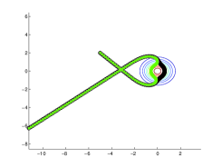
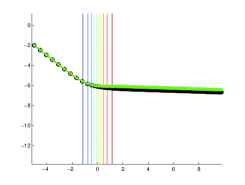
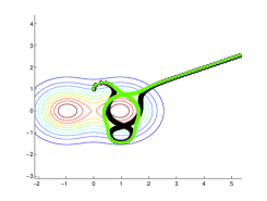
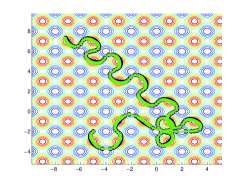
5. Numerical Simulations of the Vortex Dynamics
Armed with the dynamical equation (1.11), we can simulate the flow of vortices and observe the impact of the background potential at the scales we have studied in Theorem 1. For our simulations, we have used the renormalized energy
which is the correct expression for , see Remark 1.2. This is an approximation for the renormalized energy for for sufficiently large compared to . We will focus here on the case of the dipole (a pair of vortices of opposite charge) interacting with potentials of the form
| (5.1) | ||||
| (5.2) | ||||
| (5.3) | ||||
| (5.4) |
While these potentials are not compactly supported, we can apply Theorem 1 by truncating the potentials outside a suitably large domain without affecting the dynamics we are plotting.
Recall that in the absence of the background potential, dipole dynamics simply move in in a straight line perpendicular to that connecting the vortex centers at a speed correlated to the vortex spacing.
The equations (1.11) for each choice of background are then plugged into the ode15s ODE solver in Matlab and integrated over time scales long enough to observe the impact of the background potential on the dipole dynamics. The results are recorded graphically in Figure 1.
 |
 |
 |
 |
Appendix A Estimates on
We provide here the details required to prove Proposition 1.2. We seek to understand bounds on the function defined by
| (A.1) |
with Neumann boundary conditions, where represents the IGL background on a bounded domain .
Proof of Proposition 1.2.
1. We first claim there exists an solution for .
We use a slightly different ansatz for and :
Recall that we will assume that for with in as and is compactly supported strictly on the interior of . The last assumption in particular will be used for simplicity to allow convergence up the boundary, though this likely can be relaxed. We first claim that is the unique positive solution of the following minimization problem,
| (A.2) |
Since we are working on a bounded set , such a nontrivial exists in for sufficiently small and sufficiently bounded in using a direct method and Rellich-Kondrachov. We can improve the regularity away from the boundary. In particular if then , even though the norm blows up as . This follows from standard elliptic theory results involving nonlinear Sobolev embeddings to bootstrap regularity, see for instance [8], Section . The existence of Euler-Lagrange equations, strong solutions, and classical solutions follow.
As noted in (1.19) this is a slight shift of notation, as the defined in the main text is not quite the limit of this family of functions, rather it takes the form
The Euler-Lagrange perturbation equation is written as
| (A.3) |
and so
Then we can write this as
| (A.4) |
2. We next establish -dependent estimates on a model problem.
The required estimates follow by, for instance, carefully modifying [13][Theorem ], which draws upon ideas originally put forth by Nirenberg [33]. The proof relies upon an analysis of regularity up to the boundary by flattening locally to the half-plane and using the Green’s function there, application of difference operators to gain regularity and induction on regularity estimates for elliptic problems with Neumann boundary problems. Essentially, the argument boils down to the fact that the operator is coercive for each however. The equation also has a unique set of solutions by the same property.444Perhaps the closest argument of this type for Neumann boundary conditions can be found in [43], Chapter , Propositions and where it states that for a smooth enough domain , there exists a unique solution to the elliptic equation and for all , given , we have Since we need precise control on the constants of our estimate with respect to for a perturbation of this equation, which are not available by rescaling, we have included a proof for completeness.
To establish the bounds we need more precisely, we follow [13][Theorems and ], where the author studies Sobolev estimates on coercive elliptic equations. In our setting, these equations take the form
on smooth enough, for a bounded function of the same regularity as .
We will first consider this equation on half-balls of radius with flat boundary, say where parametrizes the boundary and parametrizes the interior. We claim we have an estimate of the form
| (A.5) |
To see this, we first claim that
| (A.6) |
with , with . For , this is exactly the coercivity estimate. Otherwise, we use an inductive argument constructed via difference operators inside the Dirichlet form for a cut-off to that vanishes on the curved part of the boundary of . Commuting with the cut-off function and integrating by parts when necessary, we observe
where then by induction we have
Similarly, we claim that
| (A.7) |
for . This follows by instead putting all the derivatives onto and using instead of norms for the term on the right hand side.
At the boundary, we can then establish (A.5), again proven using induction. To see this, we recognize that if is a multi-index and or , then the estimate follows by (A.6) and (A.7). For use the fact that
If the number of derivatives on is or , we use the above estimate. For more than that, we pull off the first two derivatives in , make the substitution, then use the inductive hypothesis.
Then, once such estimates are established on half-balls, we can create a sequence of cut-off functions , , where and can be mapped to a half-ball for and is an interior region.
Letting be a cut-off to , on the interior we have
from which the result follows via induction. On regions identified with a half-ball, we apply (A.5).
3. We can use the linear estimates (A.5) to generate a posteriori estimates on the sequence. From the energetic formulation, we have using that provides a natural set of bounds the observation
This gives
or
By a similar line of reasoning, we know that
and hence
We observe directly from (A.4) that
which gives a uniform control on in via a boot-strapping argument. Similarly, we can re-arrange (A.4) to observe
| (A.8) |
where
| (A.9) |
Hence, applying the linear estimates, we easily observe
which converges to as for sufficiently regular. Note, we have used here that has compact support in order to integrate by parts. To remove this condition otherwise would require further work controlling the error terms relating to boundary condition of and potentially restrict us to local convergence estimates.
4. To finish the a posteriori convergence, we need to get to convergence. Recall the equation
which we rewrite as
| (A.10) |
We will replace with and by the right hand side of our elliptic equation.
For higher regularity, we have the formal calculation,
where the boundary terms can be controlled by careful use of the Neumann boundary condition and the equations.
To establish the result rigorously up to the boundary, we must repeat the argument as in Step , but acting on both sides of (A.10) and then multiplying both sides by and integrating. Specifically, we can consider the coercive Dirichlet form
both in neighborhoods of the boundary, as well as in the interior to get elliptic estimates as in Step .
To see the uniqueness, let , be two solutions to (A.1) with Neumann boundary conditions for the same with for . Then set ; solves
Note that . Multiply by and integrate over , using the boundary condition:
for depending on the norms of , and so .
∎
References
- [1] R. Alicandro and M. Ponsiglione. Ginzburg-Landau functionals and renormalized energy: a revised -convergence approach. J. Funct. Anal., 266(8):4890–4907, 2014.
- [2] F. Arecchi. Space-time complexity in nonlinear optics. Physica D: Nonlinear Phenomena, 51(1–3):450 – 464, 1991.
- [3] F. Arecchi, G. Giacomelli, P. Ramazza, and S. Residori. Vortices and defect statistics in two-dimensional optical chaos. Physical review letters, 67(27):3749, 1991.
- [4] F. Bethuel, H. Brezis, and F. Hélein. Ginzburg-Landau vortices. Progress in Nonlinear Differential Equations and their Applications, 13. Birkhäuser Boston, Inc., Boston, MA, 1994.
- [5] F. Bethuel, R. L. Jerrard, and D. Smets. On the NLS dynamics for infinite energy vortex configurations on the plane. Rev. Mat. Iberoam., 24(2):671–702, 2008.
- [6] H. Brezis, J.-M. Coron, and E. H. Lieb. Harmonic maps with defects. Comm. Math. Phys., 107(4):649–705, 1986.
- [7] H. Brézis and T. Gallouet. Nonlinear Schrödinger evolution equations. Nonlinear Anal., 4(4):677–681, 1980.
- [8] H. Christianson, J. Marzuola, J. Metcalfe, and M. Taylor. Nonlinear bound states on weakly homogeneous spaces. Communications in Partial Differential Equations, 39(1):34–97, 2014.
- [9] J. E. Colliander and R. L. Jerrard. Vortex dynamics for the Ginzburg-Landau-Schrödinger equation. Internat. Math. Res. Notices, (7):333–358, 1998.
- [10] M. Dos Santos. The Ginzburg-Landau functional with a discontinuous and rapidly oscillating pinning term. Part II: the non-zero degree case. Indiana Univ. Math. J., 62(2):551–641, 2013.
- [11] A. L. Fetter. Vortices in an imperfect Bose gas. IV. Translational velocity. Phys. Rev., 151:100–104, Nov 1966.
- [12] A. L. Fetter and A. A. Svidzinsky. Vortices in a trapped dilute Bose-Einstein condensate. Journal of Physics: Condensed Matter, 13(12):R135, 2001.
- [13] G. B. Folland. Introduction to partial differential equations. Princeton University Press, 1995.
- [14] D. Freilich, D. Bianchi, A. Kaufman, T. Langin, and D. Hall. Real-time dynamics of single vortex lines and vortex dipoles in a Bose-Einstein condensate. Science, 329(5996):1182–1185, 2010.
- [15] L. Gil, K. Emilsson, and G.-L. Oppo. Dynamics of spiral waves in a spatially inhomogeneous Hopf bifurcation. Physical Review A, 45(2):R567, 1992.
- [16] R. Jerrard and D. Smets. Vortex dynamics for the two dimensional non homogeneous gross-pitaevskii equation. Annali Scuola Norm. Sup. Pisa, 14(3):729–766, 2002.
- [17] R. Jerrard and D. Spirn. Refined Jacobian estimates for Ginzburg-Landau functionals. Indiana Univ. Math. J., 56(1):135–186, 2007.
- [18] R. L. Jerrard and H. M. Soner. Dynamics of Ginzburg-Landau vortices. Arch. Rational Mech. Anal., 142(2):99–125, 1998.
- [19] R. L. Jerrard and H. M. Soner. The Jacobian and the Ginzburg-Landau energy. Calc. Var. Partial Differential Equations, 14(2):151–191, 2002.
- [20] R. L. Jerrard and D. Spirn. Refined Jacobian estimates and Gross-Pitaevsky vortex dynamics. Arch. Ration. Mech. Anal., 190(3):425–475, 2008.
- [21] R. L. Jerrard and D. Spirn. Hydrodynamic limit of the Gross-Pitaevskii equation. Communications in Partial Differential Equations, 40(2):135–190, 2015.
- [22] H.-Y. Jian and B.-H. Song. Vortex dynamics of Ginzburg-Landau equations in inhomogeneous superconductors. J. Differential Equations, 170(1):123–141, 2001.
- [23] M. Kurzke, C. Melcher, R. Moser, and D. Spirn. Dynamics for Ginzburg-Landau vortices under a mixed flow. Indiana Univ. Math. J., 58(6):2597–2621, 2009.
- [24] M. Kurzke and D. Spirn. Quantitative equipartition of the Ginzburg-Landau energy with applications. Indiana Univ. Math. J., 59(6):2077–2092, 2010.
- [25] M. Kurzke and D. Spirn. Vortex liquids and the Ginzburg–Landau equation. Forum Math. Sigma, 2:e11 (63 pages), 2014.
- [26] L. Lassoued and P. Mironescu. Ginzburg-Landau type energy with discontinuous constraint. J. Anal. Math., 77:1–26, 1999.
- [27] F. H. Lin. Some dynamical properties of Ginzburg-Landau vortices. Comm. Pure Appl. Math., 49(4):323–359, 1996.
- [28] F.-H. Lin and J. X. Xin. On the incompressible fluid limit and the vortex motion law of the nonlinear Schrödinger equation. Comm. Math. Phys., 200(2):249–274, 1999.
- [29] S. Middelkamp, P. G. Kevrekidis, D. J. Frantzeskakis, R. Carretero-González, and P. Schmelcher. Bifurcations, stability, and dynamics of multiple matter-wave vortex states. Phys. Rev. A, 82:013646, Jul 2010.
- [30] S. Middelkamp, P. J. Torres, P. G. Kevrekidis, D. J. Frantzeskakis, R. Carretero-González, P. Schmelcher, D. V. Freilich, and D. S. Hall. Guiding-center dynamics of vortex dipoles in bose-einstein condensates. Phys. Rev. A, 84:011605, Jul 2011.
- [31] E. Miot. Dynamics of vortices for the complex Ginzburg-Landau equation. Anal. PDE, 2(2):159–186, 2009.
- [32] T. Neely, E. Samson, A. Bradley, M. Davis, and B. Anderson. Observation of vortex dipoles in an oblate Bose-Einstein condensate. Physical Review Letters, 104(16):160401, 2010.
- [33] L. Nirenberg. Remarks on strongly elliptic partial differential equations. Communications on pure and applied mathematics, 8(4):648–674, 1955.
- [34] B. Y. Rubinstein and L. M. Pismen. Vortex motion in the spatially inhomogeneous conservative Ginzburg-Landau model. Phys. D, 78(1-2):1–10, 1994.
- [35] E. Sandier and S. Serfaty. Gamma-convergence of gradient flows with applications to Ginzburg-Landau. Comm. Pure Appl. Math., 57(12):1627–1672, 2004.
- [36] E. Sandier and S. Serfaty. A product-estimate for Ginzburg-Landau and corollaries. J. Funct. Anal., 211(1):219–244, 2004.
- [37] E. Sandier and S. Serfaty. Vortices in the magnetic Ginzburg-Landau model. Progress in Nonlinear Differential Equations and their Applications, 70. Birkhäuser Boston Inc., Boston, MA, 2007.
- [38] K. Schwarz. Three-dimensional vortex dynamics in superfluid He 4: Line-line and line-boundary interactions. Physical Review B, 31(9):5782, 1985.
- [39] S. Serfaty and I. Tice. Ginzburg-Landau vortex dynamics with pinning and strong applied currents. Arch. Ration. Mech. Anal., 201(2):413–464, 2011.
- [40] D. Spirn. Vortex motion law for the Schrödinger-Ginzburg-Landau equations. SIAM J. Math. Anal., 34(6):1435–1476 (electronic), 2003.
- [41] J. Stockhofe, P. G. Kevrekidis, and P. Schmelcher. Existence, Stability and Nonlinear Dynamics of Vortices and Vortex Clusters in Anisotropic Bose-Einstein Condensates, page 543. 2013.
- [42] J. Stockhofe, S. Middelkamp, P. G. Kevrekidis, and P. Schmelcher. Impact of anisotropy on vortex clusters and their dynamics. EPL (Europhysics Letters), 93(2):20008, 2011.
- [43] M. Taylor. Partial differential equations I: Basic Theory, volume 115. Springer Science & Business Media, 2013.
- [44] P. Torres, P. Kevrekidis, D. Frantzeskakis, R. Carretero-González, P. Schmelcher, and D. Hall. Dynamics of vortex dipoles in confined Bose-Einstein condensates. Physics Letters A, 375(33):3044–3050, 2011.
- [45] M. Tsubota and S. Maekawa. Pinning and depinning of two quantized vortices in superfluid He 4. Physical Review B, 47(18):12040, 1993.
- [46] E. Yarmchuk and R. Packard. Photographic studies of quantized vortex lines. Journal of Low Temperature Physics, 46(5-6):479–515, 1982.