Phase Retrieval with One or Two Diffraction Patterns by Alternating Projection with the Null Initialization

Abstract

Alternating projection (AP) of various forms, including the Parallel AP (PAP), Real-constrained AP (RAP) and the Serial AP (SAP), are proposed to solve phase retrieval with at most two coded diffraction patterns. The proofs of geometric convergence are given with sharp bounds on the rates of convergence in terms of a spectral gap condition.

To compensate for the local nature of convergence, the null initialization is proposed for initial guess and proved to produce asymptotically accurate initialization for the case of Gaussian random measurement. Numerical experiments show that the null initialization produces more accurate initial guess than the spectral initialization and that AP converges faster to the true object than other iterative schemes for non-convex optimization such as the Wirtinger Flow. In numerical experiments AP with the null initialization converges globally to the true object.

1 Introduction

With wide-ranging applications in science and technology, phase retrieval has recently attracted a flurry of activities in the mathematics community (see a recent review [55] and references therein). Chief among these applications is the coherent X-ray diffractive imaging of a single particle using a coherent, high-intensity source such as synchrotrons and free-electron lasers.

In the so-called diffract-before-destruct approach, the structural information of the sample particle is captured by an ultra-short and ultra-bright X-ray pulse and recorded by a CCD camera [18, 17, 56]. To this end, reducing the radiation exposure and damage is crucial. Due to the high frequency of the illumination field, the recorded data are the intensity of the diffracted field whose phase needs to be recovered by mathematical and algorithmic techniques. This gives rise to the problem of phase retrieval with non-crystalline structures.

The earliest algorithm of phase retrieval for a non-periodic object (such as a single molecule) is the Gerchberg-Saxton algorithm [33] and its variant, Error Reduction [31]. The basic idea is Alternating Projection (AP), going back all the way to the works of von Neuman, Kaczmarz and Cimmino in the 1930s [21, 38, 49]. And these further trace the history back to Schwarz [54] who in 1870 used AP to solve the Dirichlet problem on a region given as a union of regions each having a simple to solve Dirichlet problem.

For any vector $y$ let $|y|$ be the vector such that $|y|(j)=|y(j)|,\forall j$. In a nutshell, phase retrieval is to solve the equation of the form $b=|A^{*}x_{0}|$ where $x_{0}\in{\mathcal{X}}\subseteq\mathbb{C}^{n}$ represents the unknown object, $A^{*}\in\mathbb{C}^{N\times n}$ the diffraction/propagation process and $b^{2}\in\mathbb{R}^{N}$ the diffraction pattern(s). The subset ${\mathcal{X}}$ represents all prior constraints on the object. Also, the number of data $N$ is typically greater than the number $n$ of components in $x_{0}$.

Phase retrieval can be formulated as the following feasibility problem

(1) $$\hbox{Find}\quad\hat{y}\in A^{*}{\mathcal{X}}\cap\mathcal{Y},\quad\mathcal{Y}:=\{y\in\mathbb{C}^{N}:|y|=b\}.$$

From $\hat{y}$ the object is estimated via pseudo-inverse

(2) $$\hat{x}=(A^{*})^{\dagger}\hat{y}.$$

Let $P_{1}$ be the projection onto $A^{*}{\mathcal{X}}$ and $P_{2}$ the projection onto $\mathcal{Y}$ defined as

$$P_{2}z=b\odot{z\over|z|},\quad z\in\mathbb{C}^{N}$$

where $\odot$ denotes the Hadamard product and $z/|z|$ the componentwise division. Where $z$ vanishes, $z/|z|$ is chosen to be 1 by convention. Then AP is simply the iteration of the composite map

(3) $$P_{1}P_{2}y$$

starting with an initial guess $y^{(1)}=A^{*}x^{(1)},x^{(1)}\in{\mathcal{X}}$.

The main structural difference between AP in the classical setting [21, 38, 49] and the current setting is the non-convexity of the set $\mathcal{Y}$, rendering the latter much more difficult to analyze. Moreover, AP for phase retrieval is well known to have stagnation problems in practice, resulting in poor reconstruction [31, 32, 44].

In our view, numerical stagnation has more to do with the measurement scheme than non-convexity: the existence of multiple solutions when only one (uncoded) diffraction pattern is measured even if additional positivity constraint is imposed on the object. However, if the diffraction pattern is measured with a random mask (a coded diffraction pattern), then the uniqueness of solution under the real-valuedness constraint is restored with probability one [28]. In addition, if two independently coded diffraction patterns are measured, then the uniqueness of solution, up to a global phase factor, holds almost surely without any additional prior constraint [28] (see Proposition 1).

The main goal of the present work is to show by analysis and numerics that under the uniqueness framework for phase retrieval with coded diffraction patterns of [28], AP has a significantly sized basin of attraction at $x_{0}$ and that this basin of attraction can be reached by an effective initialization scheme, called the null initialization. In practice, numerical stagnation disappears under the uniqueness measurement schemes of [28].

Specifically, our goal is two-fold: i) prove the local convergence of various versions of AP under the uniqueness framework of [28] (Theorems 5.6, 6.3 and 7.3) and ii) propose a novel method of initialization, the null initialization, that compensates for the local nature of convergence and results in global convergence in practice. In addition, we prove that for Gaussian random measurements the null initialization alone produces an initialization of arbitrary accuracy as the sample size increases (Theorem 2.1). In practice AP with the null initialization converges globally to the true object.

1.1 Set-up

Let us recall the measurement schemes of [28].

Let $x_{0}({\mathbf{n}})$ be a discrete object function with ${\mathbf{n}}=(n_{1},n_{2},\cdots,n_{d})\in\mathbb{Z}^{d}$. Consider the object space consisting of all functions supported in

$${\mathcal{M}}=\{0\leq m_{1}\leq M_{1},0\leq m_{2}\leq M_{2},\cdots,0\leq m_{d}\leq M_{d}\}.$$

We assume $d\geq 2$.

Only the intensities of the Fourier transform, called the diffraction pattern, are measured

$$\sum_{{\mathbf{n}}=-\mathbf{M}}^{\mathbf{M}}\sum_{\mathbf{m}\in{\mathcal{M}}}x_{0}(\mathbf{m}+{\mathbf{n}})\overline{x_{0}(\mathbf{m})}e^{-i2\pi{\mathbf{n}}\cdot\mathbf{w}},\quad\mathbf{w}=(w_{1},\cdots,w_{d})\in[0,1]^{d},\quad\mathbf{M}=(M_{1},\cdots,M_{d})$$

which is the Fourier transform of the autocorrelation

$$R({\mathbf{n}})=\sum_{\mathbf{m}\in{\mathcal{M}}}x_{0}(\mathbf{m}+{\mathbf{n}})\overline{x_{0}(\mathbf{m})}.$$

Here and below the over-line means complex conjugacy.

Note that $R$ is defined on the enlarged grid

$$\widetilde{\mathcal{M}}=\{(m_{1},\cdots,m_{d})\in\mathbb{Z}^{d}:-M_{1}\leq m_{1}\leq M_{1},\cdots,-M_{d}\leq m_{d}\leq M_{d}\}$$

whose cardinality is roughly $2^{d}$ times that of ${\mathcal{M}}$. Hence by sampling the diffraction pattern on the grid

$${\mathcal{L}}=\Big{\{}(w_{1},\cdots,w_{d})\ |\ w_{j}=0,\frac{1}{2M_{j}+1},\frac{2}{2M_{j}+1},\cdots,\frac{2M_{j}}{2M_{j}+1}\Big{\}}$$

we can recover the autocorrelation function by the inverse Fourier transform. This is the standard oversampling with which the diffraction pattern and the autocorrelation function become equivalent via the Fourier transform [45, 46].

A coded diffraction pattern is measured with a mask whose effect is multiplicative and results in a masked object of the form $\tilde{x}_{0}({\mathbf{n}})=x_{0}({\mathbf{n}})\mu({\mathbf{n}})$ where $\{\mu({\mathbf{n}})\}$ is an array of random variables representing the mask. In other words, a coded diffraction pattern is just the plain diffraction pattern of a masked object.

We will focus on the effect of random phases $\phi({\mathbf{n}})$ in the mask function $\mu({\mathbf{n}})=|\mu|({\mathbf{n}})e^{i\phi({\mathbf{n}})}$ where $\phi({\mathbf{n}})$ are independent, continuous real-valued random variables and $|\mu|({\mathbf{n}})\neq 0,\forall{\mathbf{n}}\in{\mathcal{M}}$ (i.e. the mask is transparent).

For simplicity we assume $|\mu|({\mathbf{n}})=1,\forall{\mathbf{n}}$ which gives rise to a phase mask and an isometric propagation matrix

(4) $$\hbox{\rm(1-mask )}\quad A^{*}=c\Phi\,\,\mathop{\operator@font diag}\nolimits\{\mu\},$$

i.e. $AA^{*}=I$ (with a proper choice of the normalizing constant $c$), where $\Phi$ is the oversampled $d$-dimensional discrete Fourier transform (DFT). Specifically $\Phi\in\mathbb{C}^{|\tilde{\mathcal{M}}|\times|{\mathcal{M}}|}$ is the sub-column matrix of the standard DFT on the extended grid $\tilde{\mathcal{M}}$ where $|{\mathcal{M}}|$ is the cardinality of ${\mathcal{M}}$.

If the non-vanishing mask $\mu$ does not have a uniform transparency, i.e. $|\mu|({\mathbf{n}})\neq 1,\forall{\mathbf{n}},$ then we can define a new object vector $|\mu|\odot x_{0}$ and a new isometric propagation matrix

$$A^{*}=c\Phi\,\,\mathop{\operator@font diag}\nolimits\left\{{\mu\over|\mu|}\right\}$$

with which to recover the new object first.

When two phase masks $\mu_{1},\mu_{2}$ are deployed, the propagation matrix $A^{*}$ is the stacked coded DFTs, i.e.

(5) $$\hbox{(2-mask case)}\quad A^{*}=c\left[\begin{matrix}\Phi\,\,\mathop{\operator@font diag}\nolimits\{\mu_{1}\}\\ \Phi\,\,\mathop{\operator@font diag}\nolimits\{\mu_{2}\}\end{matrix}\right].$$

With proper normalization, $A^{*}$ is isometric.

We convert the $d$-dimensional ($d\geq 2$) grid into an ordered set of index. Let $n=|{\mathcal{M}}|$ and $N$ the total number of measured data. In other words, $A\in\mathbb{C}^{N\times n}$.

Let ${\mathcal{X}}$ be a nonempty closed convex set in $\mathbb{C}^{n}$ and let

(6) $$[x]_{\mathcal{X}}=\hbox{\rm arg}\min_{x^{\prime}\in{\mathcal{X}}}\|x^{\prime}-x\|$$

denote the projection onto ${\mathcal{X}}$.
Phase retrieval is to find a solution $x$ to the equation

(7) $$b=|A^{*}x|,\quad x\in{\mathcal{X}}.$$

We focus on the following two cases.

1) One-pattern case: $A^{*}$ is given by (4), ${\mathcal{X}}=\mathbb{R}^{n}$ or $\mathbb{R}^{n}_{\tiny+}$.

2) Two-pattern case: $A^{*}$ is given by (5), ${\mathcal{X}}=\mathbb{C}^{n}$ (i.e. $[x]_{\mathcal{X}}=x$).

For the two-pattern case, AP for the formulation (1) shall be called the Parallel AP (PAP) as the rows of $A^{*}$ and the diffraction data are treated equally and simultaneously, in contrast to the Serial AP (SAP) which splits the diffraction data into two blocks according to the masks and treated alternately.

The main property of the true object is the rank-$k$ property: $x_{0}$ is rank-$k$ if the convex hull of $\mathop{\operator@font supp}\nolimits\{x_{0}\}$ in $\mathbb{C}^{n}$ is $k$-dimensional.

Now we recall the uniqueness theorem of phase retrieval with coded diffraction patterns.

Proposition 1.

[28] (Uniqueness of Fourier phase retrieval) Let $x_{0}$ be a rank$-k,\leavevmode\nobreak\ k\geq 2$, object and $x$ a solution of the phase retrieval problem (7) for either the one-pattern or two-pattern case. Then $x=e^{i\theta}x_{0}$ for some constant $\theta\in\mathbb{R}$ with probability one.

Remark 1.1.

The main improvement over the classical uniqueness theorem [36] is that while the classical result works with generic (thus random) objects Proposition 1 deals with a given deterministic object. By definition, deterministic objects belong to the measure zero set excluded in the classical setting of [36]. It is crucial to endow the probability measure on the ensemble of random masks, which we can manipulate, instead of the space of unknown objects, which we can not control.

The proof of Proposition 1 is given in [28] where more general uniqueness theorems can be found, including the $1{1\over 2}$-mask case. Phase retrieval solution is unique only up to a constant of modulus one no matter how many coded diffraction patterns are measured. Thus a reasonable error metric for an estimate $\hat{x}$ of the true solution $x_{0}$ is given by

(8) $$\min_{\theta\in\mathbb{R}}\|e^{i\theta}\hat{x}-x_{0}\|.$$

Our framework and methods can be extended to more general, non-isometric measurement matrix $A^{*}$ as follows. Let $A^{*}=QR$ be the QR-decomposition of $A^{*}$ where $Q$ is isometric and $R$ is upper-triangular. We have

(9) $$Q^{*}=A^{*}(AA^{*})^{-1/2}$$

if $A$ (and hence $R$) is full-rank. Now we can define a new object vector $Rx$ and a new isometric measurement matrix $Q$ with which to recover $Rx$ first.

1.2 Other literature

Much of recent mathematical literature on phase retrieval focuses on generic frames and random measurements, see e.g. [1, 2, 3, 4, 5, 11, 15, 22, 24, 27, 35, 43, 48, 52, 55, 58, 60, 55]. Among the mathematical works on Fourier phase retrieval e.g. [7, 12, 13, 14, 19, 26, 28, 29, 30, 36, 37, 39, 40, 44, 47, 51, 16, 53, 59], only a few focus on analysis and development of efficient algorithms.

There is also vast literature on AP. We only mention the most relevant literature and refer the reader to the reviews [6, 25] for a more complete list of references. Von Neumann’s convergence theorem [49] for AP with two closed subspaces is extended to the setting of closed convex sets in [20, 10] and, starting with [33], the application of AP to the non-convex setting of phase retrieval has been extensively studied [31, 32, 7, 8, 44].

In [42] in particular, local convergence theorems were developed for AP for non-convex problems. However, the technical challenge in applying the theory in [42] to phase retrieval lies precisely in verifying the main assumption of linear regular intersection therein.

In contrast, in the present work, what guarantees the geometric convergence and gives an often sharp bound on the convergence rate is the spectral gap condition which can be readily verified under the uniqueness framework of [28] (see Propositions 5.4 and 6.1 below).

As pointed out above, there are more than one way of formulating phase retrieval, especially with two (or more) diffraction patterns, as a feasibility problem. While PAP is analogous to Cimmino’s approach to AP [21], SAP is closer in spirit to Kaczmarz’s [38]. Surprisingly, SAP performs significantly better than PAP in our simulations (Section 8). In Sections 5 and 7 we prove that both schemes are locally convergent to the true solution with bounds on rates of convergence. measurement local convergence for PAP was proved in [48].

Despite the theoretical appeal of a convex minimization approach to phase retrieval [12, 15, 14, 16], the tremendous increase in dimension results in impractically slow computation. Recently, new non-convex approaches become popular again because of their computational efficiency among other benefits [13, 47, 48].

One purpose of the present work is to compare these newer approaches with AP, arguably the simplest of all non-convex approaches. An important difference of the measurement schemes in these papers from ours is that their coded diffraction patterns are not oversampled. In this connection, we emphasize that reducing the number of coded diffraction patterns is crucial for the diffract-before-destruct approach and it is better to oversample than to increase the number of coded diffraction patterns. Another difference is that these newer iterative schemes such as the Wirtinger Flow (WF) [13] are not of the projective type. In Section 8, we provide a detailed numerical comparison between AP of various forms and WF.

Recently we proved local convergence of the Douglas-Rachford (DR) algorithm for coded-aperture phase retrieval [19]. The present work extends the method of [19] to AP. In addition to convergence analysis of AP, we also characterize the limit points and the fixed points of AP in the present work.

More important, to compensate for the local nature of convergence we develop a novel procedure, the null initialization, for finding a sufficiently close initial guess. We prove that the null initialization with the Gaussian random measurement matrix asymptotically approaches the true object (Section 2). The analogous result for coded diffraction patterns remains open. The null initialization is significantly different from the spectral initialization proposed in [48, 13, 11]. In Section 2.4 we give a theoretical comparison and in Section 8 a numerical comparison between these initialization methods. We will see that the initialization with the null initialization is more accurate than with the spectral initialization and SAP with the null initialization converges faster than the Fourier-domain Douglas-Rachford algorithm proposed in [19].

During the review process, the two references [51, 37] were brought to our attention by the referees.

Theorem 3.10 of [37] asserts global convergence to some critical point of a proximal-regularized alternating minimization formulation of (1) provided that the iterates are bounded (among other assumptions). However, neither (global or local) convergence to the true solution nor the geometric sense of convergence is established in [37]. In contrast, we prove that the AP iterates are always bounded, their accumulation points must be fixed points (Proposition 4.1) and the true solution is a stable fixed point. Moreover, any fixed point that shares the same 2-norm with the true object is the true object itself (Proposition 4.2).

On the other hand, Corollary 12 of [51] asserts the existence of a local basin of attraction of the feasible set (1) which includes AP in the one-pattern case and PAP in the two-pattern case (but not SAP). From this and the uniqueness theorem (Proposition 1) convergence to the true solution, up to a global phase factor, follows (i.e. a singleton with an arbitrary global phase factor). However, Corollary 12 of [51] asserts a sublinear power-law convergence with an unspecified power. In contrast, we prove a linear convergence and give a spectral gap bound on the convergence rate for AP, including SAP which is emphatically not covered by [51] and arguably the best performer among the tested algorithms.

The paper proceeds as follows. In Section 2, we discuss the null initialization and prove global convergence to the true object of the null initialization for the complex Gaussian random measurement. In Section 3, we formulate AP of various forms and in Section 4 we discuss the limit points and the fixed points of AP. We prove local convergence to the true solution for the Parallel AP in Section 5 and for the real-constraint AP in Section 6. In Section 7 we prove local convergence for the Serial AP. In Section 8, we present numerical experiments and compare our approach with the Wirtinger Flow and its truncated version [13, 11].

2 The null initialization

For a nonconvex minimization problem such as phase retrieval, the accuracy of the initialization as the estimate of the object has a great impact on the performance of any iterative schemes.

The following observation motivates our approach to effective initialization. Let $I$ be a subset of $\{1,\cdots,N\}$ and $I_{c}$ its complement such that $b(i)\leq b(j)$ for all $i\in I,j\in I_{c}$. In other words, $\{b(i):i\in I\}$ are the “weaker” signals and $\{b(j):j\in I_{c}\}$ the “stronger” signals. Let $|I|$ be the cardinality of the set $I$. Then $\{a_{i}\}_{i\in I}$ is a set of sensing vectors nearly orthogonal to $x_{0}$ if $|I|/N$ is sufficiently small (see Remark 2.2). This suggests the following constrained least squares solution

$$x_{\rm null}:=\hbox{\rm arg}\min\left\{\sum_{i\in I}\|a_{i}^{*}x\|^{2}:x\in{\mathcal{X}},{\|x\|=\|x_{0}\|}\right\}$$

may be a reasonable initialization. Note that $x_{\rm null}$ is not uniquely defined as $\alpha x_{\rm null}$, with $|\alpha|=1,$ is also a null vector. Hence we should consider the global phase adjustment for a given null vector $x_{\rm null}$

$$\min_{\alpha\in\mathbb{C},\;|\alpha|=1}\|\alpha x_{\rm null}-x_{0}\|^{2}=2\|x_{0}\|^{2}-2\max_{|\alpha|=1}\Re(x_{0}^{*}\alpha x_{\rm null}).$$

In what follows, we assume $x_{\rm null}$ to be optimally adjusted so that

(10) $$\|x_{\rm null}-x_{0}\|^{2}=2\|x_{0}\|^{2}-2|x_{0}^{*}x_{\rm null}|$$

We pause to emphasize that the constraint $\|x_{\rm null}\|=\|x_{0}\|$ is introduced in order to simplify the error bound below (Theorem 2.1) and is completely irrelevant to initialization since the AP map ${\mathcal{F}}$ (see (36) below for definition) is scaling-invariant in the sense that ${\mathcal{F}}(cx)={\mathcal{F}}(x)$, for any $c>0$. Also, in many imaging problems, the norm of the true object, like the constant phase factor, is either recoverable by other prior information or irrelevant to the quality of reconstruction.

Denote the sub-column matrices consisting of $\{a_{i}\}_{i\in I}$ and $\{a_{j}\}_{j\in I_{c}}$ by $A_{I}$ and $A_{I_{c}}$, respectively, and, by reordering the row index, write $A=[A_{I},A_{I_{c}}]\in\mathbb{C}^{n\times N}.$

Define the dual vector

(11) $$x_{\rm dual}:=\hbox{\rm arg}\max\left\{\|A_{I_{c}}^{*}x\|^{2}:x\in{\mathcal{X}},{\|x\|=\|x_{0}\|}\right\}$$

whose phase factor is optimally adjusted as $x_{\rm null}$.

2.1 Isometric $A^{*}$

For isometric $A^{*}$,

(12) $$x_{\rm null}:=\hbox{\rm arg}\min\left\{\sum_{i\in I}\|a_{i}^{*}x\|^{2}:x\in{\mathcal{X}},{\|x\|=\|b\|}\right\}.$$

We have

$$\|A_{I}^{*}x\|^{2}+\|A_{I_{c}}^{*}x\|^{2}=\|x\|^{2}$$

and hence

(13) $$x_{\rm null}=x_{\rm dual},$$

i.e. the null vector is self-dual in the case of isometric $A^{*}$. Eq. (13) can be used to construct the null vector from $A_{I_{c}}A^{*}_{I_{c}}$ by the power method.

Let $\mathbf{1}_{c}$ be the characteristic function of the complementary index $I_{c}$ with $|I_{c}|=\gamma N$. The default choice for $\gamma$ is the median value $\gamma=0.5$.

1

2Random initialization: $x_{1}=x_{\rm rand}$

3 Loop:

4 for $k=1:k_{\textup{max}}-1$ do

5       $x^{\prime}_{k}\leftarrow A(\mathbf{1}_{c}\odot A^{*}x_{k})$;

6       $x_{k+1}\leftarrow[x_{k}^{{}^{\prime}}]_{\mathcal{X}}/\|[x_{k}^{{}^{\prime}}]_{\mathcal{X}}\|$

7 end for

Output: $\hat{x}_{\textup{dual}}=x_{k_{\textup{max}}}$.

Algorithm 1 The null initialization

For isometric $A^{*}$, it is natural to define

(14) $$x_{\rm null}=\alpha\|b\|\cdot\hat{x}_{\rm dual},\quad\alpha={\hat{x}_{\rm dual}^{*}x_{0}\over|\hat{x}_{\rm dual}^{*}x_{0}|}$$

where $\hat{x}_{\rm dual}$ is the output of Algorithm 1. As shown in Section 8 (Fig. 8), the null vector is remarkably stable with respect to noise in $b$.

2.2 Non-isometric $A^{*}$

When $A^{*}$ is non-isometric such as the standard Gaussian random matrix (see below), the power method is still applicable with the following modification.

For a full rank $A$, let $A^{*}=QR$ be the QR-decomposition of $A^{*}$ where $Q$ is isometric and $R$ is a full-rank, upper-triangular square matrix. Let $z=Rx$, $z_{0}=Rx_{0}$ and $z_{\rm null}=Rx_{\rm null}$. Clearly, $z_{\rm null}$ is the null vector for the isometric phase retrieval problem $b=|Qz|$ in the sense of (12).

Let $I$ and $I_{c}$ be the index sets as above. Let

(15) $$\hat{z}=\hbox{\rm arg}\max_{\|z\|=1}\|Q_{I_{c}}z\|.$$

Then

$$x_{\rm null}=\alpha\beta R^{-1}\hat{z}$$

where $\alpha$ is the optimal phase factor and

$$\beta={\|x_{0}\|\over\|R^{-1}\hat{z}\|}$$

may be an unknown parameter in the non-isometric case. As pointed out above, when $x_{\rm null}$ with an arbitrary parameter $\beta$ is used as initialization of phase retrieval, the first iteration of AP would recover the true value of $\beta$ as AP is totally independent of any real constant factor.

2.3 The spectral initialization

Here we compare the null initialization with the spectral initialization used in [13] and the truncated spectral initialization used in [11].

1 Random initialization: $x_{1}=x_{\rm rand}$

2 Loop:

3 for $k=1:k_{\textup{max}}-1$ do

4       $x_{k}^{\prime}\leftarrow A(|b|^{2}\odot A^{*}x_{k});$

5       $x_{k+1}\leftarrow[x_{k}^{{}^{\prime}}]_{\mathcal{X}}/\|[x_{k}^{{}^{\prime}}]_{\mathcal{X}}\|$;

6 end for

Output: $x_{\rm spec}=x_{k_{\rm max}}$.

Algorithm 2 The spectral initialization

The key difference between Algorithms 1 and 2 is the different weights used in step 4 where the null initialization uses $\mathbf{1}_{c}$ and the spectral vector method uses $|b|^{2}$ (Algorithm 2). The truncated spectral initialization uses a still different weighting

(16) $$x_{\textup{t-spec}}=\textup{arg}\underset{\|x\|=1}{\textup{max}}\|A\left(\mathbf{1}_{\tau}\odot|b|^{2}\odot A^{*}x\right)\|$$

where $\mathbf{1}_{\tau}$ is the characteristic function of the set

$$\{i:|A^{*}x(i)|\leq\tau{\|b\|}\}$$

with an adjustable parameter $\tau$. Both $\gamma$ of Algorithm 1 and $\tau$ of (16) can be optimized by tracking and minimizing the residual $\|b-|A^{*}x_{k}|\|$.

As shown in the numerical experiments in Section 8 (Fig. 1 and 3), the choice of weight significantly affects the quality of initialization, with the null initialization as the best performer (cf. Remark 2.2).

Moreover, because the null initialization depends only on the choice of the index set $I$ and not explicitly on $b$, the method is noise-tolerant and performs well with noisy data (Fig. 8).

2.4 Gaussian random measurement

Although we are unable to provide a rigorous justification of the null initialization in the Fourier case, we shall do so for the complex Gaussian case $A=\Re(A)+i\Im(A)$, where the entries of $\Re(A),\Im(A)$ are i.i.d. standard normal random variables. The following error bound is in terms of the closely related error metric

(17) $$\|x_{0}x_{0}^{*}-x_{\rm null}x_{\rm null}^{*}\|^{2}=2\|x_{0}\|^{4}-2|x_{0}^{*}x_{\rm null}|^{2}$$

which has the advantage of being independent of the global phase factor.

Theorem 2.1.

Let $A\in\mathbb{C}^{n\times N}$ be an i.i.d. complex standard Gaussian matrix. Suppose

(18) $$\sigma:={|I|\over N}<1,\quad\nu={n\over|I|}<1.$$

Then for any $\epsilon\in(0,1),\delta>0$ and $t\in(0,\nu^{-1/2}-1)$ the following error bound

(19) $$\|x_{0}x_{0}^{*}-x_{\rm null}x_{\rm null}^{*}\|^{2} \leq \left(\left(\frac{2+t}{1-\epsilon}\right)\sigma+\epsilon\left(-2\ln(1-\sigma)+\delta\right)\right){2\|x_{0}\|^{4}\over\left(1-(1+t)\sqrt{\nu}\right)^{2}}$$

holds with probability at least

(20) $$1-2\exp\left(-{N}{\delta^{2}e^{-\delta}|1-\sigma|^{2}/2}\right)-\exp(-{2}\lfloor|I|\epsilon\rfloor^{2}/N)-Q$$

where $Q$ has the asymptotic upper bound

(21) $$2\exp\left\{-c\min\left[{e^{2}t^{2}\over 16}\left(\ln\sigma^{-1}\right)^{2}{|I|^{2}/N},\leavevmode\nobreak\ {et\over 4}|I|\ln\sigma^{-1}\right]\right\},\quad\sigma\ll 1,$$

with an absolute constant $c$.

Remark 2.2.

To unpack the implications of Theorem 2.1, consider the following asymptotic: With $\epsilon$ and $t$ fixed, let

$$n\gg 1,\quad\sigma={|I|\over N}\ll 1,\quad{|I|^{2}\over N}\gg 1,\quad\nu={n\over|I|}<1.$$

We have

(22) $$\|x_{0}x_{0}^{*}-x_{\rm null}x_{\rm null}^{*}\|^{2}\leq c_{0}\sigma\|x_{0}\|^{4}$$

with probability at least

$$1-c_{1}e^{-c_{2}n}-c_{3}\exp\left\{-c_{4}\left(\ln\sigma^{-1}\right)^{2}{|I|^{2}/N}\right\}$$

for moderate constants $c_{0},c_{1},c_{2},c_{3},c_{4}$.

To compare with the asymptotic regimes of [13] and [11] let us set $\nu<1$ to be a constant and $N=Cn$ with a sufficiently large constant $C$. Then (22) becomes

(23) $$\|x_{0}x_{0}^{*}-x_{\rm null}x_{\rm null}^{*}\|^{2}\leq{c_{0}\over C\nu}\|x_{0}\|^{4},$$

which is arbitrarily small with a sufficiently large constant $C$, with probability close to 1 exponentially in $n$.

In comparison, the performance guarantee for the spectral initialization ([13], Theorem 3.3) assumes $N=O(n\log n)$ for the same level of accuracy guarantee with a success probability less than $1-8/n^{2}$. On the other hand, the performance guarantee for the truncated spectral vector is comparable to Theorem 2.1 in the sense that error bound like (23) holds true for the truncated spectral vector with $N=Cn$ and probability exponentially close to 1 ([11], Proposition 3).

We mention by passing that the initialization by Resampled Wirtinger Flow ([13], Theorem 5.1) requires in practice a large number of coded diffraction patterns and does not apply to the present set-up, so we do not consider it further.

The proof of Theorem 2.1 is given in Appendix A.

3 AP

First we introduce some notation and convention that are frequently used in the subsequent analysis.

The vector space $\mathbb{C}^{n}=\mathbb{R}^{n}\oplus_{\mathbb{R}}i\mathbb{R}^{n}$ is isomorphic to $\mathbb{R}^{2n}$ via the map

(24) $$G(v):=\left[\begin{array}[]{c}\Re(v)\\ \Im(v)\end{array}\right],\quad\forall v\in\mathbb{C}^{n}$$

and endowed with the real inner product

$$\langle u,v\rangle:=\Re(u^{*}v)=G(u)^{\top}G(v),\quad u,v\in\mathbb{C}^{n}.$$

We say that $u$ and $v$ are (real-)orthogonal to each other (denoted by $u\perp v$) iff $\langle u,v\rangle=0$. The same isomorphism exists between $\mathbb{C}^{N}$ and $\mathbb{R}^{2N}$.

Let $y\odot y^{\prime}$ and $y/y^{\prime}$ be the component-wise multiplication and division between two vectors $y,y^{\prime}$, respectively. For any $y\in\mathbb{C}^{N}$ define the phase vector $\omega\in\mathbb{C}^{N}$ with $\omega(j)=y(j)/|y(j)|$ where $|y(j)|\neq 0$. When $|y(j)|=0$ the phase can be assigned any value in $[0,2\pi]$. For simplicity, we set the default value $y(j)/|y(j)|=1$ whenever the denominator vanishes.

It is important to note that for the measurement schemes (4) and (5), the mask function by assumption is an array of independent, continuous random variables and so is $y_{0}=A^{*}x_{0}$. Therefore $b=|y_{0}|$ almost surely vanishes nowhere. However, we will develop the AP method without assuming this fact and without specifically appealing to the structure of the measurement schemes (4) and (5) unless stated otherwise.

Let $A^{*}$ be any $N\times n$ matrix, $b=|A^{*}x_{0}|$ and

(25) $$F(x) = {1\over 2}\||A^{*}x|-b\|^{2}=\frac{1}{2}\|A^{*}x\|^{2}-\sum_{j\in J}b(j)|a_{j}^{*}x|+\frac{1}{2}\|b\|^{2}$$

where

$$J:=\{j:b(j)>0\}.$$

As noted above, for our measurement schemes (4) and (5), $J=\{1,2,\cdots,N\}$ almost surely.

In view of (25), the only possible hinderance to differentiability for $F$ is the sum-over-$J$ term. Indeed, we have the following result.

Proposition 3.1.

The function $F(x)$ is infinitely differentiable in the open set

(26) $$\{x\in\mathbb{C}^{n}:|a_{j}^{*}x|>0,\quad\forall j\in J\}.$$

In particular, for an isometric $A^{*}$, $F(x)$ is infinitely differentiable in the neighborhood of $x_{0}$ defined by

(27) $$\|x_{0}-x\|<\min_{j\in J}b(j).$$

Proof.

Observe that

$$|a_{j}^{*}x| = |a_{j}^{*}x_{0}-a_{j}^{*}(x_{0}-x)|\geq b(j)-|a_{j}^{*}(x_{0}-x)|\geq b(j)-\|x-x_{0}\|,$$

and hence $|a_{j}^{*}x|>0$ if $\|x_{0}-x\|<b(j)$. The proof is complete. ∎

Consider the smooth function

(28) $$f(x,u) = {1\over 2}\|A^{*}x-u\odot b\|^{2}=\frac{1}{2}\|A^{*}x\|^{2}-\sum_{j\in J}\Re(x^{*}a_{j}b(j)u(j))+\frac{1}{2}\|b\|^{2}$$

where $x\in\mathbb{C}^{n}$ and

(29) $$u\in U:=\{(u(i))\in\mathbb{C}^{N}:|u(i)|=1,\,\,\forall i\}.$$

We can write

(30) $$F(x) = \min_{u\in U}f(x,u)$$

which has many minimizers if $x^{*}a_{j}b(j)=0$ for some $j$. We select by convention the minimizer

(31) $$u={A^{*}x\over|A^{*}x|}.$$

Define the complex gradient

(32) $$\nabla_{x}f(x,u) := {\partial f(x,u)\over\partial\Re(x)}+i{\partial f(x,u)\over\partial\Im(x)}=AA^{*}x-A(u\odot b)$$

and consider the alternating minimization procedure

(33) $$u^{(k)} = \arg\min_{u\in U}f(x^{(k)},u),$$

(34) $$x^{(k+1)} = \arg\min_{x\in{\mathcal{X}}}f(x,u^{(k)})$$

each of which is a least squares problem.

By (31) and (32), the minimizer (34) is given by

(35) $$x^{(k+1)}=(A^{*})^{\dagger}(u^{(k)}\odot b),\quad u^{(k)}={A^{*}x^{(k)}\over|A^{*}x^{(k)}|}$$

where

$$(A^{*})^{\dagger}=(AA^{*})^{-1}A$$

is the pseudo-inverse.

Eq. (35) can be written as the fixed point iteration

(36) $$x^{(k+1)}={\mathcal{F}}(x^{(k)}),\quad{\mathcal{F}}(x)=\left[(A^{*})^{\dagger}\left(b\odot\frac{A^{*}x}{|A^{*}x|}\right)\right]_{\mathcal{X}}.$$

In the one-pattern case, (36) is exactly Fienup’s Error Reduction algorithm [31].

The AP map (36) can be formulated as the projected gradient method [34, 41]. In the small neighborhood of $x_{0}$ where $F(x)$ is smooth (Proposition 3.1), we have

(37) $$\nabla F(x) = \nabla_{x}f(x,u)=AA^{*}x-A(b\odot u),\quad u={A^{*}x\over|A^{*}x|}$$

and hence

(38) $${\mathcal{F}}(x)=\left[x-(AA^{*})^{-1}\nabla F(x)\right]_{\mathcal{X}}.$$

Where $F(x)$ is not differentiable, (37) is an element of the subdifferential of $F$. Therefore, the AP map (36) can be viewed as the generalization of the projected gradient method to the non-smooth setting.

The object domain formulation (36) is equivalent to the Fourier domain formulation (3) by the change of variables $y=A^{*}x$ and letting

$$P_{1}y=A^{*}[(A^{*})^{\dagger}y]_{\mathcal{X}},\quad P_{2}y=b\odot{y\over|y|}.$$

We shall study the following three versions of AP. The first is the Parallel AP (PAP)

(39) $${\mathcal{F}}(x)=(A^{*})^{\dagger}\left(b\odot{A^{*}x\over|A^{*}x|}\right)$$

to be applied to the two-pattern case. The second is the real-constrained AP (RAP)

(40) $${\mathcal{F}}(x)=\left[(A^{*})^{\dagger}\left(b\odot{A^{*}x\over|A^{*}x|}\right)\right]_{{\mathcal{X}}},\quad{\mathcal{X}}=\mathbb{R}^{n},\leavevmode\nobreak\ \mathbb{R}^{n}_{+}$$

to be applied to the one-pattern case.

The third is the Serial AP defined as follows. Following [29] in the spirit of Kaczmarz, we partition the measurement matrix and the data vector into parts and treat them sequentially.

Let $A^{*}_{l},b_{l},l=1,2,$ be a partition of the measurement matrix and data, respectively, as

$$A^{*}=\left[\begin{matrix}A_{1}^{*}\\ A^{*}_{2}\end{matrix}\right],\quad b=\left[\begin{matrix}b_{1}\\ b_{2}\end{matrix}\right]$$

with

$$b_{l}=|A_{l}^{*}x_{0}|,\quad l=1,2.$$

Let $y\in\mathbb{C}^{N}$ be written as $y=[y_{1}^{\top},y_{2}^{\top}]^{\top}$. Instead of (1), we now formulate the phase retrieval problem as the following feasibility problem

(41) $$\hbox{Find}\quad\hat{y}\in\cap_{l=1}^{2}\left(A_{l}^{*}{\mathcal{X}}\cap\mathcal{Y}_{l}\right),\quad\mathcal{Y}_{l}:=\{y_{l}:|y_{l}|=b_{l}\}.$$

As the projection onto the non-convex set $A_{l}^{*}{\mathcal{X}}\cap\mathcal{Y}_{l}$ is not explicitly known, we use the approximation instead

(42) $${\mathcal{F}}_{l}(x)=(A^{*}_{l})^{\dagger}\left(b_{l}\odot\frac{A^{*}_{l}x}{|A^{*}_{l}x|}\right),\quad l=1,2,$$

and consider the Serial AP (SAP) map

(43) $${\mathcal{F}}(x)={\mathcal{F}}_{2}({\mathcal{F}}_{1}(x)).$$

In contrast, the PAP map (39)

(44) $${\mathcal{F}}(x)=A\left(b\odot\frac{A^{*}x}{|A^{*}x|}\right)={\mathcal{F}}_{1}(x)+{\mathcal{F}}_{2}(x)$$

is the sum of ${\mathcal{F}}_{1}$ and ${\mathcal{F}}_{2}$. Note that $x_{0}$ is a fixed point of both ${\mathcal{F}}_{1}$ and ${\mathcal{F}}_{2}$.

4 Fixed points

Next we study the fixed points of PAP and RAP. Our analysis does not extend to the case of SAP.

Following [29] we consider the the generalized AP (PAP) map

(45) $${\mathcal{F}}_{u}(x):=\left[A\left(b\odot u\odot{A^{*}x\over|A^{*}x|}\right)\right]_{\mathcal{X}},\quad{\mathcal{X}}=\mathbb{C}^{n},\leavevmode\nobreak\ \mathbb{R}^{n},\leavevmode\nobreak\ \mathbb{R}^{n}_{+}$$

where

(46) $$u\in U,\quad u(j)=1,\quad\hbox{whenever}\leavevmode\nobreak\ A^{*}x_{*}(j)\neq 0.$$

We call $x_{*}$ a fixed point of AP if there exists

$$u\in U=\{u=(u(i))\in\mathbb{C}^{N}:|u(i)|=1,\,\,\forall i\}\$$

satisfying (46) and

(47) $$x_{*}={\mathcal{F}}_{u}(x_{*}),$$

[29]. In other words, the definition (47) allows flexibility of phase where $A^{*}x_{*}$ vanishes.

First we identify any limit point of the AP iterates with a fixed point of AP.

Proposition 4.1.

The AP iterates $x^{(k)}={\mathcal{F}}^{k}(x^{(1)})$ with any starting point $x^{(1)}$, where ${\mathcal{F}}$ is given by (39) or (40), is bounded and every limit point is a fixed point of AP in the sense (46)-(47).

Proof.

Due to (30) , (33) and (34),

(48) $$0\leq F(x^{(k+1)})=f(x^{(k+1)},u^{(k+1)})\leq f(x^{(k+1)},u^{(k)})\leq f(x^{(k)},u^{(k)})=F(x^{(k)}),\quad\forall k,$$

and hence AP yields a non-increasing sequence $\{F(x^{(k)})\}_{k=1}^{\infty}$.

For an isometric $A^{*}$,

$$\nabla_{x}f(x,u)=x-A(u\odot b),$$

and

$${\mathcal{F}}(x) = \left[x-\nabla_{x}f(x,u)\right]_{\mathcal{X}},\quad u={A^{*}x\over|A^{*}x|}.$$

implying

(49) $$x^{(k+1)}=[x^{(k)}-\nabla_{x}f(x^{(k)},u^{(k)})]_{\mathcal{X}}.$$

Now by the convex projection theorem (Prop. B.11 of [9]).

(50) $$\langle x^{(k)}-\nabla_{x}f(x^{(k)},u^{(k)})-x^{(k+1)},x-x^{(k+1)}\rangle\leq 0,\quad\forall x\in\mathcal{X}$$

Setting $x=x^{(k)}$ in Eq. (50) we have

(51) $$\|x^{(k)}-x^{(k+1)}\|^{2}\leq\langle\nabla_{x}f(x^{(k)},u^{(k)}),x^{(k)}-x^{(k+1)}\rangle.$$

Furthermore, the descent lemma (Proposition A.24,  [9]) yields

(52) $$f(x^{(k+1)},u^{(k)})\leq f(x^{(k)},u^{(k)})+\langle x^{(k+1)}-x^{(k)},\nabla_{x}f(x^{(k)},u^{(k)})\rangle+\frac{1}{2}\|x^{(k+1)}-x^{(k)}\|^{2}.$$

From Eq. (48), Eq. (52) and Eq. (51), we have

$$F(x^{(k)})-F(x^{(k+1)}) \geq f(x^{(k)},u^{(k)})-f(x^{(k+1)},u^{(k)})$$

$$\geq \langle x^{(k)}-x^{(k+1)},\nabla_{x}f(x^{(k)},u^{(k)})\rangle-\frac{1}{2}\|x^{(k+1)}-x^{(k)}\|^{2}$$

$$\geq \frac{1}{2}\|x^{(k+1)}-x^{(k)}\|^{2}.$$

As a nonnegative and non-increasing sequence, $\{F(x^{(k)})\}_{k=1}^{\infty}$ converges and then (4) implies

(54) $$\lim_{k\to\infty}\|x^{(k+1)}-x^{(k)}\|=0.$$

By the definition of $x^{(k)}$ and the isometry of $A^{*}$, we have

$$\|x^{(k)}\|\leq\|A(b\odot u^{(k-1)})\|\leq\|b\|,$$

and hence $\{x^{(k)}\}$ is bounded. Let $\{x^{(k_{j})}\}_{j=1}^{\infty}$ be a convergent subsequence and $x_{*}$ its limit. Eq. (54) implies that

$$\lim_{j\to\infty}x^{(k_{j}+1)}=x_{*}.$$

If $A^{*}x_{*}$ vanishes nowhere, then ${\mathcal{F}}$ is continuous at $x_{*}$. Passing to the limit in ${\mathcal{F}}(x^{(k_{j})})=x^{(k_{j}+1)}$ we get ${\mathcal{F}}(x_{*})=x_{*}$. Namely, $x_{*}$ is a fixed point of ${\mathcal{F}}$.

Suppose $a_{l}^{*}x_{*}=0$ for some $l$. By the compactness of the unit circle and further selecting a subsequence, still denoted by $\{x^{(k_{j})}\}$, we have

$$\lim_{j\to\infty}{A^{*}x^{(k_{j})}\over|A^{*}x^{(k_{j})}|}=A^{*}x_{*}\odot u$$

for some $u\in U$ satisfying (46). Now passing to the limit in ${\mathcal{F}}(x^{(k_{j})})=x^{(k_{j}+1)}$ we have

$$x_{*}={\mathcal{F}}_{u}(x_{*})$$

implying that $x_{*}$ is a fixed point of AP. ∎

Since the true object is unknown, the following norm criterion is useful for distinguishing the phase retrieval solutions from the non-solutions among many coexisting fixed points.

Proposition 4.2.

Let ${\mathcal{F}}$ be the AP map (36) with isometric $A^{*}$. If a fixed point $x_{*}$ of AP in the sense (46)-(47) satisfies $\|x_{*}\|=\|b\|$, then $x_{*}$ is a phase retrieval solution almost surely. On the other hand, if $x_{*}$ is not a phase retrieval solution, then $\|x_{*}\|<\|b\|$.

Remark 4.3.

If the isometric $A^{*}$ is specifically given by (5) or (4), then we can identify any fixed point $x_{*}$ satisfying the norm criterion $\|x_{*}\|=\|b\|$ with the unique phase retrieval solution $x_{0}$ in view of Proposition 1.

Proof.

By the convex projection theorem (Prop. B.11 of [9])

(55) $$\|[v]_{\mathcal{X}}\|\leq\|v\|,\quad\forall v\in\mathbb{C}^{n}$$

where the equality holds if and only if $v\in{\mathcal{X}}$. Hence

$$\|x_{*}\| = \left\|\left[A\left(\frac{A^{*}x_{*}}{|A^{*}x_{*}|}\odot b\odot u\right)\right]_{\mathcal{X}}\right\|$$

$$\leq \left\|A\left(\frac{A^{*}x_{*}}{|A^{*}x_{*}|}\odot b\odot u\right)\right\|$$

$$\leq \left\|\frac{A^{*}x_{*}}{|A^{*}x_{*}|}\odot b\odot u\right\|=\|b\|.$$

Clearly $\|x_{*}\|=\|b\|$ holds if and only if both inequalities in Eq. (4) are equalities. The second inequality is an equality only when

(57) $$\frac{A^{*}x_{*}}{|A^{*}x_{*}|}\odot b\odot u=A^{*}z\quad\textrm{ for some $z\in\mathbb{C}^{n}$}.$$

By Eq. (55) and (57) the first inequality in Eq. (4) becomes an equality only when $z\in{\mathcal{X}}$.

Since $AA^{*}=I$ the fixed point equation (47) implies $z=x_{*}$ and

$$\frac{A^{*}x_{*}}{|A^{*}x_{*}|}\odot b\odot u=A^{*}x_{*}.$$

Thus $b=|A^{*}x_{*}|$. ∎

5 Parallel AP

Define

(58) $$B_{x} = A\,\mathop{\operator@font diag}\nolimits\left[\frac{A^{*}x}{|A^{*}x|}\right]$$

(61) $$\mathcal{B}_{x} = \left[\begin{array}[]{c}\Re(B_{x})\\ \Im(B_{x})\end{array}\right].$$

When $x=x_{0}$, we will drop the subscript $x$ and write simply $B$ and ${\mathcal{B}}$.

Whenever $F(x)$ is differentiable at $x$, we have as before

$$\nabla F(x) = {\partial F(x)\over\partial\Re(x)}+i{\partial F(x)\over\partial\Im(x)}$$

$$= A(A^{*}x-b\odot u),\quad u={A^{*}x\over|A^{*}x|}$$

and

$$\nabla^{2}F(x)\zeta := \nabla\langle\nabla F(x),\zeta\rangle$$

$$= {\partial\langle\nabla F(x),\zeta\rangle\over\partial\Re(x)}+i{\partial\langle\nabla F(x),\zeta\rangle\over\partial\Im(x)},\quad\forall\zeta\in\mathbb{C}^{n}.$$

Proposition 5.1.

Suppose $|a_{j}^{*}x|>0$ for all $j\in J=\{i:b_{i}>0\}$ (i.e. $F(x)$ is smooth at $x$ by Proposition 3.1). For all $\zeta\in\mathbb{C}^{n}$, we have

(64) $$\langle\nabla F(x),\zeta\rangle=\Re(x^{*}\zeta)-b^{\top}\Re(B_{x}^{*}\zeta),$$

and

$$\langle\zeta,\nabla^{2}F(x)\zeta\rangle = \|\zeta\|^{2}-\langle\Im\left(B_{x}^{*}\zeta\right),\rho_{x}\odot\Im\left(B_{x}^{*}\zeta\right)\rangle$$

$$= \|\zeta\|^{2}-\langle\mathcal{B}_{x}^{\top}G(-i\zeta),\rho_{x}\odot\mathcal{B}_{x}^{\top}G(-i\zeta)\rangle$$

with

$$\rho_{x}(j)=\lim_{\epsilon\to 0^{+}}\frac{b(j)}{\epsilon+|a_{j}^{*}x|},\quad j=1,\cdots,N.$$

Proof.

Rewriting (25) as

(66) $$F(x) = \frac{1}{2}\|A^{*}x\|^{2}-\sum_{j\in J}f_{j}(x)+\frac{1}{2}\|b\|^{2},\quad f_{j}(x):=b(j)|a_{j}^{*}x|,$$

we analyze the derivative of each term on the right hand side of (66).

Since $AA^{*}=I$, the gradient and the Hessian of $\|A^{*}x\|^{2}/2$ are $x$ and $I$, respectively.

For $f_{j}$, we have Taylor’s expansion

(67) $$f_{j}(x+\epsilon\zeta)=f_{j}(x)+\epsilon\langle\nabla f_{j}(x),\zeta\rangle+\frac{\epsilon^{2}}{2}\langle\zeta,\nabla^{2}f_{j}(x)\zeta\rangle+O(\epsilon^{3})$$

where

(68) $$\langle\nabla f_{j}(x),\zeta\rangle=\frac{b(j)}{|a_{j}^{*}x|}\langle a^{*}_{j}x,a^{*}_{j}\zeta\rangle,\quad j\in J$$

and

(69) $$\langle\zeta,\nabla^{2}f_{j}(x)\zeta\rangle = \frac{b(j)}{|a_{j}^{*}x|}\left|{\Re(a_{j}^{*}x)\over|a_{j}^{*}x|}\Im(a_{j}^{*}\zeta)-{\Im(a_{j}^{*}x)\over|a_{j}^{*}x|}\Re(a_{j}^{*}\zeta)\right|^{2},\quad j\in J.$$

Observe that

$$\langle{a^{*}_{j}x\over|a_{j}^{*}x|},a^{*}_{j}\zeta\rangle=\Re(B^{*}_{x}\zeta)(j),\quad j\in J$$

and

$${\Re(a_{j}^{*}x)\over|a_{j}^{*}x|}\Im(a_{j}^{*}\zeta)-{\Im(a_{j}^{*}x)\over|a_{j}^{*}x|}\Re(a_{j}^{*}\zeta)=\Im(B^{*}_{x}\zeta)(j)={\mathcal{B}}^{\top}_{x}G(-i\zeta)(j),\quad j\in J$$

which, together with (67) and (69), yield the desired results (64) and (5.1). ∎

Next we investigate the conditions under which $\nabla^{2}F(x_{0})$ is positive definite.

5.1 Spectral gap

Let $\lambda_{1}\geq\lambda_{2}\geq\ldots\geq\lambda_{2n}\geq\lambda_{2n+1}=\cdots=\lambda_{N}=0$ be the singular values of $\mathcal{B}$ with the corresponding right singular vectors $\{\eta_{k}\in\mathbb{R}^{N}\}_{k=1}^{N}$ and left singular vectors $\{{\xi}_{k}\in\mathbb{R}^{2n}\}_{k=1}^{2n}$.

Proposition 5.2.

We have $\lambda_{1}=1,\lambda_{2n}=0$, $\eta_{1}=|A^{*}x_{0}|$ and

$$\xi_{1}=G(x_{0})=\left[\begin{matrix}\Re(x_{0})\\ \Im(x_{0})\end{matrix}\right],\quad\xi_{2n}=G(-ix_{0})=\left[\begin{matrix}\Im(x_{0})\\ -\Re(x_{0})\end{matrix}\right]$$

Proof.

Since

$$B^{*}x=\Omega^{*}A^{*}x,\quad\Omega=\mathop{\operator@font diag}\nolimits\left[\frac{A^{*}x_{0}}{|A^{*}x_{0}|}\right]$$

we have

(70) $$\Re[B^{*}x_{0}]=\mathcal{B}^{\top}\xi_{1}=|A^{*}x_{0}|,\quad\Im[B^{*}x_{0}]=\mathcal{B}^{\top}\xi_{2n}=0$$

and hence the results. ∎

Proposition 5.3.

$$\lambda_{2} = \max\{\|\Im[B^{*}u]\|:{u\in\mathbb{C}^{n},iu\perp x_{0}},\|u\|=1\}$$

$$= \max\{\|{\mathcal{B}}^{\top}u\|:{u\in\mathbb{R}^{2n},u\perp\xi_{1}},\|u\|=1\}.$$

Proof.

Note that

$$\Im[B^{*}u]={\mathcal{B}}^{\top}G(-iu).$$

The orthogonality condition $iu\perp x_{0}$ is equivalent to

$$G(x_{0})\perp G(-iu).$$

Hence, by Proposition 5.2, $\xi_{2}$ is the maximizer of the right hand side of (5.3), yielding the desired value $\lambda_{2}$.

∎

We recall the spectral gap property, proved in [19], that is a key to local convergence of the one-pattern and the two-pattern case.

Proposition 5.4.

[19] Suppose $x_{0}\in\mathbb{C}^{n}$ is rank $\geq$ 2. For $A^{*}$ given by (5) with independently and continuously distributed mask phases, we have $\lambda_{2}<1$ with probability one.

Proposition 5.5.

Let

(72) $$\lambda_{2}(x)=\max\{\|\Im(B_{x}^{*}u)\|:{u\in\mathbb{C}^{n},\langle u,x\rangle=0,\|u\|=1}\}.$$

Let $\gamma$ be a convex combination of $x$ and $x_{0}$ with $\langle x_{0},x\rangle>0$. Then

(73) $$\|\Im(B_{\gamma}^{*}(x-x_{0}))\|\leq\lambda_{2}(\gamma)\|x-x_{0}\|.$$

Proof.

Since $\langle x_{0},x\rangle>0$,

(74) $$c_{1}:=\|\gamma\|^{-2}\langle\gamma,x_{0}\rangle>0,\quad c_{2}:=\|\gamma\|^{-2}\langle\gamma,x\rangle>0$$

and we can write the orthogonal decomposition

(75) $$x_{0}=c_{1}\gamma+\gamma_{1},\quad x=c_{2}\gamma+\gamma_{2}$$

with some vectors $\gamma_{1},\gamma_{2}$ satisfying $\langle\gamma_{1},\gamma\rangle=\langle\gamma_{2},\gamma\rangle=0$.

By (58),

$$\Im(B_{\gamma}^{*}\gamma)=\Im(|A^{*}\gamma|)=0$$

and hence

$$\Im(B_{\gamma}^{*}(x-x_{0})) = \Im(B_{\gamma}^{*}(\gamma_{2}-\gamma_{1}))$$

from which it follows that

$$\|x-x_{0}\|^{-1}\|\Im(B_{\gamma}^{*}(x-x_{0}))\| \leq \|\gamma_{2}-\gamma_{1}\|^{-1}\|\Im(B_{\gamma}^{*}(\gamma_{2}-\gamma_{1}))\|\leq\lambda_{2}(\gamma)$$

by the definition (72). ∎

5.2 Local convergence

We state the local convergence theorem for arbitrary isometric $A^{*}$, not necessarily given by the Fourier measurement.

Theorem 5.6.

(PAP) For any isometric $A^{*}$, let $b=|A^{*}x_{0}|$ and ${\mathcal{F}}$ be given by (39). Suppose $\lambda_{2}<1$ where $\lambda_{2}$ is given by (5.3).

For any given $0<\epsilon<1-\lambda_{2}^{2}$, if $x^{(1)}$ is sufficiently close to $x_{0}$ then with probability one the AP iterates $x^{(k+1)}={\mathcal{F}}^{k}(x^{(1)})$ converge to $x_{0}$ geometrically after global phase adjustment, i.e.

(76) $${\|\alpha^{(k+1)}x^{(k+1)}-x_{0}\|}\leq(\lambda^{2}_{2}+\epsilon){\|\alpha^{(k)}x^{(k)}-x_{0}\|},\quad\forall k$$

where $\alpha^{(k)}:=\hbox{\rm arg}\min_{\alpha}\{\|\alpha x^{(k)}-x_{0}\|:|\alpha|=1\}$.

Proof.

By Proposition 3.1 and the projected gradient formulation (38), we have

$${\mathcal{F}}(x) = x-\nabla F(x).$$

From the definition of $\alpha^{(k+1)}$, we have

$$\|\alpha^{(k+1)}x^{(k+1)}-x_{0}\| \leq \|\alpha^{(k)}x^{(k+1)}-x_{0}\|$$

$$\leq \|\alpha^{(k)}x^{(k)}-\nabla F(\alpha^{(k)}x^{(k)})-x_{0}+\nabla F(x_{0})\|$$

Let $g(x)=x-\nabla F(x)$ and $\gamma(t)=x_{0}+t(x-x_{0})$. By the mean value theorem,

(78) $$g(x)-g(x_{0})=\int_{0}^{1}\left[I-\nabla^{2}F(\gamma(t))\right](x-x_{0})dt$$

and hence with $x=\alpha^{(k)}x^{(k)}$ the right hand side of (5.2) equals

$$\|\int_{0}^{1}(I-\nabla^{2}F(\gamma(t)))(\alpha^{(k)}x^{(k)}-x_{0})dt\|$$

$$= \|\int_{0}^{1}\mathcal{B}_{\gamma(t)}(\rho_{\gamma(t)}\odot\mathcal{B}_{\gamma(t)}^{\top}G(-i(\alpha^{(k)}x^{(k)}-x_{0})))dt\|$$

by Proposition 5.1, and is bounded by

(79) $$\|\int_{0}^{1}\mathcal{B}_{\gamma(t)}\Big{(}(\rho_{\gamma(t)}-{\bf 1}_{J})\odot\mathcal{B}_{\gamma(t)}^{\top}G(-i(\alpha^{(k)}x^{(k)}-x_{0}))\Big{)}dt\|$$

$$+\|\int_{0}^{1}\mathcal{B}_{\gamma(t)}{\bf 1}_{J}\odot\mathcal{B}_{\gamma(t)}^{\top}G(-i(\alpha^{(k)}x^{(k)}-x_{0}))dt\|$$

where ${\bf 1}_{J}$ is the indicator of $J=\{j:b_{j}>0\}$.

Since

$$\|\alpha x^{(k)}-x_{0}\|^{2}=\|x^{(k)}\|^{2}+\|x_{0}\|^{2}-2\langle\alpha x^{(k)},x_{0}\rangle,$$

we have

$$\langle\alpha^{(k)}x^{(k)},x_{0}\rangle>0,\quad\forall k$$

and hence, by Proposition 5.5,

(80) $$\|{\mathcal{B}}_{\gamma}{\mathcal{B}}_{\gamma}^{*}G(-i(\alpha^{(k)}x^{(k)}-x_{0}))\|\leq\lambda^{2}_{2}(\gamma)\|\alpha^{(k)}x^{(k)}-x_{0}\|$$

so we can bound (79) by

$$\left(\sup_{t\in(0,1)}\|\rho_{\gamma(t)}-{\bf 1}_{J}\|_{\infty}+\sup_{t\in(0,1)}\lambda^{2}_{2}(\gamma(t))\right)\|\alpha^{(k)}x^{(k)}-x_{0}\|.$$

For any $\epsilon>0$, if $x^{(1)}$ is sufficiently close to $x_{0}$, then by continuity

(81) $$\sup_{t\in(0,1)}\lambda^{2}_{2}(\gamma(t))\leq\lambda^{2}_{2}+\epsilon/2,\quad\sup_{t\in(0,1)}\|\rho_{\gamma(t)}-{\bf 1}_{J}\|_{\infty}\leq\epsilon/2,$$

and we have from above estimate

$$\|\alpha^{(2)}x^{(2)}-x_{0}\|\leq(\lambda^{2}_{2}+\epsilon)\|\alpha^{(1)}x^{(1)}-x_{0}\|.$$

By induction, we have

$$\|\alpha^{(k+1)}x^{(k+1)}-x_{0}\|\leq(\lambda^{2}_{2}+\epsilon)\|\alpha^{(k)}x^{(k)}-x_{0}\|$$

from which (76) follows.

∎

6 Real-constrained AP

In the case of $x_{0},x\in\mathbb{R}^{n}$ (or $\mathbb{R}^{n}_{+}$), we adopt the new definition

(82) $$\tilde{\lambda}_{2} := \max\{\|\Im(B^{*})u\|:{u\in\mathbb{R}^{n},\langle u,x_{0}\rangle=0,\|u\|=1}\}$$

which differs from the definition (72) of $\lambda_{2}$ in that $u$ has all real components. Clearly we have $\tilde{\lambda}_{2}\leq\lambda_{2}$ of the one-pattern case.

From the isometry property of $B^{*}$ and that $u\in\mathbb{R}^{n}$, it follows that

(83) $$\tilde{\lambda}^{2}_{2} = 1-\min\{\|\Re(B^{*})u\|^{2}:{u\in\mathbb{R}^{n},\langle u,x_{0}\rangle=0,\|u\|=1}\}.$$

By Proposition 5.2 and $x_{0}\in\mathbb{R}^{n}$,

$$\xi_{1}=\left[\begin{matrix}x_{0}\\ 0\end{matrix}\right]$$

and hence $x_{0}$ is the leading singular vector of $\Re(B^{*})$ over $\mathbb{R}^{n}$. Therefore, we can remove the condition $\langle u,x_{0}\rangle=0$ in (83) and write

$$\tilde{\lambda}^{2}_{2} = 1-\min_{u\in\mathbb{R}^{n}\atop\|u\|=1}\|\Re(B^{*})u\|^{2}$$

$$= \max_{u\in\mathbb{R}^{n}\atop\|u\|=1}\|\Im(B^{*})u\|^{2}$$

$$= \|\Im(B^{*})\|^{2}.$$

The spectral gap property $\lambda_{2}<1$ holds even with just one coded diffraction pattern for any complex object.

Proposition 6.1.

[19] Let $x_{0}\in\mathbb{C}^{n}$ be rank $\geq$ 2. For $A^{*}$ given by (4) with independently and continuously distributed mask phases,

$$\lambda_{2}=\max\{\|\Im[B_{l}^{*}u]\|:{u\in\mathbb{C}^{n},iu\perp x_{0}},\|u\|=1\}<1$$

and hence $\tilde{\lambda}_{2}<1$ with probability one.

Following verbatim the proof of Proposition 5.5, we have the similar result.

Proposition 6.2.

Let $x_{0},x\in\mathbb{R}^{n}$ (or $\mathbb{R}^{n}_{+}$) with $\langle x_{0},x\rangle>0$. Let $\gamma$ be a convex combination of $x$ and $x_{0}$. Then

(85) $$\|\Im(B_{\gamma}^{*}(x-x_{0}))\|\leq\tilde{\lambda}_{2}(\gamma)\|x-x_{0}\|$$

where

$$\tilde{\lambda}_{2}(\gamma):=\max\{\|\Im(B_{\gamma}^{*})u\|:{u\in\mathbb{R}^{n},\langle u,\gamma\rangle=0,\|u\|=1}\}.$$

The following convergence theorem is analogous to Theorem 5.6.

Theorem 6.3.

(RAP) For any isometric $A^{*}$, let $b=|A^{*}x_{0}|$ and ${\mathcal{F}}$ be given by (40). Suppose $\tilde{\lambda}_{2}<1$ where $\tilde{\lambda}_{2}$ is given by (82).

For any given $0<\epsilon<1-\tilde{\lambda}_{2}^{2}$, if $x^{(1)}$ is sufficiently close to $x_{0}$ then with probability one the AP iterates $x^{(k+1)}={\mathcal{F}}^{k}(x^{(1)})$ converge to $x_{0}$ geometrically after global phase adjustment, i.e.

(86) $${\|\alpha^{(k+1)}x^{(k+1)}-x_{0}\|}\leq(\tilde{\lambda}^{2}_{2}+\epsilon){\|\alpha^{(k)}x^{(k)}-x_{0}\|},\quad\forall k$$

where $\alpha^{(k)}:=\hbox{\rm arg}\min_{\alpha=\pm 1}\{\|\alpha x^{(k)}-x_{0}\|\}$ and $\alpha^{(k)}=1$ if $x_{0}\in\mathbb{R}^{n}_{+}$.

Proof.

From the definition of $\alpha^{(k+1)}$, we have

(87) $$\|\alpha^{(k+1)}x^{(k+1)}-x_{0}\|\leq\|\alpha^{(k)}x^{(k+1)}-x_{0}\|$$

Recalling (38), we write

$$x^{(k+1)}=\left[x^{(k)}-\nabla F(x^{(k)})\right]_{\mathcal{X}}.$$

By the properties of linear projection,

(88) $$\alpha^{(k)}x^{(k+1)} = \left[\alpha^{(k)}x^{(k)}-\nabla F(\alpha^{(k)}x^{(k)})\right]_{\mathcal{X}}$$

and hence the right hand side of (87) equals

(89) $$\|[\alpha^{(k)}x^{(k)}-\nabla F(\alpha^{(k)}x^{(k)})]_{\mathcal{X}}-[x_{0}-\nabla F(x_{0})]_{\mathcal{X}}\|$$

$$\leq \|\alpha^{(k)}x^{(k)}-\nabla F(\alpha^{(k)}x^{(k)})-x_{0}+\nabla F(x_{0})\|.$$

The rest of the proof follows verbatim that of Theorem 5.6 from (78) onward, except with $\lambda_{2}$ replaced by $\tilde{\lambda}_{2}$. ∎

7 Serial AP

To build on the theory of PAP, we assume, as for two coded diffraction patterns, $A=[A_{1},A_{2}]$ where $A_{l}^{*}\in\mathbb{C}^{N/2\times n}$ are isometric and let $b_{l}=|A_{l}^{*}x_{0}|\in\mathbb{R}^{N/2}$.

By applying Theorem 5.6 separately to ${\mathcal{F}}_{1}$ and ${\mathcal{F}}_{2}$, we get the following bound

(90) $${\|\alpha^{(k+1)}x^{(k+1)}-x_{0}\|}\leq((\lambda_{2}^{(2)}\lambda^{(1)}_{2})^{2}+\epsilon){\|\alpha^{(k)}x^{(k)}-x_{0}\|},\quad\forall k,$$

where

$$\lambda^{(l)}_{2}=\max\{\|\Im[B_{l}^{*}u]\|:{u\in\mathbb{C}^{n},iu\perp x_{0}},\|u\|=1\},\quad B_{l}=A_{l}\mathop{\operator@font diag}\nolimits\left\{A_{l}^{*}x_{0}\over|A^{*}_{l}x_{0}|\right\},$$

$l=1,2.$ But we can do better.

Similar to the calculation in Proposition 5.1, the derivative $d{\mathcal{F}}_{l}$ of ${\mathcal{F}}_{l}$ in the notation of (24), (58),(61) can be expressed as

$$G(d{\mathcal{F}}_{l}\xi) = G(iB_{l}\Im(B_{l}^{*}\xi))$$

$$= \left[\begin{matrix}-\Im(B_{l})\\ \Re(B_{l})\end{matrix}\right]{\mathcal{B}}_{l}^{\top}G(-i\xi),\quad\forall\xi\in\mathbb{C}^{n}.$$

Equivalently, we have

$$G(-id{\mathcal{F}}_{l}\xi) = {\mathcal{B}}_{l}{\mathcal{B}}_{l}^{\rm T}G(-i\xi),\quad\forall\xi\in\mathbb{C}^{n}.$$

Hence, by the isomorphism $\mathbb{C}^{n}\cong\mathbb{R}^{2n}$ via $G(-i\xi)$, we can represent the action of $d{\mathcal{F}}_{l}$ on $\mathbb{R}^{2n}$ by the real matrix

(91) $${\mathcal{B}}_{l}{\mathcal{B}}_{l}^{\top}=\left[\begin{matrix}\Re(B_{l})\\ \Im(B_{l})\end{matrix}\right]\left[\Re(B_{l}^{\top})\,\,\Im(B^{\top}_{l})\right]$$

and the action of $d({\mathcal{F}}_{2}{\mathcal{F}}_{1})$ by

$${\mathcal{D}}:={\mathcal{B}}_{2}{\mathcal{B}}^{\top}_{2}{\mathcal{B}}_{1}{\mathcal{B}}^{\top}_{1}.$$

Define

(92) $$\|{\mathcal{D}}\|_{\perp} := \max\{\|{\mathcal{D}}\xi\|:{\xi\in\mathbb{R}^{2n},\xi\perp\xi_{1}},\|\xi\|=1\}.$$

We have the following bound.

Proposition 7.1.

$$\|{\mathcal{D}}\|_{\perp} \leq (\lambda_{2}^{(2)}\lambda^{(1)}_{2})^{2}.$$

Remark 7.2.

By Proposition 6.1, $\lambda_{2}^{(l)}<1,l=1,2,$ and hence $\|{\mathcal{D}}\|_{\perp}<1$.

Proof.

Since $\xi_{1}=G(x_{0})$ is the fixed point for both ${\mathcal{B}}_{1}{\mathcal{B}}^{\top}_{1}$ and ${\mathcal{B}}_{2}{\mathcal{B}}_{2}^{\top}$, the set $\{\xi\in\mathbb{R}^{2n}:\xi\perp\xi_{1}\}$ is invariant under both. Hence, by the calculation

$$\|{\mathcal{B}}_{2}{\mathcal{B}}^{\top}_{2}{\mathcal{B}}_{1}{\mathcal{B}}^{\top}_{1}\xi\| = \|{\mathcal{B}}_{2}{\mathcal{B}}_{2}^{\top}\xi^{\prime}\|,\quad\xi^{\prime}={\mathcal{B}}_{1}{\mathcal{B}}_{1}^{\top}\xi$$

$$\leq (\lambda_{2}^{(2)})^{2}\|\xi^{\prime}\|$$

$$\leq (\lambda_{2}^{(2)})^{2}(\lambda_{2}^{(1)})^{2}\|\xi\|$$

the proof is complete.

∎

We now prove the local convergence of SAP.

Theorem 7.3.

(SAP) For any isometric $A^{*}$, let $b=|A^{*}x_{0}|$ and ${\mathcal{F}}$ be given by (43). Suppose $\|{\mathcal{D}}\|_{\bot}<1$ where $\|{\mathcal{D}}\|_{\bot}$ is given by (92).

For any given $0<\epsilon<1-\|{\mathcal{D}}\|_{\perp}$, if $x^{(1)}$ is sufficiently close to $x_{0}$ then with probability one the AP iterates $x^{(k+1)}={\mathcal{F}}^{k}(x^{(1)})$ converge to $x_{0}$ geometrically after global phase adjustment, i.e.

(93) $${\|\alpha^{(k+1)}x^{(k+1)}-x_{0}\|}\leq(\|{\mathcal{D}}\|_{\perp}+\epsilon){\|\alpha^{(k)}x^{(k)}-x_{0}\|},\quad\forall k$$

where $\alpha^{(k)}:=\hbox{\rm arg}\min_{\alpha}\{\|\alpha x^{(k)}-x_{0}\|:|\alpha|=1\}$.

Proof.

At the optimal phase $\alpha^{(k)}$ adjustment for $x^{(k)}$, we have

$$\Im(x_{0}^{*}\alpha^{(k)}x^{(k)})=0$$

and hence

(94) $$\langle\alpha^{(k)}x^{(k)}-x_{0},ix_{0}\rangle=\langle\alpha^{(k)}x^{(k)},ix_{0}\rangle=\Re(({\alpha^{(k)}x^{(k)}})^{*}ix_{0})=0$$

which implies that

$$u^{(k)}:=-i(\alpha^{(k)}x^{(k)}-x_{0})$$

is orthogonal to the leading right singular vector $\xi_{1}=G(x_{0})$ of ${\mathcal{B}}^{*}_{l},l=1,2$:

(95) $$\xi_{1}\perp G(u^{(k)}),\quad\forall k$$

cf. Proposition 5.2.

We have for $k=1,2,3,\cdots$

$$\|\alpha^{(k+1)}{\mathcal{F}}_{2}{\mathcal{F}}_{1}(x^{(k)})-x_{0}\| \leq \|\alpha^{(k)}{\mathcal{F}}_{2}{\mathcal{F}}_{1}(x^{(k)})-x_{0}\|$$

$$= \|{\mathcal{F}}_{2}{\mathcal{F}}_{1}(\alpha^{(k)}x^{(k)})-{\mathcal{F}}_{2}{\mathcal{F}}_{1}(x_{0})\|$$

$$= \|{\mathcal{D}}G(u^{(k)})\|+o(\|u^{(k)}\|)$$

$$\leq \max_{\xi\perp\xi_{1}\atop\|\xi\|=1}\|{\mathcal{D}}\xi\|\|u^{(k)}\|+o(\|u^{(k)}\|)$$

and hence

(96) $$\|u^{(k+1)}\|\leq\|{\mathcal{D}}\|_{\perp}\|u^{(k)}\|+o(\|u^{(k)}\|).$$

By induction on $k$ with $u^{(1)}$ sufficiently small, we have the desired result (93).

∎

8 Numerical experiments

8.1 Test images

Let $C,B$ and $P$ denote the $256\times 256$ non-negatively valued Cameraman, Barbara and Phantom images, respectively.

For one-pattern simulation, we use $C$ and $P$ for test images. For the two-pattern simulations, we use the complex-valued images, Randomly Signed Cameraman-Barbara (RSCB) and Randomly Phased Phantom (RPP), constructed as follows.

RSCB

Let $\{\beta_{R}({\mathbf{n}})=\pm 1\}$ and $\{\beta_{I}({\mathbf{n}})=\pm 1\}$ be i.i.d. Bernoulli random variables. Let

$$x_{0}=\beta_{R}\odot C+i\beta_{I}\odot B.$$

RPP

Let $\{\phi({\mathbf{n}})\}$ be i.i.d. uniform random variables over $[0,2\pi]$ and let

$$x_{0}=P\odot e^{i\phi}.$$

We use the relative error (RE)

$$\hbox{\rm RE}=\underset{\theta\in[0,2\pi)}{\min}\|x_{0}-e^{i\theta}x\|/\|x_{0}\|$$

as the figure of merit and the relative residual (RR)

$$\hbox{\rm RR}=\|b-|A^{*}x|\|/\|x_{0}\|$$

as a metric for setting the stopping rule.

8.2 Wirtinger Flow

WF is a two-stage algorithm proposed by [13] and further improved by [11] (the truncated version).

The first stage is the spectral initialization (Algorithm 2). For the truncated spectral initialization (16), the parameter $\tau$ can be optimized by tracking and minimizing the residual $\|b-|A^{*}x_{k}|\|$.

The second stage is a gradient descent method for the cost function

(97) $$F_{\rm w}(x)={N\over 2}\||A^{*}x|^{2}-b^{2}\|^{2}$$

where a proper normalization is introduced to adjust for notational difference and facilitate a direct comparison between the present set-up ($A^{*}$ is an isometry) and that of [13]. A motivation for using (97) instead of (25) is its global differentiability.

Below we consider these two stages separately and use the notation WF to denote primarily the second stage defined by the WF map

$$W(x^{(k)}) = x^{(k)}-{s^{(k)}\over\|x^{(1)}\|^{2}}\nabla F_{\rm w}(x^{(k)})$$

$$= x^{(k)}-{s^{(k)}\over\|x^{(1)}\|^{2}}A\left(N\left(|A^{*}x^{(k)}|^{2}-|b|^{2}\right)\odot A^{*}x^{(k)}\right),$$

for $k=1,2,\cdots,$ with $s^{(k)}$ is the step size at the $k$-th iteration. Each step of WF involves twice FFT and once pixel-wise operations, comparable to the computational complexity of one iteration of PAP.

In [13] (Theorem 5.1), a basin of attraction at $x_{0}$ of radius $O(n^{-1/2})$ is established for $W$ for a sufficiently small constant step size $s^{(k)}=s$. No explicit bound on $s$ is given. As pointed out in [13], the effective step size $s\|x^{(1)}\|^{-2}$ is inversely proportional to $\|x^{(1)}\|^{2}$.

In comparison, consider the projected gradient formulation of PAP

$${\mathcal{F}}(x) = x-\nabla F(x)$$

$$= x-A\left(\left({\bf 1}-{b\over|A^{*}x|}\right)\odot A^{*}x\right)$$

which is well-defined locally at $x_{0}$ and can be extended globally by selecting an element from the subdifferential of $F$.

Eq. (8.2) implies a constant step size $1$, which is significantly larger than the optimal step size for (8.2) from experiments (see below). It is possible to improve the numerical performance of WF with a heuristic dynamic step size as proposed by [13], eq. (II.5),

$$s^{(k)}=\min\left(1-e^{-k/k_{0}},s_{\rm max}\right)$$

with experimentally determined $k_{0},s_{\rm max}$. The performance of this ad hoc rule can be sensitive to the set-up (image size, measurement scheme etc). For example, the numerical values $k_{0}=330$ and $s_{\rm max}=0.4$ suggested by [13] often lead to instability in our setting. Since such a dynamic rule does not yet enjoy any performance guarantee, we will not consider it further.

In addition, it may be worthwhile to compare the “weights” in $\nabla F_{\rm w}$ and $\nabla F$:

(100) $$N\left(|A^{*}x^{(k)}|^{2}-|b|^{2}\right)=N|A^{*}x^{(k)}|^{2}\left({\bf 1}-{|b|^{2}\over|A^{*}x|^{2}}\right)\quad\hbox{ in $\nabla F_{\rm w}$}$$

versus

(101) $$\left({\bf 1}-{b\over|A^{*}x|}\right)\quad\hbox{in $\nabla F$}.$$

Notice that the factor $N|A^{*}x^{(k)}|^{2}(j)$ in (100) is approximately $Nb^{2}(j),\forall j,$ when $x^{(k)}\approx x_{0}$ while the corresponding factor in (101) is uniformly 1 independent of $x^{(k)}$. Like the truncated spectral initialization, the truncated Wirtinger Flow seeks to reduce the variability of the weights in (100) by introducing 3 new control parameters [11].

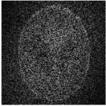
(a) $x_{\rm spec}$

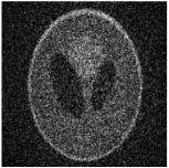
(b) $x_{\textup{t-spec}}$ ($\tau^{2}=4.6$)

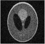
(c) $x_{\textup{null}}$ ($\gamma=0.5$)

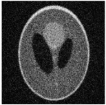
(d) $x_{\textup{null}}$ ($\gamma=0.74$)

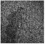
(e) $x_{\rm spec}$

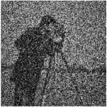
(f) $x_{\textup{t-spec}}$ ($\tau^{2}=4.1$)

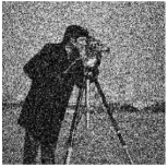
(g) $x_{\textup{null}}$ ($\gamma=0.5$)

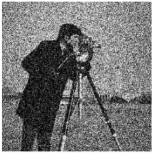
(h) $x_{\textup{null}}$ ($\gamma=0.7$)

Figure 1: Initialization with one pattern of the Phantom ((a) RE$(x_{\rm spec})=0.9604$, (b) RE$(x_{\textup{t-spec}})=0.7646$, (c) RE$(x_{\textup{null}})=0.5119$, (d) RE$(x_{\textup{null}})=0.4592$) and the Cameraman ((e) RE$(x_{\rm spec})=0.8503$, (f) RE$(x_{\textup{t-spec}})=0.7118$, (g) RE$(x_{\textup{null}})=0.4820$, (h) RE$(x_{\textup{null}})=0.4423$).

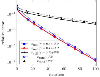
(a) Cameraman

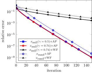
(b) Phantom

Figure 2: RE versus iteration in the one-pattern case with the (a) Cameraman and (b) Phantom. WF is tested with the optimized step size $s=$ 0.2.

(a) $|\textup{Re}(x_{\textup{t-spec}})|$ ($\tau^{2}=5$)

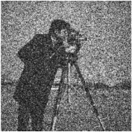
(b) $|\textup{Re}(x_{\textup{null}})|$ ($\gamma=0.5$)

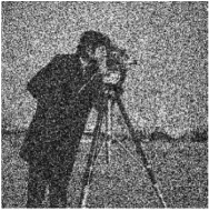
(c) $|\textup{Re}(x_{\textup{null}})|$ ($\gamma=0.63$)

(d) $|\textup{Im}(x_{\textup{t-spec}})|$ ($\tau^{2}=5$)

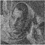
(e) $|\textup{Im}(x_{\textup{null}})|$ ($\gamma=0.5$)

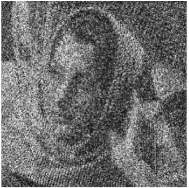
(f) $|\textup{Im}(x_{\textup{null}})|$ ($\gamma=0.63$)

(g) $|x_{\textup{t-spec}}|$ ($\tau^{2}=5$)

(h) $|x_{\textup{null}}|$ ($\gamma=0.5$)

(i) $|x_{\textup{null}}|$ ($\gamma=0.6$)

Figure 3: Initialization with two patterns for RSCB ((a)(d) RE$(x_{\textup{t-spec}})=1.3954$, (b)(e) RE$(x_{\textup{null}})=0.5736$, (c)(f) RE$(x_{\textup{null}})=0.5416$) and RPP ((g)RE$(x_{\textup{t-spec}})=1.3978$, (h) RE$(x_{\textup{null}})=0.7399$, (i) RE$(x_{\textup{null}})=0.7153$)

8.3 One-pattern experiments

Fig. 1 shows that the null vector $x_{\textup{null}}$ is more accurate than the spectral vector $x_{\rm spec}$ and the truncated spectral vector $x_{\textup{t-spec}}$ in approximating the true images. For the Cameraman (resp. the Phantom) $\hbox{\rm RR}(x_{\textup{null}})$ can be minimized by setting $\gamma\approx 0.70$ (resp. $\gamma\approx 0.74$). The optimal parameter $\tau^{2}$ for $x_{\rm t-spec}$ in (16) is about $4.1$ (resp. $4.6$).

Next we compare the performances of PAP and WF [13] with $x_{\textup{null}}$ as well as the random initialization $x_{\textup{rand}}$. Each pixel of $x_{\textup{rand}}$ is independently sampled from the uniform distribution over $[0,1]$.

To account for the real/positivity constraint, we modify (8.2) as

(102) $$W(x^{(k)}) = \left[x^{(k)}-{s^{(k)}\over\|x^{(1)}\|^{2}}\nabla F_{\rm w}(x^{(k)})\right]_{\mathcal{X}},\quad{\mathcal{X}}=\mathbb{R}^{n},\leavevmode\nobreak\ \mathbb{R}^{n}_{+}.$$

As shown in Fig. 2, the convergence of both PAP and WF is faster with $x_{\textup{null}}$ than $x_{\textup{rand}}$. In all cases, PAP converges faster than WF.

Also, the median value $\gamma=0.5$ for initialization is as good as the optimal value. The convergence of PAP with random initial condition $x_{\rm rand}$ suggests global convergence to the true object in the one-pattern case with the positivity constraint.

8.4 Two-pattern experiments

(a) RSCB

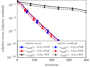
(b) RPP

Figure 4: RE and RR versus iteration for PAP and WF with two patterns. WF is tested with the optimized step size (a) $s=0.2$ and (b) $s=0.15$.

We use the complex images, RSCB and RPP, for the two-pattern simulations.

Fig. 3 shows that $x_{\rm null}$ is more accurate than the $x_{\rm spec}$ and $x_{\rm t-spec}$ in approximating $x_{0}$. The difference in RE between the initializations with the median value and the optimal values is less than $3\%$.

Fig. 4 shows that PAP outperforms WF, both with the null initialization.

As Fig. 5 shows, SAP converges much faster than PAP and takes about half the number of iterations to converge to the object. Different samples correspond to different realizations of random masks, showing robustness with respect to the ensemble of random masks. In terms of the rate of convergence, SAP with the null initialization outperforms the Fourier-domain Douglas-Rachford algorithm [19].

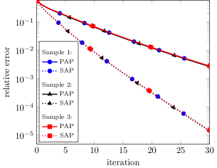
(a) RSCB

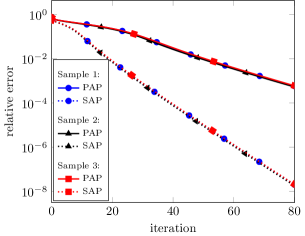
(b) RPP

Figure 5: RE versus iteration of PAP and SAP in the two-pattern case ($\gamma=0.5$).

Fig. 6 shows the RE versus iteration for the (a) one-pattern and (b) two-pattern cases. The dotted lines represent the geometric series $\{\tilde{\lambda}_{2}^{2k}\}_{k=1}^{200}$, $\{\lambda_{2}^{2k}\}_{k=1}^{200}$ and $\|{\mathcal{D}}\|_{\perp}^{k}$ (the pink line in (a) and the red and the blue lines in (b)), which track well the actual iterates (the black-solid curve in (a) and the blue- and the red-solid curves in (b)), consistent with the predictions of Theorems 5.6, 6.3 and 7.3. In particular, SAP has a better rate of convergence than PAP (0.7946 versus 0.9086).

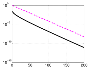
(a) One pattern: $\tilde{\lambda}^{2}_{2}=0.9084$

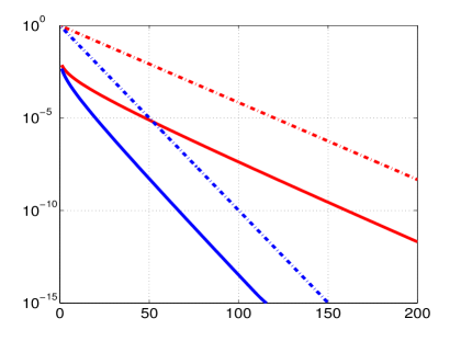
(b) SAP $\|{\mathcal{D}}\|_{\perp}=0.7946$; PAP $\lambda^{2}_{2}=0.9086$

Figure 6: RE on the log scale versus iteration with (a) one pattern and (b) two patterns (PAP in red, SAP in blue). The solid curves are the AP iterates and the dotted lines are the geometric series predicted by the theory.

8.5 Oversampling ratio

Phase retrieval with just one coded diffraction pattern without the real/positivity constraint has many solutions [28] and as a result AP with the null initialization does not perform well numerically.

What would happen if we measure two coded diffraction patterns each with fewer samples?

The amount of data in each coded diffraction pattern is measured by the oversampling ratio

$$\rho=\frac{\textup{Number of data in {\bf each} coded diffraction pattern }}{\textup{Number of image pixels}},$$

which is approximately 4 in the standard oversampling.

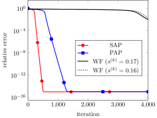
(a) RSCB ($\rho=1.65$)

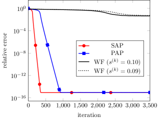
(b) RPP ($\rho=1.96$)

Figure 7: RE vs. iteration by SAP, PAP and WF with two patterns and the null initialization ($\gamma=0.38$ and $0.4$ for RSCB and RPP, respectively). The optimal step size for WF is $s=0.17$ and $0.10$ for RSCB and RPP, respectively.

For the two-pattern results in Fig. 7, we use $\rho=1.65,1.96$ (respectively for RSCB and RPP) and hence $N\approx 3.3n,3.92n$ (respectively for RSCB and RPP). For $n=256\times 256$, $3.3n\approx 216269,3.92n\approx 256901$ are both significantly less than $(2\sqrt{n}-1)^{2}=261121$, the number of data in a coded diffraction pattern with the standard oversampling.

As expected, convergence is slowed down for both methods (much less so for SAP) as the oversampling ratio decreases. Nevertheless, both SAP and PAP converge rapidly to the true solution, reaching machine precision, within 500 and 1200 iterations, while WF fails to converge within 4000 steps for RSCB and stagnates after 3000 iterations for RPP. The optimal constant step size for WF is $s=0.10$ and $0.17$ for RSCB and RPP, respectively. And if we set $s=0.11$ and $0.18$ respectively, then the relative error would blow up for both images. On the other hand, a smaller step size results in even worse performance.

8.6 Noise stability

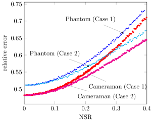
(a) One pattern

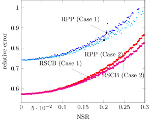
(b) Two patterns

Figure 8: RE versus NSR of the null initialization ($\gamma=0.5$)

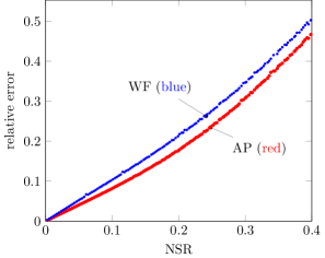
(a) Cameraman

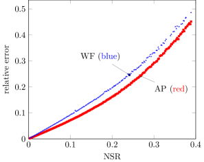
(b) Phantom

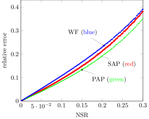
(c) RSCB

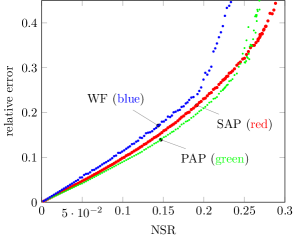
(d) RPP

Figure 9: RE versus NSR with one (top row, 500 iterations) and two (bottom row, 1000 iterations) patterns.

We test the performance of AP and WF with the Gaussian noise model where the noisy data is generated by

$$b_{\rm noisy}=|A^{*}x_{0}+\hbox{complex\ Gaussian\ noise}|.$$

The noise is measured by the Noise-to-Signal Ratio (NSR)

$$\textup{NSR}=\frac{\|b_{\rm noisy}-|A^{*}x_{0}|\|_{2}}{\|A^{*}x_{0}\|_{2}}.$$

As pointed out in Section 2.3, since the null initialization depends only on the choice of the index set $I$ and does not depend explicitly on $b$, the method is more noise-tolerant than other initialization methods.

Let $\hat{x}_{\rm null}$ be the unit leading singular vector of $A_{I_{c}}$, cf. (14). In order to compare the effect of normalization, we normalize the null vector in two different ways

(103) $$\hbox{\rm Case 1.}\quad x_{\rm null} = \alpha{\|b_{\rm noisy}\|}\cdot\hat{x}_{\rm dual}$$

(104) $$\hbox{\rm Case 2.}\quad x_{\rm null} = \alpha{\|x_{0}\|}\cdot\hat{x}_{\rm dual}$$

and then compute their respective relative errors versus NSR. As shown in Fig. 8, the slope of RE versus NSR is less than 1 in all cases. Remarkably, the slope is much smaller than 1 for small NSR when the performance curves are strictly convex and independent of the way of normalization. For large SNR ($\geq 20\%$), however, the proper normalization with $\|x_{0}\|$ (Case 2) can significantly reduce the error. The difference between the initialization errors of RPP and RSCB would disappear by and large after the AP iteration converges, see Fig. 9.

Fig. 9 shows the REs of AP and WF with the null initialization after 500 iterations for the one-pattern case and 1000 iterations for the two-pattern case. Clearly, AP consistently achieves a smaller error than WF, with a noise amplification factor slightly above 1. For RPP, WF, PAP and SAP fail to converge in 1000 steps beyond $20\%,25\%$ and $28\%$ NSR, respectively, hence the scattered data points. Increasing the maximum number of iterations can bring the upward “tails” of the curves back to roughly straightlines as in other plots.

As in Fig. 8, if $\|x_{0}\|$ is known explicitly, we can apply AP with the normalized noisy data

$$\hat{b}_{\rm noisy}=b_{\rm noisy}{\|x_{0}\|\over\|b_{\rm noisy}\|}$$

and improve the performance in Fig. 9. And the improvement is particularly significant for larger NSR. For simplicity of presentation, the results are omitted here.

9 Conclusion and discussion

Under the uniqueness framework of [28] (reviewed in Section 1.1), we have proved local geometric convergence for AP of various forms and characterized the convergence rate in terms of a spectral gap. To our knowledge, this is the only such result besides [19] for phase retrieval with one or two coded diffraction patterns. Other literature either demands a large number of coded diffraction patterns [14, 13] or asserts sublinear convergence [51]. More importantly, we have proposed and proved the null initialization to be an effective initialization method with performance guarantee comparable to, and numerical performance superior to, the spectral initialization and its truncated version [13, 11]. In practice AP with the null initialization is a globally convergent algorithm for phase retrieval with one or two coded diffraction patterns.

Of course, a positive spectral gap does not necessarily lead to a significantly sized basin of attraction for the true object. As mentioned above AP with just one coded diffraction pattern but without any object constraint still has a positive spectral gap and converges locally to the true object. However, AP with the null initialization does not perform well numerically (not shown). This is likely because the corresponding phase retrieval loses uniqueness and has many solutions [28]. On the other hand, AP with one coded diffraction pattern under the real or positivity constraint converges globally with randomly selected initial guess (Fig. 2) because the uniqueness of solution is restored with the object constraint.

This observation points to the importance of the design of measurement scheme besides the choice of algorithm (AP versus WF, e.g.). Results that do not take the measurement scheme into account (e.g. [51]) are likely to be sub-optimal in theory and practice.

A reasonable question is, How much can the measurement scheme be relaxed from that of [28]? Fig. 7 gives a tentative answer to one aspect of the question: the number of measurement data may be reduced by as much as half and still maintains a good numerical performance. Another aspect of the question is about the type of masks to be used in measurement: Indeed, besides the fine-grained (independently distributed) masks discussed in Section 1.1, the coarse-grained (correlated) masks can have a good numerical performance as well (see [29, 30]).

A shortcoming of the present work is that we are unable to provide a useful estimate for the size of the basin of attraction for AP; our current estimate is overly pessimistic (not shown). Another is that we are unable to give an error bound for AP in the case of noisy data. And finally it remains an open problem to prove global convergence of our approach (AP + the null initialization).

These questions are particularly enticing in view of superior numerical performances that strongly indicate a large basin of attraction, a high degree of noise tolerance and global convergence from randomly selected initial data.

Appendix A Proof of Theorem  2.1

The proof is based on the following two propositions.

Proposition A.1.

There exists $x_{\bot}\in\mathbb{C}^{n}$ with $x_{\bot}^{*}x_{0}=0$ and $\|x_{\bot}\|=\|x_{0}\|=1$ such that

(105) $$\frac{1}{4}\|x_{0}x_{0}^{*}-x_{\rm null}x_{\rm null}^{*}\|^{2} \leq {\|b_{I}\|^{2}\over\|A_{I}^{*}x_{\bot}\|^{2}}.$$

Proof.

Since $x_{\rm null}$ is optimally phase-adjusted, we have

(106) $$\beta:=x_{0}^{*}x_{\rm null}\geq 0$$

and

(107) $$x_{0}=\beta x_{\rm null}+\sqrt{1-\beta^{2}}\,z$$

for some unit vector $z^{*}x_{\rm null}=0$. Then

(108) $$x_{\bot}:=-(1-\beta^{2})^{1/2}x_{\rm null}+\beta z$$

is a unit vector satisfying $x_{0}^{*}x_{\perp}=0$. Since $x_{\rm null}$ is a singular vector and $z$ belongs in another singular subspace, we have

$$\|A_{I}^{*}x_{0}\|^{2} = \beta^{2}\|A_{I}^{*}x_{\rm null}\|^{2}+(1-\beta^{2})\|A_{I}^{*}z\|^{2},$$

$$\|A_{I}^{*}x_{\bot}\|^{2} = (1-\beta^{2})\|A_{I}^{*}x_{\rm null}\|^{2}+\beta^{2}\|A_{I}^{*}z\|^{2}$$

from which it follows that

$$(2-\beta^{2})\|A_{I}^{*}x_{0}\|^{2}-(1-\beta^{2})\|A_{I}^{*}x_{\bot}\|^{2}$$

$$= \|A_{I}^{*}x_{\rm null}\|^{2}+2(1-\beta^{2})^{2}\left(\|A_{I}^{*}z\|^{2}-\|A_{I}^{*}x_{\rm null}\|^{2}\right)\geq 0.$$

By (A), (17) and $\|b_{I}\|=\|A_{I}^{*}x_{0}\|$, we also have

(110) $$\frac{\|b_{I}\|^{2}}{\|A_{I}^{*}x_{\bot}\|^{2}}\geq{1-\beta^{2}\over 2-\beta^{2}}\geq{1\over 2}(1-\beta^{2})=\frac{1}{4}\|x_{0}x_{0}^{*}-x_{\rm null}x_{\rm null}^{*}\|^{2}.$$

∎

Proposition A.2.

Let $A\in\mathbb{C}^{n\times N}$ be an i.i.d. complex standard Gaussian random matrix. Then for any $\epsilon>0,\delta>0,t>0$

$$\|b_{I}\|^{2}\leq|I|\left(\left(\frac{2+t}{1-\epsilon}\right)\frac{|I|}{N}+\epsilon\left(-2\ln\left(1-{|I|\over N}\right)+\delta\right)\right)$$

with probability at least

$$1-2\exp\left(-{N}{\delta^{2}e^{-\delta}|1-\sigma|^{2}/2}\right)-2\exp\left(-{2\epsilon^{2}|1-\sigma|^{2}}\sigma^{2}N\right)-Q$$

where $Q$ has the asymptotic upper bound

$$2\exp\left\{-c\min\left[{e^{2}t^{2}\over 16}{|I|^{2}\over N}\left(\ln\sigma^{-1}\right)^{2},\leavevmode\nobreak\ {et\over 4}|I|\ln\sigma^{-1}\right]\right\},\quad\sigma:={|I|\over N}\ll 1.$$

The proof of Proposition A.2 is given in the next section.

Now we turn to the proof of Theorem 2.1.

Without loss of the generality we may assume $\|x_{0}\|=1$. Otherwise, we replace $x_{0},x_{null}$ by $x_{0}/\|x_{0}\|$ and $x_{\rm null}/\|x_{0}\|$, respectively. By an additional orthogonal transformation which does not affect the statistical nature of the complex Gaussian matrix, we can map $x_{0}$ to $e_{1}$, the canonical vector with 1 as the first entry and zero elsewhere.

Let $x_{\bot}$ be any unit vector of the form $x_{\bot}=[0,y^{\top}]^{\top}$ where $y\in\mathbb{C}^{n-1}$ is an unit vector. Let $A^{\prime}\in\mathbb{C}^{N\times(n-1)}$ be the sub-column matrix of $A_{I}^{*}$ with its first column vector deleted and $\{\nu_{i}\}_{i=1}^{n-1}$ the singular values of $A^{\prime}$ in the ascending order. Let

$$B^{\prime}=A^{\prime}\,\mathop{\operator@font diag}\nolimits(y/|y|)$$

which has the same singular values as $A^{\prime}$. We have

$$\|A_{I}^{*}x_{\bot}\|=\|B^{\prime}\,|y|\|$$

and hence

$$\|A_{I}^{*}x_{\bot}\|=(\|\Re(B^{\prime})\,|y|\|^{2}+\|\Im(B^{\prime})\,|y|\|^{2})^{1/2}\geq\sqrt{2}\left(\|\Re(B^{\prime})\,|y|\|\wedge\|\Im(B^{\prime})\,|y|\|\right).$$

Note that $A^{\prime}$ and $B^{\prime}$ are both i.i.d. complex Gaussian random matrices for any fixed $y\in\mathbb{C}^{n-1}$. By the theory of Wishart matrices [23], the singular values $\{\nu_{j}^{R}\}_{j=1}^{n-1},\{\nu_{j}^{I}\}_{j=1}^{n-1}$ (in the ascending order) of $\Re(B^{\prime}),\Im(B^{\prime})$ satisfy the probability bounds that for every $t>0$ and $j=1,\cdots,n-1$

(111) $$\mathbb{P}\left(\sqrt{|I|}-(1+t)\sqrt{n}\leq\nu_{j}^{R}\leq\sqrt{|I|}+(1+t)\sqrt{n}\right) \geq 1-2e^{-nt^{2}/2},$$

(112) $$\mathbb{P}\left(\sqrt{|I|}-(1+t)\sqrt{n}\leq\nu_{j}^{I}\leq\sqrt{|I|}+(1+t)\sqrt{n}\right) \geq 1-2e^{-nt^{2}/2}.$$

By Proposition A.1 and (111)-(112), we have

$$\|x_{0}x_{0}^{*}-x_{\rm null}x_{\rm null}^{*}\| \leq {\sqrt{2}\|b_{I}\|\over\|\Re(B^{\prime})\,|y|\|\wedge\|\Im(B^{\prime})\,|y|\|}$$

$$\leq \sqrt{2}\|b_{I}\|(\nu^{R}_{n-1}\wedge\nu^{I}_{n-1})^{-1}$$

$$\leq \sqrt{2}\|b_{I}\|(\sqrt{|I|}-(1+t)\sqrt{n})^{-1}.$$

By Proposition A.2, we obtain the desired bound (19). The success probability is at least the expression (A.2) minus $4e^{-nt^{2}/2}$ which equals the expression (20).

A.1 Proof of Proposition A.2

By the Gaussian assumption, $b(i)^{2}=|a_{i}^{*}x_{0}|^{2}$ has a chi-squared distribution with the probability density $e^{-z/2}/2$ on $z\in[0,\infty)$ and the cumulative distribution

$$F(\tau):=\int_{0}^{\tau}2^{-1}\exp(-z/2)dz=1-\exp(-\tau/2).$$

Let

(113) $$\tau_{*}=-2\ln(1-|I|/N)$$

for which $F(\tau_{*})=|I|/N.$

Define

$$\hat{I}:=\{i:b(i)^{2}\leq\tau_{*}\}=\{i:F(b^{2}(i))\leq|I|/N\},$$

and

$$\|\hat{b}\|^{2}:=\sum_{i\in\hat{I}}b(i)^{2}.$$

Let

$$\{\tau_{1}\leq\tau_{2}\leq\ldots\leq\tau_{N}\}$$

be the sorted sequence of $\{b(1)^{2},\ldots,b(N)^{2}\}$ in magnitude.

Proposition A.3.

(i) For any $\delta>0$, we have

(114) $$\tau_{|I|} \leq \tau_{*}+\delta$$

with probability at least

(115) $$1-\exp\left(-\frac{N}{2}{\delta^{2}e^{-\delta}|1-{{|I|/N}}|^{2}}\right)$$

(ii) For each $\epsilon>0$, we have

(116) $$|\hat{I}|\geq|I|(1-\epsilon)$$

or equivalently,

(117) $$\tau_{\lfloor|I|(1-\epsilon)\rfloor}\leq\tau_{*}$$

with probability at least

(118) $$1-2\exp\left(-{4\epsilon^{2}|1-{|I|/N}|^{2}}|I|^{2}/N\right)$$

Proof.

(i) Since $F^{\prime}(\tau)=\exp(-\tau/2)/2$,

(119) $$|F(\tau+\epsilon)-F(\tau)|\geq\epsilon/2\exp(-(\tau+\epsilon)/2).$$

For $\delta>0$, let

$$\zeta:=F(\tau_{*}+\delta)-F(\tau_{*})$$

which by (119) satisfies

(120) $$\zeta\geq\frac{\delta}{2}\exp(-\frac{1}{2}(\tau_{*}+\delta)).$$

Let $\{w_{i}:i=1,\ldots,N\}$ be the i.i.d. indicator random variables

$$w_{i}=\chi_{\{b(i)^{2}>\tau_{*}+\delta\}}$$

whose expectation is given by

$$\mathbb{E}[w_{i}]=1-F(\tau_{*}+\delta).$$

The Hoeffding inequality yields

$$\mathbb{P}(\tau_{|I|}>\tau_{*}+\delta) = \mathbb{P}\left(\sum_{i=1}^{N}w_{i}>N-|I|\right)$$

$$= \mathbb{P}\left(N^{-1}\sum_{i=1}^{N}w_{i}-\mathbb{E}[w_{i}]>1-|I|/N-\mathbb{E}[w_{i}]\right)$$

$$= \mathbb{P}\left(N^{-1}\sum_{i=1}^{N}w_{i}-\mathbb{E}[w_{i}]>\zeta\right)$$

$$\leq \exp(-2N\zeta^{2}).$$

Hence, for any fixed $\delta>0$,

(122) $$\tau_{|I|}\leq \tau_{*}+\delta$$

holds with probability at least

$$1-\exp(-2N\zeta^{2}) \geq 1-\exp\left(-\frac{N\delta^{2}}{2}e^{-\tau_{*}-\delta}\right)$$

$$= 1-\exp\left(-\frac{N\delta^{2}}{2}e^{-\delta}\left|1-{|I|/N}\right|^{2}\right)$$

by (120).

(ii) Consider the following replacement

$$\begin{array}[]{cl}(a)&|I|\longrightarrow\lceil|I|(1-\epsilon)\rceil\\ (b)&\tau_{*}\longrightarrow F^{-1}(\lceil|I|(1-\epsilon)\rceil/N)\\ (c)&\delta\longrightarrow F^{-1}(|I|/N)-F^{-1}(\lceil|I|(1-\epsilon)\rceil/N)\\ (d)&\zeta\longrightarrow F^{-1}(\tau_{*}+\delta)-F^{-1}(\tau_{*})=|I|/N-\lceil|I|(1-\epsilon)\rceil/N=\frac{\lfloor|I|\epsilon\rfloor}{N}\end{array}$$

in the preceding argument. Then (A.1) becomes

$$\mathbb{P}\left(\tau_{\lceil|I|(1-\epsilon)\rceil}>F^{-1}(|I|/N)\right) \leq \exp(-2N\zeta^{2})=\exp\left(-\frac{2\lfloor|I|\epsilon\rfloor^{2}}{N}\right).$$

That is,

$$\tau_{\lceil|I|(1-\epsilon)\rceil}\leq\tau_{*}$$

holds with probability at least

$$1-\exp(-2{\lfloor|I|\epsilon\rfloor^{2}}/{N}).$$

∎

Proposition A.4.

For each $\epsilon>0$ and $\delta>0$,

(123) $$\frac{\|b_{I}\|^{2}}{|I|}\leq\frac{\|\hat{b}\|^{2}}{|\hat{I}|}+\epsilon(\tau_{*}+\delta)$$

with probability at least

(124) $$1-2\exp\left(-\frac{1}{2}{\delta^{2}e^{-\delta}|1-{|I|/N}|^{2}N}\right)-2\exp\left(-{2\epsilon^{2}|1-{|I|/N}|^{2}}{|I|^{2}\over N}\right).$$

Proof.

Since $\{\tau_{j}\}$ is an increasing sequence, the function $T(m)=m^{-1}\sum_{i=1}^{m}\tau_{i}$ is also increasing. Consider the two alternatives either $|I|\geq|\hat{I}|$ or $|\hat{I}|\geq|I|$. For the latter,

$${\|b_{I}\|^{2}}/{|I|}\leq{\|\hat{b}\|^{2}}/{|\hat{I}|}$$

due to the monotonicity of $T$.

For the former case $|I|\geq|\hat{I}|$, we have

$$T(|I|) = |I|^{-1}\sum_{i=1}^{|\hat{I}|}\tau_{i}+|I|^{-1}\sum_{i=|\hat{I}|+1}^{|I|}\tau_{i}$$

$$\leq T(|\hat{I}|)+|I|^{-1}(|I|-|\hat{I}|)\tau_{|I|}.$$

By Proposition A.3 (ii) $|\hat{I}|\geq(1-\epsilon)|I|$ and hence

$$T(|I|) \leq T(|\hat{I}|)+|I|^{-1}(|I|-|I|(1-\epsilon))\tau_{|I|}=T(|\hat{I}|)+\epsilon\tau_{|I|}$$

with probability at least given by (118).

By Proposition A.3 (i), $\tau_{|I|}\leq\tau_{*}+\delta$ with probability at least given by (115). ∎

Continuing the proof of Proposition A.2, let us consider the i.i.d. centered, bounded random variables

(125) $$Z_{i}:={N^{2}\over|I|^{2}}\left[b(i)^{2}\chi_{\tau_{*}}-\mathbb{E}[b(i)^{2}\chi_{\tau_{*}}]\right]$$

where $\chi_{\tau_{*}}$ is the characteristic function of the set $\{b(i)^{2}\leq\tau_{*}\}$. Note that

(126) $$\mathbb{E}(b(j)^{2}\chi_{\tau_{*}}) = \int_{0}^{\tau_{*}}2^{-1}z\exp(-z/2)dz=2-(\tau_{*}+2)\exp(-\tau_{*}/2)\leq 2|I|^{2}/N^{2}$$

and hence

(127) $$-2\leq Z_{i}\leq\sup\left\{{N^{2}\over|I|^{2}}b(i)^{2}\chi_{\tau_{*}}\right\}={N^{2}\over|I|^{2}}\tau_{*}.$$

Next recall the Bernstein-inequality.

Proposition A.5.

[57] Let $Z_{1},\ldots,Z_{N}$ be i.i.d. centered sub-exponential random variables. Then for every $t\geq 0$, we have

(128) $$\mathbb{P}\left\{N^{-1}|\sum_{i=1}^{N}Z_{i}|\geq t\right\}\leq 2\exp\left\{-c\min(Nt^{2}/K^{2},Nt/K)\right\},$$

where $c$ is an absolute constant and

$$K=\sup_{p\geq 1}p^{-1}(\mathbb{E}|Z_{j}|^{p})^{1/p}.$$

Remark A.6.

For $K$ we have the following estimates

$$K \leq {2N^{2}\over|I|^{2}}\sup_{p\geq 1}p^{-1}(\mathbb{E}|b(i)^{2}\chi_{\tau_{*}}|^{p})^{1/p}$$

$$\leq {2N^{2}\over|I|^{2}}\tau_{*}\sup_{p\geq 1}p^{-1}(\mathbb{E}\chi_{\tau_{*}})^{1/p}$$

$$\leq {2N^{2}\over|I|^{2}}\tau_{*}\sup_{p\geq 1}p^{-1}(1-e^{-\tau_{*}/2})^{1/p}.$$

The maximum of the right hand side of (A.6) occurs at

$$p_{*}=-\ln(1-e^{-\tau_{*}/2})$$

and hence

$$K \leq {2N^{2}\over|I|^{2}}{\tau_{*}\over p_{*}}(1-e^{-\tau_{*}/2})^{1/p_{*}}.$$

We are interested in the regime

$$\tau_{*}\asymp 2|I|/N\ll 1$$

which implies

$$p_{*}\asymp-\ln{\tau_{*}\over 2}\asymp\ln{N\over|I|}$$

and consequently

(130) $$K\leq{4N\over e|I|}\left(\ln{N\over|I|}\right)^{-1},\quad\sigma=|I|/N\ll 1.$$

On the other hand, upon substituting the asymptotic bound (130) in the probability bound

$$Q=2\exp\left\{-c\min(Nt^{2}/K^{2},Nt/K)\right\}$$

of (128), we have

$$K\leq 2\exp\left\{-c\min\left[{e^{2}t^{2}\over 16}\left(\ln\sigma^{-1}\right)^{2}{|I|^{2}/N},\leavevmode\nobreak\ {et\over 4}|I|\ln\sigma^{-1}\right]\right\},\quad\sigma\ll 1.\\$$

The Bernstein inequality ensures that with high probability

$$\left|{\|\hat{b}\|^{2}\over N}-\mathbb{E}(b^{2}(i)\chi_{\tau_{*}})\right|\leq t{|I|^{2}\over N^{2}}.$$

By (116) and (126), we also have

$$\frac{\|\hat{b}\|^{2}}{|\hat{I}|} \leq \mathbb{E}(b(i)^{2}\chi_{\tau_{*}})\frac{N}{|\hat{I}|}+t\frac{|I|^{2}}{|\hat{I}|N}$$

$$\leq \left(\mathbb{E}(b(i)^{2}\chi_{\tau_{*}})\frac{N^{2}}{|I|^{2}}+t\right)\frac{|I|}{N}$$

$$\leq \frac{2+t}{1-\epsilon}\cdot\frac{|I|}{N}$$

By Prop. A.4, we now have

$$\|b_{I}\|^{2} \leq |I|\left({\|\hat{b}\|^{2}\over|\hat{I}|}+\epsilon\left(\tau_{*}+\delta\right)\right)$$

with probability at least given by (20), which together with (A.1) and (113) complete the proof of Proposition A.2.

Acknowledgements. We thank anonymous referees for helpful suggestions that lead to improvement of the original manuscript.

References

- [1] R. Balan, B. G. Bodmann , P. G. Casazza and D. Edidin, “Painless reconstruction from magnitudes of frame coefficients,” J Fourier Anal Appl 15, 488-501 (2009).
- [2] R. Balan, P. Casazza and D. Edidin, “On signal reconstruction without phase,” Appl. Comput. Harmon. Anal. 20, 345-356 (2006).
- [3] R. Balan, Y. Wang, “Invertibility and robustness of phaseless reconstruction”, arXiv preprint, arXiv:1308.4718, 2013.
- [4] A. S. Bandeira, J. Cahill, D. G. Mixon, A. A. Nelson, “ Saving phase: Injectivity and stability for phase retrieval,” Appl. Comput. Harmon. Anal. 37, 106-125 (2014).
- [5] A. S. Bandeira, Y. Chen and D. Mixon, “Phase retrieval from power spectra of masked signals,” Inform. Infer. (2014) 1-20.
- [6] H.H. Bauschke and J. Borwein, “On projection algorithms for solving convex feasibility problems,” SIAM Review 38, 367-426 (1996).
- [7] H.H. Bauschke, P.L. Combettes and D. R. Luke, “Phase retrieval, error reduction algorithm, and Fienup variants: a view from convex optimization,” J. Opt. Soc. Am. A 19, 13341-1345 (2002).
- [8] H. H. Bauschke, P. L. Combettes, and D. R. Luke, “Finding best approximation pairs relative to two closed convex sets in Hilbert spaces,” J. Approx. Th. 127, 178-192 (2004).
- [9] D. P. Bertsekas. Nonlinear programming. Athena scientific, 2003.
- [10] L.M. Bregman, “The method of successive projection for finding a common point of convex sets,” Soviet Math. Dokl. 162, 688-692 (1965).
- [11] E.J. Candès and Y. Chen, “ Solving random quadratic systems of equations is nearly as easy as solving linear systems.” arXiv:1505.05114, 2015.
- [12] E.J. Candès, Y.C. Eldar, T. Strohmer, and V. Voroninski, “Phase retrieval via matrix completion,” SIAM J. Imaging Sci. 6, 199-225 (2013).
- [13] E.J. Candes, X. Li and M. Soltanolkotabi, “Phase retrieval via Wirtinger flow: theory and algorithms,” IEEE Trans Inform. Th. 61(4), 1985–2007 (2015).
- [14] E.J. Candes, X. Li and M. Soltanolkotabi. “Phase retrieval from coded diffraction patterns.” Appl. Comput. Harmon. Anal. 39, 277-299 (2015).
- [15] E.J. Candès, T. Strohmer, and V. Voroninski, “ Phaselift: exact and stable signal recovery from magnitude measurements via convex programming,” Comm. Pure Appl. Math. 66, 1241-1274 (2012).
- [16] A. Chai, M. Moscoso, G. Papanicolaou, “Array imaging using intensity-only measurements,” Inverse Problems 27 (1) (2011).
- [17] H.N. Chapman et al. “Femtosecond X-ray protein nanocrystallography”. Nature 470, 73-77 (2011).
- [18] H.N. Chapman, C. Caleman and N. Timneanu, “Diffraction before destruction,” Phil. Trans. R. Soc. B 369 20130313 (2014).
- [19] P. Chen and A. Fannjiang, “Phase retrieval with a single mask by the Douglas-Rachford algorithm,” arXiv:1509.00888.
- [20] W. Cheney and A. Goldstein, “Proximity maps for convex sets,” Proc. Amer. Math. Soc. 10, 448-450 (1959).
- [21] G. Cimmino, “Calcolo approssimato per le soluzioni dei sistemi di equazioni lineari,” Ric. Sci. Progr. Tecn. Econom. Naz. 16 326-333 (1938).
- [22] A. Conca, D. Edidin, M. Hering, and C. Vinzant, “An algebraic characterization of injectivity in phase retrieval,” Appl. Comput. Harmon. Anal. 38 346-356 (2015).
- [23] K.R. Davidson and S.J. Szarek. “Local operator theory, random matrices and Banach spaces,” in Handbook of the geometry of Banach spaces, Vol. I, pp. 317-366. Amsterdam: North-Holland, 2001.
- [24] L. Demanet and P. Hand, “Stable optimizationless recovery from phaseless linear measurements,” J. Fourier Anal. Appl. 20, 199-221 (2014).
- [25] F. Deutsch. Best Approximation in Inner Product Spaces, Springer, New York, 2001.
- [26] D.C. Dobson, “ Phase reconstruction via nonlinear least-squares,” Inverse Problems8 (1992) 541-557.
- [27] Y.C. Eldar and S. Mendelson, “Phase retrieval: Stability and recovery guarantees,” Appl. Comput. Harmon. Anal. 36, pp. 473-494 (2014).
- [28] A. Fannjiang, “Absolute uniqueness of phase retrieval with random illumination,” Inverse Problems 28, 075008 (2012).
- [29] A. Fannjiang and W. Liao, “Phase retrieval with random phase illumination,” J. Opt. Soc. A 29, 1847-1859 (2012).
- [30] A. Fannjiang and W. Liao, “Fourier phasing with phase-uncertain mask,” Inverse Problems 29 125001 (2013).
- [31] J. R. Fienup, “Phase retrieval algorithms: a comparison,” Appl. Opt. 21, 2758-2769 (1982).
- [32] J.R. Fienup, “Phase retrieval algorithms: a personal tour ”, Appl. Opt. 52 45-56 (2013).
- [33] R.W. Gerchberg and W. O. Saxton, “A practical algorithm for the determination of the phase from image and diffraction plane pictures,” Optik 35, 237-246 (1972).
- [34] A.A. Goldstein. “ Convex programming in Hilbert space.” Bull. Am. Math. Soc. 70, 709-710 (1964).
- [35] D. Gross, F. Krahmer and R. Kueng, “A partial derandomization of phaselift using spherical designs”, arXiv:1310.2267, 2013.
- [36] M. Hayes,“The reconstruction of a multidimensional sequence from the phase or magnitude of its Fourier transform,” IEEE Trans. Acoust. Speech Signal Process 30, 140-154 (1982).
- [37] R. Hesse, D. R. Luke, S. Sabach, and M.K. Tam, “Proximal heterogeneous block implicit-explicit method and application to blind ptychographic diffraction imaging,” SIAM J. Imag. Sci. 8 pp. 426-457 (2015).
- [38] S. Kaczmarz, “Angenäherte Auflösung von Systemen linearer Gleichungen,” Bull. Internat. Acad. Pol. Sci. Lett. Ser. A 35, 355-357 (1937).
- [39] M.K. Klibanov, “On the recovery of a 2-D function from the modulus of its Fourier transform,” J. Math. Anal. Appl. 323 818-843 (2006).
- [40] M.K. Klibanov, “Uniqueness of two phaseless non-overdetermined inverse acoustics problems in 3-d,”Appl. Anal. 93 1135-1149 (2013).
- [41] E.S. Levitin and B.T. Poljak, “Constrained minimization methods.” U.S.S.R. Comput. Math. Math. Phys. 6, 1-50 (1965).
- [42] A.S. Lewis , D.R. Luke and J. Malick, “Local linear convergence for alternating and averaged nonconvex projections,” Found. Comput. Math. 9(4), 485–513 (2009)
- [43] X. Li, V. Voroninski, “Sparse signal recovery from quadratic measurements via convex programming,” SIAM J. Math. Anal. 45 (5), 3019-3033 (2013).
- [44] S. Marchesini, “ A unified evaluation of iterative projection algorithms for phase retrieval,” Rev. Sci. Instr. 78, 011301 (2007).
- [45] J. Miao, J. Kirz and D. Sayre, “The oversampling phasing method,” Acta Cryst. D 56, 1312–1315 (2000).
- [46] J. Miao, D. Sayre and H.N. Chapman, “Phase retrieval from the magnitude of the Fourier transforms of nonperiodic objects,” J. Opt. Soc. Am. A 15 1662-1669 (1998).
- [47] A. Migukin, V. Katkovnik and J. Astola, “Wave field reconstruction from multiple plane intensity-only data: augmented Lagrangian algorithm,” J. Opt. Soc. Am. A 28, 993-1002 (2011).
- [48] P. Netrapalli, P. Jain, S. Sanghavi, “Phase retrieval using alternating minimization,” arXiv:1306.0160v2, 2015.
- [49] J. von Neuman, Functional Operators Vol. II. The Geometry of Orthogonal Spaces. Annals of Math. Studies 22. Princeton University Press, 1950. Reprint of notes distributed in 1933.
- [50] R. Neutze, R. Wouts, D. van der Spoel, E. Weckert, J. Hajdu, “Potential for biomolecular imaging with femtosecond x-ray pulses,” Nature 406 753-757 (2000).
- [51] D. Noll and A. Rondepierre, “On local convergence of the method of alternating projections,” Found. Comput. Math. 16, pp 425-455 (2016).
- [52] H. Ohlsson, A.Y. Yang, R. Dong and S.S. Sastry, “Compressive phase retrieval from squared output measurements via semidefinite programming,” arXiv:1111.6323, 2011.
- [53] J. Ranieri, A. Chebira, Y.M. Lu, M. Vetterli, “Phase retrieval for sparse signals: uniqueness conditions,” arXiv:1308.3058, 2013.
- [54] H.A. Schwarz, “Ueber einen Grenzũbergang durch alternirendes Verfahren,” Vierteljahrsschrift der Naturforschenden Gessellschaft in Zurich 15, 272-286 (1870).
- [55] Y. Shechtman, Y.C. Eldar, O. Cohen, H.N. Chapman, M. Jianwei and M. Segev, “Phase retrieval with application to optical imaging: A contemporary overview,” IEEE Mag. Signal Proc. 32(3) (2015), 87 - 109.
- [56] M.M. Seibert et. al “Single mimivirus particles intercepted and imaged with an X-ray laser.” Nature 470, U78-U86 (2011).
- [57] R. Vershynin. “Introduction to the non-asymptotic analysis of random matrices.” arXiv preprint arXiv:1011.3027.
- [58] I. Waldspurger, A. d’Aspremont and S. Mallat, “Phase recovery, maxCut and complex semidefinite programming,” arXiv:1206.0102.
- [59] Z. Wen, C. Yang, X. Liu and S. Marchesini, “Alternating direction methods for classical and ptychographic phase retrieval,” Inverse Problems 28, 115010 (2012).
- [60] P. Yin and J. Xin, “Phaseliftoff: an accurate and stable phase retrieval method based on difference of trace and Frobenius norms,” Commun. Math. Sci. 13 (2015).