Finite volume element method for two-dimensional fractional subdiffusion problems

Abstract

In this paper, a semi-discrete spatial finite volume (FV) method is proposed and analyzed for approximating solutions of anomalous subdiffusion equations involving a temporal fractional derivative of order $\alpha\in(0,1)$ in a two-dimensional convex polygonal domain. Optimal error estimates in $L^{\infty}(L^{2})$- norm is shown to hold. Superconvergence result is proved and as a consequence, it is established that quasi-optimal order of convergence in $L^{\infty}(L^{\infty})$ holds. We also consider a fully discrete scheme that employs FV method in space, and a piecewise linear discontinuous Galerkin method to discretize in temporal direction. It is, further, shown that convergence rate is of order $O(h^{2}+k^{1+\alpha}),$ where $h$ denotes the space discretizing parameter and $k$ represents the temporal discretizing parameter. Numerical experiments indicate optimal convergence rates in both time and space, and also illustrate that the imposed regularity assumptions are pessimistic. Fractional diffusion equation, finite volume element, discontinuous Galerkin method, variable meshes, convergence analysis

1 Introduction

Let $\Omega$ be a bounded, convex polygonal domain in $\mathbb{R}^{2}$ with boundary $\partial\Omega$, and let $f$ and $u_{0}$ be given functions defined on their respective domains. Consider the subdiffusion equation:

$$u^{\prime}(x,t)+\mathcal{B}^{\alpha}\mathcal{L}u(x,t)=f(x,t) \quad\mbox{ in }\Omega\times(0,T],$$ (1a)

$$u(x,t)=0 \quad\mbox{ on }\partial\Omega\times(0,T],$$ (1b)

$$u(x,0)=u_{0}(x) \quad\mbox{ in }\Omega,$$ (1c)

where $\mathcal{L}u=-\Delta u$, $u^{\prime}$ is the partial derivative of $u$ with respect to time, $\mathcal{B}^{\alpha}:={{}^{R}}{\rm D}^{1-\alpha}$ is the Riemann–Liouville fractional derivative in time defined by: for $0<\alpha<1$,

$$\mathcal{B}^{\alpha}\varphi(t):=\frac{\partial}{\partial t}\mathcal{I}^{\alpha}\varphi(t):=\frac{\partial}{\partial t}\int_{0}^{t}\omega_{\alpha}(t-s)\varphi(s)\,ds\quad\text{with}\quad\omega_{\alpha}(t):=\frac{t^{\alpha-1}}{\Gamma(\alpha)}$$ (2)

with $\mathcal{I}^{\alpha}$ being the temporal Riemann–Liouville fractional integral operator of order $\alpha$.

Fractional diffusion models received considerable attention over the last two decades from both practical and theoretical point of view. Researchers have found numerous porous media systems in which some key underlying random motion conform to a model where the diffusion is not classical, it is instead anomalously slow (fractional subdiffusion) or fast (super-diffusion). For example, the fractional diffusion problem (1) captures the dynamics of some subdiffusion processes, where the growth of the mean square displacement is slower compared to a Gaussian process, see Podlubny (1999) for more detail. The modeling of this problem is actually based on continuous time random walks and master equations with power law waiting time densities (Henry & Wearne (2000)), where $u$ represents the probability density function for finding a particle at location $x$ and at time $t$ (with waiting time and the jumps that are statistically independent). Fractional diffusion models have been successfully used to describe diffusion in several phenomena including media with fractal geometry (Nigmatulin (1986)), highly heterogeneous aquifer (Adams & Gelhar (1992)), and underground environmental problem (Hatano & Hatano (1998)).

Many authors have proposed various techniques for approximating the solution $u$ of (1), however obtaining sharp error bounds under reasonable regularity assumptions on $u$ has proved challenging. Several types of finite difference schemes (implicit and explicit) were investigated; see Chen et al. (2012), Cuesta et al. (2006), Cui (2009), Langlands & Henry (2005), Mustapha (2011), Quintana-Murillo & Yuste (2013), Zhang et al. (2014) and related reference, therein. The error analyses in most of these papers typically assume that the solution $u$ is sufficiently smooth, including at $t=0$. This enforces imposing compatibility conditions on the given data. In earlier works on time-stepping discontinuous Galerkin (DG) method (including $hp$-versions) combined with spatial standard Galerkin method by the second author and McLean (McLean & Mustapha (2009, 2015), Mustapha (2015), Mustapha & McLean (2013)), unbounded time derivatives of $u$ as $t\to 0$ was allowed (which is typically the case) in the error analysis, also the case of non-smooth initial data was included. Variable time steps were employed to compensate the singular behavior of $u$, and consequently maintain optimal order rates of convergence.

Our main aim is to propose and analyze a method using exact integration in time and finite volume (FV) method for the space discretization for the two-dimensional fractional model (1). Then, we combine the FV scheme in space with a piecewise-linear time-stepping DG scheme which will then define a fully-discrete scheme. Compared to finite differences and finite elements, FV method is easier to implement on structured as well as unstructured meshes and offers flexibility in tackling domains with complex boundaries. Further, it ensures local conservation property of the fluxes which makes this method more attractive in applications. The approach followed here is to formulate the problem in the Petrov-Galekin frame using two different meshes to define the trial space and test space, see Bank & Rose (1987), Cai (1991) and Süli (1991) for some earlier results in this direction. This frame work helps us to derive error estimates which are similar in spirit to tools developed for the error analysis of finite element method. The choice of the FV method for the problem under consideration is as used in Chatzipantelidis et al. (2004), Ewing et al. (2000), and Chou & Li (2000).

The major contribution of the present article can be summarized as follows. We first prove that, under certain regularity assumptions on $u$ of problem (1), the error of the FV approximation to the solution $u$ in the $L^{\infty}(L^{2})$-norm (that is, $L^{\infty}\bigr{(}0,T;L^{2}(\Omega)\bigr{)}$-norm) converge with order $h^{2}$, where $h$ is the maximum diameter of the elements of the spatial mesh; see Theorem 4.1. The imposed regularity conditions on $u$ can be satisfied by imposing some compatibility conditions on the given data taking into consideration that the derivative of $u$ is not bounded near $t=0$, see the discussion after Theorem 4.1. In addition, under more restrictive regularity assumptions, we show errors of order $h^{2}$ in the stronger $L^{\infty}(L^{\infty})$-norm, see Theorem 4.7. Since in the limiting case $\alpha\to 0$ the problem (1) reduces to the classical heat problem, these convergence results extend those obtained in Chatzipantelidis et al. (2004, 2009) and Chou & Li (2000) for the heat equation. This extension is indeed not straightforward, we make the full use of several important properties of the fractional derivative operator and also use clever steps (see for instance the proof of Lemma 4.5) to achieve our goal. In the second part of the paper, we derive the error from the fully-discrete scheme (DG in time and FV in space) for (1). In the $L^{\infty}(L^{2})$-norm, we show convergence of order $h^{2}+k^{1+\alpha}$ (that is, suboptimal in time) where $k$ is the maximum time step-size. Proving this rate of convergence in the stronger $L^{\infty}(L^{\infty})$-norm is beyond the scope of the paper due to several technical difficulties. It is worthy to mention that the numerical results demonstrate optimal convergence rate in both time and space in the $L^{\infty}(L^{\infty})$-norm, and also shows that the regularity conditions on $u$ are pessimistic. In this regard, the approach used in the time-stepping DG error analysis in Mustapha (2015) might be beneficial to prove a better convergence rate in time, $k^{\frac{3+\alpha}{2}}$ instead of $k^{1+\alpha}$.

An outline of the paper is as follows. In the next section, we introduce some notations and state some important properties of the time fractional operator $\mathcal{B}^{\alpha}$. In Section 3, we introduce our semi-discrete FV scheme in space for problem (1) and define some interpolation operators that play an important role in our error analysis. Section 4 is devoted to prove the main convergence result from the FV discretization, Theorems 4.1 and 4.7. Particularly relevant to this a priori error analysis is the appropriate use of several important properties of the operator $\mathcal{B}^{\alpha}$. In Section 5, we define our fully-discrete DG FV scheme and show the corresponding convergence results in the following section, see Theorem 6.3. Finally, in Section 6, we present some numerical results to demonstrate our theoretical achievements and illustrate optimal rates of convergence in both time and space (not only in space as the theory suggested) in the $L^{\infty}(L^{\infty})$-norm under weaker regularity assumptions than the theory required.

2 Notation and Preliminaries.

Denote by $(\cdot,\cdot)$ and $\|\cdot\|$ the $L^{2}$-inner product and its induced norm on $L^{2}(\Omega)$, respectively. The $L^{\infty}(\Omega)$-norm is denoted by $\|\cdot\|_{\infty}$. Let $H^{m}(\Omega)=W^{m,2}(\Omega)$ denote the standard Sobolev space equipped with the usual norm $\|\cdot\|_{m}$. With $H_{0}^{1}(\Omega)=\{v\in H^{1}(\Omega):v=0\;\mbox{on}\;\partial\Omega\},$ let $A(\cdot,\cdot):H_{0}^{1}(\Omega)\times H_{0}^{1}(\Omega)\rightarrow\mathbb{R}$ be the bilinear form associated with the operator $\mathcal{L}$ which is symmetric and positive definite on $H_{0}^{1}(\Omega)$. Then, the weak formulation for (1) is to seek $u:(0,T]\longrightarrow H^{1}_{0}(\Omega)$ such that

$$(u^{\prime},v)+A(\mathcal{B}^{\alpha}u,v)=(f,v)\quad\forall~{}v\in H_{0}^{1}(\Omega)\quad{with}~{}~{}u(0)=u_{0}.$$ (1)

Note that for $\varphi\in W^{1,1}(0,T)$, $\mathcal{B}^{\alpha}$ satisfies the following property (Theorem A.1, McLean (2012)):

$$\int_{0}^{T}\mathcal{B}^{\alpha}\varphi(t)\,\varphi(t)\,dt\geq c_{\alpha}T^{\alpha-1}\int_{0}^{T}|\varphi(t)|^{2}\,dt\;\;\;\mbox{ for }\;0<\alpha<1,$$

where $c_{\alpha}=\pi^{1-\alpha}(1-\alpha)^{1-\alpha}(2-\alpha)^{\alpha-2}\sin(\alpha\pi/2)$ is a positive constant.

In contrast, the Riemann–Liouville operator $\mathcal{I}^{\alpha}$ has also some positivity property but with a weaker lower bound compared to the one of the operator $\mathcal{B}^{\alpha}.$ More precisely, by Lemma 3.1(ii) in Mustapha & Schötzau (2014), it follows that for piecewise continuous functions $\varphi:[0,T]\to\mathbb{R},$

$$\int_{0}^{T}\mathcal{I}^{\alpha}\varphi(t)\,\varphi(t)\,dt\geq\cos(\alpha\pi/2)\int_{0}^{T}|\mathcal{I}^{\alpha/2}\varphi(t)|^{2}\,dt\geq 0~{}~{}{\rm for}~{}~{}0<\alpha<1\,.$$ (2)

Since the bilinear form $A(\cdot,\cdot)$ is symmetric positive definite, the following holds: for $W^{1,1}(0,T;H_{0}^{1}(\Omega))$,

$$\int_{0}^{T}A(\mathcal{B}^{\alpha}\varphi(t),\varphi(t))\,dt\geq c_{\alpha}T^{\alpha-1}\int_{0}^{T}\|\nabla\varphi(t)\|^{2}\,dt.$$ (3)

In the sequel, we shall use the adjoint operator $\mathcal{I}_{ad}^{\alpha}$ of $\mathcal{I}^{\alpha}$ (Lemma 3.1, Mustapha & McLean (2013)):

$$\mathcal{I}_{ad}^{\alpha}\,\varphi(t)=\int_{t}^{T}\omega_{\alpha}(s-t)\varphi(s)\,ds\quad\mbox{for }\varphi\in C^{0}[0,T]~{}~{}{\rm with}~{}~{}0<\alpha<1.$$ (4)

For later use, we recall the following property (Section 3, Cockburn & Mustapha (2015)):

$$\mathcal{I}^{1-\alpha}\bigl{(}\mathcal{B}^{\alpha}\varphi\bigr{)}(t)=\varphi(t)\quad\mbox{for }\varphi\in C^{1}(0,T).$$ (5)

3 Finite volume element method

This section deals with primary and dual meshes on the domain $\Omega$, construction of finite dimensional spaces, FV element formulation and some preliminary results.

Let $\mathcal{T}_{h}$ be a family of regular (quasi-uniform) triangulations of the closed, convex polygonal domain $\overline{\Omega}$ into triangles $K,$ and let $h=\max_{K\in\mathcal{T}_{h}}h_{K},$ where $h_{K}$ denotes the diameter of $K.$ Let $N_{h}$ be set of nodes or vertices, that is, $N_{h}:=\left\{P_{i}:P_{i}~{}~{}\mbox{ is a vertex of the element }~{}K\in\mathcal{T}_{h}~{}\mbox{and}~{}P_{i}\in\overline{\Omega}\right\}$ and let $N_{h}^{0}$ be the set of interior nodes in $\mathcal{T}_{h}.$ Further, let $\mathcal{T}_{h}^{*}$ be the dual mesh associated with the primary mesh $\mathcal{T}_{h},$ which is defined as follows. With $P_{0}$ as an interior node of the triangulation $\mathcal{T}_{h},$ let $P_{i}\;(i=1,2\cdots m)$ be its adjacent nodes (see, Figure  1 with $m=6$ ). Let $M_{i},~{}i=1,2\cdots m$ denote the midpoints of $\overline{P_{0}P_{i}}$ and let $Q_{i},~{}i=1,2\cdots m,$ be the barycenters of the triangle $\triangle P_{0}P_{i}P_{i+1}$ with $P_{m+1}=P_{1}$. The control volume $K_{P_{0}}^{*}$ is constructed by joining successively $M_{1},~{}Q_{1},\cdots,~{}M_{m},~{}Q_{m},~{}M_{1}$. With $Q_{i}~{}(i=1,2\cdots m)$ as the nodes of $control~{}volume~{}$ $K^{*}_{p_{i}},$ let $N_{h}^{*}$ be the set of all dual nodes $Q_{i}$. For a boundary node $P_{1}$, the control volume $K_{P_{1}}^{*}$ is shown in Figure  1. Note that the union of the control volumes forms a partition $\mathcal{T}_{h}^{*}$ of $\overline{\Omega}$.

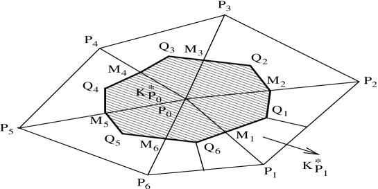
Figure 1: The control Volumes for the boundary nodes

We consider a FV element discretization of (1) in the standard $C^{0}$-conforming piecewise linear finite element space $V_{h}$ on the primary mesh $\mathcal{T}_{h}$, which is defined by

$$V_{h}=\{v_{h}\in C^{0}(\overline{\Omega})\;:\;v_{h}|_{K}\;\mbox{is linear for all}~{}K\in\mathcal{T}_{h}\;\mbox{and}\;v_{h}|_{\partial\Omega}=0\},$$

and the dual volume element space $V_{h}^{*}$ on the dual mesh $\mathcal{T}^{*}_{h}$ given by

$$V_{h}^{*}=\{v_{h}\in L^{2}(\Omega)\;:\;v_{h}|_{K_{P_{0}}^{*}}\;\mbox{is constant for all}\;K_{P_{0}}^{*}\in\mathcal{T}_{h}^{*}\;\mbox{and}\;v_{h}|_{\partial\Omega}=0\}.$$

The semi-discrete FV element formulation for (1) is to seek $u_{h}:(0,T]\longrightarrow V_{h}$ such that

$$(u_{h}^{\prime},v_{h})+A_{h}(\mathcal{B}^{\alpha}u_{h},v_{h})=(f,v_{h})\quad\forall v_{h}\in V_{h}^{*}~{}~{}~{}~{}~{}~{}~{}~{}~{}~{}~{}~{}~{}~{}~{}~{}~{}~{}~{}~{}~{}$$ (1)

with given $u_{h}(0)\in V_{h}$ to be defined later. Here, $A_{h}(\cdot,\cdot)$ is defined by

$$A_{h}(w_{h},v_{h})=-\sum_{P_{i}\in N_{h}^{0}}v_{h}(P_{i})\int_{\partial K_{P_{i}}^{*}}\nabla w_{h}\cdot{\bf n}\,ds\quad\forall~{}w_{h}\in V_{h}~{}{\rm and}~{}v_{h}\in V_{h}^{*}\,,$$ (2)

with ${\bf n}$ denoting the outward unit normal to the boundary of the control volume $K_{P_{i}}^{*}$. For $v\in H^{2}(\Omega)$, a use of Green’s formula yields

$$(\mathcal{L}v,v_{h})=A_{h}(v,v_{h}),\quad\forall~{}v_{h}\in V_{h}^{*}\,.$$ (3)

Moreover as $\mathcal{L}=-\Delta,$ the following identity holds:

$$A(w_{h},\chi)=A_{h}(w_{h},\Pi_{h}^{\ast}\chi)\qquad\forall w_{h},\;\chi\in V_{h}.$$ (4)

Hence, taking the $L^{2}$-inner product of (1) with $v_{h}\in V_{h}^{*}$ yields

$$(u^{\prime},v_{h})+A_{h}(\mathcal{B}^{\alpha}u,v_{h})=(f,v_{h})\quad\forall~{}v_{h}\in V_{h}^{*}.$$ (5)

For the error analysis, we first introduce two interpolation operators. Let $\Pi_{h}:C^{0}(\bar{\Omega})\longrightarrow V_{h}$ be the piecewise linear interpolation operator and $\Pi_{h}^{*}:C^{0}(\bar{\Omega})\longrightarrow V_{h}^{*}$ be the piecewise constant interpolation operator. These interpolation operators are defined, respectively, by

$$\Pi_{h}u=\sum_{P_{i}\in N_{h}^{0}}u(P_{i})\phi_{i}(x)\;~{}\mbox{and}~{}\;\Pi_{h}^{*}u=\sum_{P_{i}\in N_{h}^{0}}u(P_{i})\chi_{i}(x).$$ (6)

It is known that $\Pi_{h}$ has the following approximation property (Ciarlet (1978)):

$$\|\psi-\Pi_{h}\psi\|_{0}\leq Ch^{2}\|\psi\|_{2}\quad{\rm for}\quad\psi\in H^{2}(\Omega)\,.$$ (7)

We state next the properties of the interpolation operator $\Pi_{h}^{*}.$ For a proof, see (pp. 192, Li et al. (2000)). For convenience, we introduce the following notations: $\langle\phi,v\rangle:=(\phi,\Pi_{h}^{*}v)$ for $\phi\in L^{2}$ and $v\in C^{0}(\bar{\Omega})$.

Lemma 3.1.

The following statements hold true.

• $\langle\cdot,\cdot\rangle$ defines an inner-product on $V_{h}\times V_{h}$ with its induced norm denoted by $|\|\cdot|\|.$

• The norms $|\|\cdot|\|$ and $\|\cdot\|$ are equivalent on $V_{h}$ .

• The operator $\Pi^{*}_{h}$ is stable in the following sense: $\|\Pi_{h}^{*}\chi\|\leq C\|\chi\|$ for any $\chi\in V_{h}.$

4 A Priori Error Estimates

This section deals with a priori optimal order error estimates for the semi-discrete FV scheme (1). To do so, we split the error as:

$$u_{h}-u=(u_{h}-\bar{R}_{h}u)+(\bar{R}_{h}u-u)=:\theta+\xi,$$

where $\bar{R}_{h}:H_{0}^{1}(\Omega)\cap H^{2}(\Omega)\rightarrow V_{h}$ is the finite volume elliptic projection operator defined by

$$A_{h}(\bar{R}_{h}v,\chi)=A_{h}(v,\chi)\qquad\forall\,\chi\in V_{h}^{*}.$$ (1)

For each $t\in(0,T]$, the projection error $\xi(t)$ satisfies the following estimates (Chou & Li (2000)):

$$\|\xi(t)\|_{\ell}+\|\xi^{\prime}(t)\|_{\ell}\leq Ch^{2-\ell}\Big{(}\|u(t)\|_{W^{3}_{p}}+\|u^{\prime}(t)\|_{W^{3}_{p}}\Big{)}\quad{\rm for}~{}\ell=0,1\quad{\rm with}~{}~{}p>1.$$ (2)

Moreover, the following maximum estimate is also valid for $t\in(0,T]$

$$\|\xi(t)\|_{\infty}\leq Ch^{2}|\log\left(h\right)|\Big{(}\|u(t)\|_{3}+\|u(t)\|_{W^{2,\infty}(\Omega)}\Big{)}.$$ (3)

From (1) and (5), it follows that

$$\langle\theta^{\prime},\chi\rangle+A_{h}(\mathcal{B}^{\alpha}\theta,\Pi_{h}^{*}\chi)=-(\xi^{\prime},\Pi_{h}^{*}\chi)\quad\forall~{}\chi\in V_{h}.$$ (4)

On substitution of (4) in (4), we obtain

$$\langle\theta^{\prime},\chi\rangle+A(\mathcal{B}^{\alpha}\theta,\chi)=-(\xi^{\prime},\Pi_{h}^{*}\chi)\quad\forall~{}\chi\in V_{h}\,.$$ (5)

Below, we prove one of the main theorems of this section. We may choose $u_{h}(0)=\Pi_{h}u_{0},$ or even $L^{2}$-projection onto $V_{h},$ then, using approximation property and the equivalence of norms (ii) of Lemma 3.1, it follows that $\||\theta(0)\||\leq C\|\theta(0)\|\leq Ch^{2}\;\|u_{0}\|_{2}.$ In case, we choose $u_{h}(0)=\bar{R}_{h}u_{0},$ then $\theta(0)=0.$

Theorem 4.1.

Let $u$ and $u_{h}$ be the solutions of $(\ref{eq: fractional diffusion})$ and $(\ref{semi}),$ respectively. Further, let $u_{h}(0)$ be chosen so that $\|u_{0}-u_{h}(0)\|=O(h^{2}).$ Then for any $T>0$, there is a positive constant $C,$ which may depend on $T$ and $\alpha,$ but independent of $h$ such that

$$\|(u_{h}-u)(T)\|\leq C\,h^{2}\left(\|u_{0}\|_{3}+\|u^{\prime}\|_{L^{1}(H^{3})}\right).$$

Proof 4.2.

Since $u_{h}-u=\xi+\theta,$ where the estimate of $\xi$ is given in (2), it is sufficient to estimate $\theta.$ To this end, choose $\chi=\theta$ in (5) and obtain

$$\langle\theta^{\prime},\theta\rangle+A(\mathcal{B}^{\alpha}\theta,\theta)=-(\xi^{\prime},\Pi_{h}^{*}\theta).$$ (6)

Integrating from $0$ to $t$ and using $\langle\theta^{\prime},\theta\rangle=\frac{1}{2}\frac{d}{dt}|\|\theta|\|^{2}$ yield

$$\||\theta(t)\||^{2}+2\int_{0}^{t}A(\mathcal{B}^{\alpha}\theta,\theta)\,ds\leq|\|\theta(0)|\|^{2}+2\int_{0}^{t}|(\xi^{\prime},\Pi_{h}^{*}\theta)(s)|\,ds\,.$$ (7)

By the stability property for the operator $\Pi_{h}^{*}$ in Lemma 3.1 (iii), and the equivalence of norms in Lemma 3.1 (ii), we have $|(\xi^{\prime},\Pi_{h}^{*}\theta)|\leq\,\|\xi^{\prime}\|\;\|\Pi_{h}^{*}\theta\|\leq C\|\xi^{\prime}\|\;\||\theta\||.$ On substitution this in (7), and use the positivity property of $\mathcal{B}^{\alpha}$ in (3) to obtain after simplification

$$\||\theta(t)\||^{2}\leq\||\theta(0)\||^{2}+C\,\int_{0}^{t}\|\xi^{\prime}(s)\|\;\||\theta(s)\||\;ds.$$ (8)

Let $t^{*}\in[0,t]$ be such that $\||\theta(t^{*})\||:=\max_{0\leq s\leq t}\,\||\theta(s)\||.$ Then, it is easy to check from (8) that

$$\||\theta(t)\||\leq\||\theta(t^{*})\||\leq\||\theta(0)\||+C\,\int_{0}^{t}\|\xi^{\prime}(s)\|\;ds\,.$$ (9)

Therefore, the desired error estimate follows from the decomposition $u_{h}-u=\xi+\theta$, the inequality $\|\theta(T)\|\leq C\,|\|\theta(T)|\|$ by Lemma 3.1 (ii), the above bound, the finite volume elliptic projection error (2), and the inequality $\|u(T)\|_{3}\leq\|u_{0}\|_{3}+\int_{0}^{T}\|u^{\prime}(t)\|_{3}\,dt.$ This completes the rest of the proof.

Due to the singular behaviour of the solution $u$ of (1) near $t=0$, some regularity and compatibility assumptions on the given data $u_{0}$ and $f$ are required to make sure that the term $\|u_{0}\|_{3}+\|u^{\prime}\|_{L^{1}(H^{3})}$ is bounded. Consequently, by Theorem 4.1, the error for the spatial discretization by FV method is of order $O(h^{2})$. For instance, if $f\equiv 0$, we assume that $u_{0}\in H^{4}(\Omega)\cap H^{1}_{0}(\Omega)$ and $\mathcal{L}u_{0}\in H^{1}_{0}(\Omega)$, then by (Theorem 4.2, Mclean (2010)),

$$\|u^{\prime}(t)\|_{2}+t^{\frac{\alpha}{2}}\|u^{\prime}(t)\|_{3}\leq C_{1}\,t^{\alpha-1}\quad{\rm for}~{}~{}t>0\,.$$ (10)

Hence, from Theorem 4.1, $\|(u_{h}-u)(t)\|\leq C\,h^{2}$ for $t>0.$ Here, we can argue that the assumptions on $u_{0}$ can be slightly relaxed. Instead, we assume that $u_{0}\in H^{3}(\Omega)\cap H^{1}_{0}(\Omega)$ and $\mathcal{L}u_{0}\in H^{1}_{0}(\Omega)$, and again by (Theorem 4.2, Mclean (2010)), we arrive at

$$\|u^{\prime}(t)\|_{1}+t^{\frac{\alpha}{2}}\|u^{\prime}(t)\|_{2}+t^{\alpha}\|u^{\prime}(t)\|_{3}\leq C\,t^{\alpha-1}\quad{\rm for}~{}~{}t>0\,.$$ (11)

Using the elliptic projection bound $\|\xi^{\prime}(t)\|\leq Ch\|u^{\prime}(t)\|_{2},$ and also the projection bound in (2), we observe for $\epsilon>0$ that

$$\|\xi(t)\| \leq\|\xi(0)\|+\int_{0}^{t}\|\xi^{\prime}(s)\|\,ds$$

$$\leq C\,h^{2}\left(\|u_{0}\|_{3}+h^{-1}\int_{0}^{\epsilon}\|u^{\prime}(s)\|_{2}\,ds+\int_{\epsilon}^{t}\|u^{\prime}(s)\|_{3}\,ds\right)\quad{\rm for}~{}~{}t>0.$$

Thus, by the regularity property (11), it follows that

$$\|\xi(t)\| \leq C\,h^{2}\left(\|u_{0}\|_{3}+h^{-1}\int_{0}^{\epsilon}s^{\frac{\alpha}{2}-1}\,ds+\int_{\epsilon}^{t}s^{-1}\,ds\right)$$ (12)

$$\leq C\,h^{2}\left(1+h^{-1}\epsilon^{\frac{\alpha}{2}}+|{\rm log}(t/\epsilon)|\right)$$

$$\leq C\,h^{2}\left(1+|{\rm log}\;h|\right)\quad{\rm with}~{}~{}\epsilon={\min\{h^{\frac{2}{\alpha}},t\}}\,.$$

Therefore, a use of the obtained estimate of $\xi(t)$ in the proof of the Theorem 4.1 yields

$$\|(u_{h}-u)(t)\|\leq C\,h^{2}\left(1+|{\rm log}\;h|\right).$$

Our next aim is to derive an estimate of order $O(h^{2}),$ but in the stronger $L^{\infty}(L^{\infty})$-norm. To do so, we start by estimating $\theta^{\prime}$ in the next lemma. This bound is needed for showing the super-convergence result of $\nabla\theta$ in $L^{\infty}(L^{2})$-norm.

Lemma 4.3.

With $u_{h}(0)=\bar{R}_{h}u_{0},$ there exists a positive constant $C$ independent of $h$ such that

$$\int_{0}^{t}\|\theta^{\prime}\|^{2}\,ds\leq C\int_{0}^{t}\|\xi^{\prime}\|^{2}ds\quad{\rm for}~{}~{}0<t\leq T\,.$$

Proof 4.4.

Choose $\chi=\theta^{\prime}$ in (5) to obtain

$$|\|\theta^{\prime}|\|^{2}+A(\mathcal{B}^{\alpha}\theta,\theta^{\prime})=-(\xi^{\prime},\Pi_{h}^{*}\theta^{\prime}).$$

Since $\theta(0)=0$, $\mathcal{B}^{\alpha}\theta=\mathcal{I}^{\alpha}\theta^{\prime}.$ Using this and the positivity property of $\mathcal{I}^{\alpha}$, (2), we arrive at

$$\int_{0}^{t}A(\mathcal{B}^{\alpha}\theta,\theta^{\prime})\,ds=\int_{0}^{t}(\mathcal{I}^{\alpha}(\nabla\theta^{\prime}),\nabla\theta^{\prime})\,ds\geq 0\,.$$

Hence, by the Cauchy-Schwarz inequality, the stability property of $\Pi_{h}^{*}$, and also by Lemma 3.1 $(ii)$,

$$\int_{0}^{t}|\|\theta^{\prime}|\|^{2}\,ds\leq\int_{0}^{t}|(\xi^{\prime},\Pi_{h}^{*}\theta^{\prime})|\,ds\leq C\int_{0}^{t}\|\xi^{\prime}\|\,\|\theta^{\prime}\|\;ds\leq C\int_{0}^{t}\|\xi^{\prime}\|\,\||\theta^{\prime}|\|\;ds.$$

Therefore, a use of Holder’s inequality and again Lemma 3.1 $(ii)$ complete the rest of the proof.

Below, we derive an upper bound of $\nabla\theta$ in $L^{\infty}(L^{2})$-norm.

Lemma 4.5.

Assume that the solution $u$ of (1) satisfies the regularity property (10). With $u_{h}(0)=\bar{R}_{h}u_{0},$ there exists a positive constant $C,$ independent of $h,$ such that

$$\|\nabla\theta(t)\|^{2}\leq Ch^{2}\int_{0}^{t}\|\theta^{\prime}\|\,ds+Ch^{4}|\log(t/{\min\{h^{\frac{2}{\alpha}},t\}})|.$$

Proof 4.6.

Choose $\chi=\mathcal{I}^{1-\alpha}_{ad}\,\theta^{\prime}$ in (5) and integrate the resulting equation over the interval $(0,t)$. Use (5) to arrive at

$$\int_{0}^{t}\langle\mathcal{I}^{1-\alpha}\theta^{\prime},\theta^{\prime}\rangle\,ds+\int_{0}^{t}A(\theta,\theta^{\prime})\,ds=-\int_{0}^{t}(\xi^{\prime},\Pi_{h}^{*}\mathcal{I}^{1-\alpha}_{ad}\,\theta^{\prime})\,ds.$$ (13)

To bound the term on the right hand side of (13), we decompose $\xi$ as

$$\xi=(\Pi_{h}u-u)+(\bar{R}_{h}u-\Pi_{h}u)=:\xi_{1}+\xi_{2}.$$

Since $\xi_{2}\in V_{h}$ and since $\Pi_{h}^{*}$ commutes with $\mathcal{I}^{1-\alpha}_{ad}\,$,

$$\int_{0}^{t}(\xi^{\prime},\Pi_{h}^{*}\mathcal{I}^{1-\alpha}_{ad}\,\theta^{\prime})\,ds=\int_{0}^{t}(\mathcal{I}^{1-\alpha}\xi_{1}^{\prime},\Pi_{h}^{*}\theta^{\prime})\,ds+\int_{0}^{t}\langle\mathcal{I}^{1-\alpha}\xi_{2}^{\prime},\theta^{\prime}\rangle\,ds$$

By the continuity property (see Lemma 3.1(iii) in Mustapha & Schötzau (2014)) of $\mathcal{I}^{1-\alpha}$,

$$\Big{|}\int_{0}^{t}\langle\mathcal{I}^{1-\alpha}\xi_{2}^{\prime},\theta^{\prime}\rangle\,ds\Big{|}\leq C_{\alpha}\int_{0}^{t}\langle\mathcal{I}^{1-\alpha}\xi_{2}^{\prime},\xi_{2}^{\prime}\rangle\,ds+\frac{1}{2}\int_{0}^{t}\langle\mathcal{I}^{1-\alpha}\theta^{\prime},\theta^{\prime}\rangle\,ds\,.$$

Substitute the above equations in (13) and use the equality $\int_{0}^{t}A(\theta,\theta^{\prime})\,ds=\frac{1}{2}\|\nabla\theta(t)\|^{2}$ (because $\theta(0)=0$) to obtain after simplifying

$$\int_{0}^{t}\langle\mathcal{I}^{1-\alpha}\theta^{\prime},\theta^{\prime}\rangle\,ds+\|\nabla\theta(t)\|^{2}\leq 2\Big{|}\int_{0}^{t}(\mathcal{I}^{1-\alpha}\xi_{1}^{\prime},\Pi_{h}^{*}\theta^{\prime})\,ds\Big{|}+C_{\alpha}\int_{0}^{t}\langle\mathcal{I}^{1-\alpha}\xi_{2}^{\prime},\xi_{2}^{\prime}\rangle\,ds\,.$$ (14)

By the stability of $\Pi_{h}^{*},$ it follows that

$$2\Big{|}\int_{0}^{t}(\mathcal{I}^{1-\alpha}\xi_{1}^{\prime}, \Pi_{h}^{*}\theta^{\prime})\,ds\Big{|}+C_{\alpha}\int_{0}^{t}\langle\mathcal{I}^{1-\alpha}\xi_{2}^{\prime},\xi_{2}^{\prime}\rangle\,ds$$

$$\leq C\int_{0}^{t}\|\mathcal{I}^{1-\alpha}\xi_{1}^{\prime}\|\,\|\theta^{\prime}\|\,ds+C_{\alpha}\int_{0}^{t}\|\mathcal{I}^{1-\alpha}\xi_{2}^{\prime}\|\,\|\xi_{2}^{\prime}\|\,ds$$

$$\leq C\int_{0}^{t}\int_{0}^{s}(s-\tau)^{-\alpha}\Big{(}\|\xi_{1}^{\prime}(\tau)\|\,\|\theta^{\prime}(s)\|+\|\xi_{2}^{\prime}(\tau)\|\,\|\xi_{2}^{\prime}(s)\|\Big{)}\,d\tau\,ds.$$

Now split $\xi_{2}$ as $\xi_{2}=\xi-\xi_{1}$ and use the elliptic projection with (2) and (7) to arrive at

$$2\Big{|}\int_{0}^{t}(\mathcal{I}^{1-\alpha}\xi_{1}^{\prime},\Pi_{h}^{*}\theta^{\prime})\,ds\Big{|}+C\int_{0}^{t}\langle\mathcal{I}^{1-\alpha}\xi_{2}^{\prime},\xi_{2}^{\prime}\rangle\,ds$$ (15)

$$\leq Ch^{2}\int_{0}^{t}\int_{0}^{s}(s-\tau)^{-\alpha}\|u^{\prime}(\tau)\|_{2}\,\|\theta^{\prime}(s)\|\,d\tau\,ds$$

$$+Ch^{3}\Big{(}\int_{0}^{\epsilon}\|u^{\prime}(s)\|_{2}+h\int_{\epsilon}^{t}\|u^{\prime}(s)\|_{3}\Big{)}\int_{0}^{s}(s-\tau)^{-\alpha}\|u^{\prime}(\tau)\|_{3}\,\,d\tau\,ds$$

$$\leq Ch^{2}\int_{0}^{t}\|\theta^{\prime}(s)\|\,ds+Ch^{4}\Big{(}h^{-1}\int_{0}^{\epsilon}s^{\frac{\alpha}{2}-1}\,ds+\int_{\epsilon}^{t}s^{-1}\,ds\Big{)}$$

$$\leq Ch^{2}\int_{0}^{t}\|\theta^{\prime}(s)\|\,ds+Ch^{4}\;\Big{(}h^{-1}\;\epsilon^{\frac{\alpha}{2}}+\log\Big{(}\frac{t}{\epsilon}\Big{)}\Big{)}\,.$$

where in the second last step, we have used the regularity assumption (10) and the inequalities:

$$\int_{0}^{s}(s-\tau)^{-\alpha}\tau^{\frac{\alpha}{2}-1}\,d\tau\leq C\,s^{-\frac{\alpha}{2}}\quad{\rm and}\quad\int_{0}^{s}(s-\tau)^{-\alpha}\tau^{\alpha-1}\,d\tau\leq C\,.$$

Substitute (15) in (14), choose $\epsilon={\min\{h^{\frac{2}{\alpha}},t\}}$, and use the positivity property (2) of the operator $\mathcal{I}^{1-\alpha}$ to complete the rest of the proof.

As a consequence of the super-convergent result proved in Lemma 4.5, we prove in the next theorem, the following maximum norm convergence.

Theorem 4.7.

Let $u_{h}(0)=\bar{R}_{h}u_{0}.$ Assume that $u\in H^{1}(0,T;H^{3}(\Omega))\cap L^{\infty}(0,T;W^{2,\infty}(\Omega))$. Then,

$$\|(u_{h}-u)(t)\|_{\infty}\leq Ch^{2}|{\rm log}\;h\;|\quad{\rm for}~{}~{}t\in(0,T],$$

where the constant $C$ depends on $T$ and $\alpha$, but independent of $h$ .

Proof 4.8.

From the decomposition $u_{h}-u=\xi+\theta$ and the estimates of $\xi$ in (3), we obtain for $t>0$

$$\|(u_{h}-u)(t)\|_{\infty}\leq Ch^{2}\;|{\rm log}\;h\;|\;\Big{(}\|u(t)\|_{3}+\|u(t)\|_{W^{2,\infty}(\Omega)}\Big{)}+\|\theta(t)\|_{\infty}\,.$$

However, by Sobolev lemma when $\Omega\subset\mathbb{R}^{2}$ and Lemma 4.5, we arrive for $t>0$ at

$$\|\theta(t)\|_{\infty} \leq C\;|{\rm log}\;h\;|\;\|\nabla\theta(t)\|\leq Ch\;|{\rm log}\;h\;|\;\int_{0}^{t}\|\theta^{\prime}\|\,ds+Ch^{2}\;|{\rm log}\;(t/{\min\{h^{\frac{2}{\alpha}},t\}})|\,.$$

To complete the proof, we use the inequality $\int_{0}^{t}\|\theta^{\prime}\|\,ds\leq t^{1/2}\Big{(}\int_{0}^{t}\|\theta^{\prime}\|^{2}\,ds\Big{)}^{1/2}$, Lemma 4.3, the bound in (2), and the regularity assumption $u\in H^{1}(0,T;H^{3}(\Omega))$.

Remark 4.9.

The assumption $u\in H^{1}(0,T;H^{3}(\Omega))$ is stronger than the one imposed in (10). Noting that, under the regularity assumptions in (10) with $\alpha\in(1/2,1)$, one can show that the error in the $L^{\infty}(L^{\infty})$ is of order $h^{\frac{3}{2}}$ (ignoring the logarithmic factor), that is, suboptimal. To see this, we follow the derivation in the above theorem, and use

$$\int_{0}^{t}\|\theta^{\prime}\|^{2}\,ds\leq C\,\int_{0}^{t}\|\xi^{\prime}\|^{2}\,ds\leq C\,h^{2}\int_{0}^{t}\|u^{\prime}\|_{2}^{2}\,ds\leq C\,h^{2}\int_{0}^{t}s^{2\alpha-2}\,ds\leq C\,h^{2}.$$

However, our numerical experiments illustrate that the imposed regularity assumptions are pessimistic. We observe optimal rates of convergence in the absence of the regularity assumptions (10).

5 The fully-discrete numerical scheme

This section is devoted to our fully-discrete scheme for the fractional diffusion model problem (1). We discretize in time using a piecewise linear DG method (Mustapha & McLean (2011)) and the FV method for the spatial discretization. To this end, we introduce a (possibly non-uniform) partition of the time interval $[0,T]$ given by the points: $0=t_{0}<t_{1}<t_{2}<\cdots<t_{N}=T,$ and define the half-open subinterval $I_{n}=(t_{n-1},t_{n}]$ with length $k_{n}=t_{n}-t_{n-1}$ for $1\leq n\leq N$ and set  $k:=\max_{1\leq n\leq N}k_{n}$.

Next, we introduce our time-space finite dimensional spaces ${\mathcal{W}}$ and ${\mathcal{W}}^{*}$ as

$${\mathcal{W}} :=\{v\in L_{2}((0,T);V_{h}):v|_{I_{n}}\in P_{1}(V_{h}),1\leq n\leq N\},$$

$${\mathcal{W}}^{*} :=\{v\in L_{2}((0,T);V_{h}^{*}):v|_{I_{n}}\in P_{1}(V_{h}^{*}),1\leq n\leq N\},$$

where $P_{1}(S)$ denotes the space of linear polynomials in $t$ with coefficients in a given space $S.$

The DG FV approximation $U\in{\mathcal{W}}$ for (1) is now defined as follows: Given $U(t)$ for $0\leq t\leq t_{n-1}$ with $U(0):=U^{0}=U^{0}_{+}\approx u_{0}$, the solution $U\in P_{1}(V_{h})$ on $I_{n}$ is determined by requiring that for $1\leq n\leq N$,

$$(U^{n-1}_{+},X^{n-1}_{+})+\int_{I_{n}}\bigl{\{}(U^{\prime},X)+A_{h}\bigl{(}\mathcal{B}^{\alpha}U,X\bigr{)}\bigr{\}}\,dt=(U^{n-1},X^{n-1}_{+})+\int_{I_{n}}(f,X)\,dt\quad\forall~{}X\in P_{1}(V_{h}^{*}),$$ (1)

where

$$U^{n}:=U(t_{n})=U(t_{n}^{-}),\quad U^{n}_{+}:=U(t_{n}^{+}),\quad[U]^{n}:=U^{n}_{+}-U^{n}\,.$$

For our error analysis, we recast the DG FV method using the global bilinear form:

$$G(v,w):=\langle v^{0}_{+},w^{0}_{+}\rangle+\sum_{j=1}^{N-1}\langle[v]^{j},w^{j}_{+}\rangle+\sum_{j=1}^{N}\int_{I_{j}}\,\langle v^{\prime},w\rangle\,dt.$$ (2)

Integration by parts yields an alternative expression for the bilinear form as

$$G(v,w)=\langle v^{N},w^{N}\rangle-\sum_{j=1}^{N-1}\langle v^{j},[w]^{j}\rangle-\sum_{j=1}^{N}\int_{I_{j}}\langle v,w^{\prime}\rangle\,dt\,.$$ (3)

One can see that the local DG FV scheme (1) holds if and only if $U\in{\mathcal{W}}$ satisfies

$$G(U,X)+\int_{0}^{T}A_{h}\bigl{(}\mathcal{B}^{\alpha}U,\Pi_{h}^{*}X\bigr{)}\,dt=\langle U^{0},X^{0}_{+}\rangle+\int_{0}^{T}\langle f,X\rangle\,dt\quad\forall~{}X\in{\mathcal{W}}.$$ (4)

Since the exact solution $u$ of (1) satisfies (5) and the identity $[u]^{j}=0$ for all $j$, it follows that

$$G(u,X)+\int_{0}^{T}A_{h}\bigl{(}\mathcal{B}^{\alpha}u,\Pi_{h}^{*}X\bigr{)}\,dt=\langle u_{0},X^{0}_{+}\rangle+\int_{0}^{T}\langle f,X\rangle\,dt\,.$$

Thus, the following Galerkin orthogonality property follows at once

$$G(U-u,X)+\int_{0}^{T}A_{h}\bigl{(}\mathcal{B}^{\alpha}(U-u),\Pi_{h}^{*}X\bigr{)}\,dt=\langle U^{0}-u_{0},X^{0}_{+}\rangle\quad\forall~{}X\in{\mathcal{W}}.$$ (5)

6 Error analysis of the DG FV scheme

To estimate the error from the time-space discretization, we start from the following decomposition:

$$U-u=(U-\varPi_{{k}}\bar{R}_{h}u)+(\varPi_{{k}}u-u)+\varPi_{{k}}(\bar{R}_{h}u-u)=:\psi+\eta+\varPi_{{k}}\xi,$$ (1)

where $\bar{R}_{h}$ is the finite volume elliptic projection operator defined as in (1), and $\varPi_{{k}}:C^{0}(\overline{I}_{n};L^{2}(\Omega))\to C^{0}(\overline{I}_{n};{\mathcal{P}}_{1}(L^{2}(\Omega))$ is the local (in time) $L^{2}$-projection defined for $1\leq n\leq N$ by

$$\varPi_{{k}}v(t_{n})-v(t_{n})=0~{}~{}{\rm and}~{}~{}\int_{I_{n}}(\varPi_{{k}}v-v,w)\,dt=0~{}~{}\forall~{}w\in L_{2}(\Omega).$$ (2)

The projection $\varPi_{{k}}$ satisfies the error property (Equation 25, Mustapha & McLean (2011)):

$$\|\eta\|_{I_{n}}\leq 2k_{n}\int_{I_{n}}\|u^{\prime\prime}(t)\|\,dt\;\;\;\mbox{for}\;\;1\leq n\leq N,$$ (3)

and also the following error bound property which involves the fractional derivative operator $\mathcal{B}^{\alpha}$:

$$\Big{|}\int_{0}^{T}A(\mathcal{B}^{\alpha}\eta,\Pi_{h}^{*}X)\,dt\Big{|}\leq C\,\|X\|_{J}\,{\bf E},$$ (4)

where

$${\bf E}:=k_{1}^{\alpha}\int_{I_{1}}\|Au^{\prime}\|\,dt+\sum_{n=2}^{N}k_{n}^{1+\alpha}\int_{I_{n}}\|Au^{\prime\prime}\|\,dt\,.$$ (5)

Noting that, we used in (4) the following notations

$$\|v\|_{J}:=\max_{n=1}^{N}\|v\|_{I_{n}}\quad{\rm with}\quad\|v\|_{I_{n}}:=\sup_{t\in I_{n}}\|v(t)\|\,.$$

For the proof of (4), we refer to (Lemma 2, Mustapha & McLean (2011)) in addition, to the use of the stability property of $\Pi^{*}_{h}$ in Lemma 3.1 (iii).

Next, we estimate $\psi$. In our proof, we use the following spatial discrete analogue of (3):

$$\int_{0}^{T}A_{h}\bigl{(}\mathcal{B}^{\alpha}\chi,\Pi_{h}^{*}\chi\bigr{)}\,dt=\int_{0}^{T}A\bigl{(}\mathcal{B}^{\alpha}\chi,\chi\bigr{)}\,dt\geq c_{\alpha}T^{\alpha-1}\int_{0}^{T}\|\nabla\chi(t)\|^{2}\,dt\quad\forall~{}~{}\chi\in{\mathcal{W}},$$ (6)

which follows from the identity (4) and the coercivity property in (3).

Lemma 6.1.

Given $\psi=U-\varPi_{{k}}\bar{R}_{h}u,$ the following estimate holds

$$\|\psi\|_{J}\leq C\|U^{0}-\bar{R}_{h}u_{0}\|+\int_{0}^{T}\|\xi^{\prime}(t)\|\,dt+C\,{\bf E},$$

where ${\bf E}$ is defined in (5).

Proof 6.2.

The Galerkin orthogonality property (5) along with the decomposition (1) and the identity (4) implies that

$$G(\psi,X)+\int_{0}^{T}A_{h}\bigl{(}\mathcal{B}^{\alpha}\psi,\Pi_{h}^{*}X\bigr{)}\,dt=\langle U^{0}-u_{0},X^{0}_{+}\rangle\\ -G(\varPi_{{k}}\bar{R}_{h}u-u,X)-\int_{0}^{T}A\bigl{(}\mathcal{B}^{\alpha}(\varPi_{{k}}\bar{R}_{h}u-u),X\bigr{)}\,dt\quad\forall~{}X\in{\mathcal{W}}\,.$$ (7)

Since $\int_{I_{n}}\langle\varPi_{{k}}\bar{R}_{h}u-\bar{R}_{h}u,X^{\prime}\rangle\,dt=0$ by (2), integration by parts yields

$$\int_{I_{n}}\langle\varPi_{{k}}\bar{R}_{h}u-u,X^{\prime}\rangle\,dt =\int_{I_{n}}\langle\xi,X^{\prime}\rangle\,dt=\langle\xi^{n},X^{n}\rangle-\langle\xi^{n-1},X^{n-1}_{+}\rangle-\int_{I_{n}}\langle\xi^{\prime},X\rangle\,dt\,.$$

Hence, by the alternative formulation of $G$ in (3) with $(\varPi_{{k}}\bar{R}_{h}u-u)(t_{n})=\xi^{n}$ (by the definition of $\varPi_{{k}}$),

$$G(\varPi_{{k}}\bar{R}_{h}u-u,X) =\langle\xi^{N},X^{N}\rangle-\sum_{n=1}^{N-1}\langle\xi^{n},[X]^{n}\rangle-\sum_{n=1}^{N}\int_{I_{n}}\langle\varPi_{{k}}\bar{R}_{h}u-u,X^{\prime}\rangle\,dt$$

$$=\sum_{n=1}^{N}\langle\xi^{n},X^{n}\rangle-\sum_{n=2}^{N}\langle\xi^{n-1},X^{n-1}_{+}\rangle-\sum_{n=1}^{N}\int_{I_{n}}\langle\varPi_{{k}}\bar{R}_{h}u-u,X^{\prime}\rangle\,dt$$

$$=\langle\xi^{0},X^{0}_{+}\rangle+\sum_{n=1}^{N}\int_{I_{n}}\langle\xi^{\prime},X\rangle\,dt.$$

On the other hand, by (4), the following explicit representation of $\varPi_{{k}}\bar{R}_{h}u:$

$$\varPi_{{k}}\bar{R}_{h}u(t)=\bar{R}_{h}u(t_{j})+\Big{(}\bar{R}_{h}u(t_{j})-k_{j}^{-1}\int_{t_{j-1}}^{t_{j}}\bar{R}_{h}u(s)\,ds\Big{)}\frac{2}{k_{j}}(t-t_{j})\quad{\rm for}~{}~{}t\in I_{j},$$

the definition of the projection $\bar{R}_{h}u$, and the identity (3), we notice that

$$A\bigl{(}\mathcal{B}^{\alpha}\varPi_{{k}}\bar{R}_{h}u,\Pi_{h}^{*}X\bigr{)}=A_{h}\bigl{(}\mathcal{B}^{\alpha}\varPi_{{k}}\bar{R}_{h}u,\Pi_{h}^{*}X\bigr{)}=A_{h}\bigl{(}\mathcal{B}^{\alpha}\varPi_{{k}}u,\Pi_{h}^{*}X\bigr{)}=(\mathcal{B}^{\alpha}\mathcal{L}\varPi_{{k}}u,\Pi_{h}^{*}X)\quad{\rm on}~{}~{}I_{n}\,.$$

Substitute the above contribution in (7) and use again the identity (4) to obtain

$$G(\psi,X)+\int_{0}^{T}A\bigl{(}\mathcal{B}^{\alpha}\psi,X\bigr{)}\,dt=\langle U^{0}-\bar{R}_{h}u_{0},X^{0}_{+}\rangle-\sum_{j=1}^{N}\int_{I_{j}}\bigl{(}\langle\xi^{\prime},X\rangle+(\mathcal{B}^{\alpha}\mathcal{L}\eta,\Pi_{h}^{*}X)\bigr{)}\,dt.$$

To proceed in our proof, we choose $X=\psi$, and use the positivity property of $\mathcal{B}^{\alpha}$ in (3)) to arrive at

$$G(\psi,\psi)\leq\langle U^{0}-\bar{R}_{h}u_{0},\psi^{0}_{+}\rangle-\sum_{j=1}^{N}\int_{I_{j}}\bigl{(}\langle\xi^{\prime},\psi\rangle+(\mathcal{B}^{\alpha}\mathcal{L}\eta,\Pi_{h}^{*}\psi)\bigr{)}\,dt.$$

However, by the definition of $G$ given in (2),

$$G(\psi,\psi) =|\|\psi^{0}_{+}\||^{2}+\sum_{n=1}^{N-1}\langle[\psi]^{n},\psi^{n}_{+}\rangle+\frac{1}{2}\sum_{n=1}^{N}[|\|\psi^{n}\||^{2}-|\|\psi^{n-1}_{+}\||^{2}]$$

$$=\frac{1}{2}\Big{(}\sum_{n=1}^{N-1}|\|[\psi]^{n}\||^{2}+|\|\psi^{N}\||^{2}+|\|\psi^{0}_{+}\||^{2}\Big{)}\geq\frac{1}{8}|\|\psi\||_{J}^{2},$$

where in the last step we used the fact that for $1\leq n\leq N$, $\|\psi\|_{I_{n}}=\max\{\|\psi^{n}\|,\|\psi^{n-1}_{+}\|\}$ and the following inequality $\|\psi^{n-1}_{+}\|^{2}=\|\psi^{n-1}+[\psi]^{n-1}\|^{2}\leq 2\|\psi^{n-1}\|+2\|[\psi]^{n-1}\|^{2}\,.$ Therefore,

$$|\|\psi|\|^{2}_{J}\leq C|\langle U^{0}-\bar{R}_{h}u_{0},\psi^{0}_{+}\rangle|+C\Big{|}\int_{0}^{T}\bigl{[}(\xi^{\prime},\Pi_{h}^{*}\psi)+(\mathcal{B}^{\alpha}\mathcal{L}\eta,\Pi_{h}^{*}\psi)\bigr{]}\,dt\Big{|}\,.$$

By the stability property of $\Pi_{h}^{*}$ and the equivalence of the norms $\|\cdot\|$ and $|\|\cdot\||$ on $V_{h}$, Lemma 3.1,

$$\|\psi\|^{2}_{J}\leq C\|\psi\|_{J}\Big{(}\|U^{0}-\bar{R}_{h}u_{0}\|+\int_{0}^{T}\|\xi^{\prime}\|\,dt\Big{)}+C\Big{|}\int_{0}^{T}(\mathcal{B}^{\alpha}\mathcal{L}\eta,\Pi_{h}^{*}\psi)\,dt\Big{|},$$

and finally, the desired result follows after substituting the estimate (4) in the above inequality.

In the next theorem, we prove the main convergence results of the fully-discrete scheme. Following Mustapha & McLean (2011, 2013), we employ time graded meshes based on concentrating the time-steps near $t=0$ to compensate the singular behavior of $u$ of problem (1).

To this end, for a chosen mesh grading parameter $\gamma\geq 1$, we assume that

$$t_{n}=(n/N)^{\gamma}T\quad\text{for $0\leq n\leq N$.}$$ (8)

It is clear that for $2\leq n\leq N$, this time mesh has the following properties:

$$\gamma 2^{1-\gamma}k\,{t_{n}}^{1-\frac{1}{\gamma}}\leq{k_{n}}\leq\gamma\,k\,{t_{n}}^{1-\frac{1}{\gamma}}~{}~{}{\rm and}~{}~{}t_{n}\leq 2^{\gamma}{t_{n-1}}.$$ (9)

Under suitable regularity assumptions on the solution $u$, we achieve a convergence rate of order $h^{2}+k^{1+\alpha}$ in the $L^{\infty}(L^{2})$-norm, that is, optimal in space but suboptimal in time. However, the numerical results demonstrate optimal rates of convergence in both variables, in the stronger $L^{\infty}(L^{\infty})$-norm.

Theorem 6.3.

Assume that the solution $u$ of  (1) has the regularity properties (11) in addition to following property

$$\|u^{\prime}(t)\|+t\|u^{\prime\prime}(t)\|+t^{\alpha}\|Au^{\prime}(t)\|+t^{1+\alpha}\|Au^{\prime\prime}(t)\|\leq Mt^{\sigma-1}\quad\text{for $0<t\leq T$}$$ (10)

for some $M,\,\sigma>0$. Assume that the initial data $u_{0}\in H^{1}(\Omega)$. Let $U$ be the DG FV solution defined by (1) with $U^{0}=\bar{R}_{h}u_{0}$. Then, there is a positive constant $C$, depends on $\alpha$, $T$, $M$, $\sigma$ and $\gamma$, such that

$$\|U-u\|_{J}\leq Ch^{2}\left(1+|{\rm log}\;h|\right)+Ck^{1+\alpha}\quad{\rm for}~{}~{}\gamma>(1+\alpha)/\sigma\,.$$

Proof 6.4.

Using the decomposition (1), the stability property of the time projection $\varPi_{{k}}$: $\|\varPi_{{k}}\xi\|_{J}\leq 3\|\xi\|_{J}$ (see Equation 26, Mustapha & McLean (2011)), the inequality $\|\xi\|_{J}\leq\|\xi_{0}\|+\int_{0}^{T}\|\xi^{\prime}(t)\|\,dt$, the achieved estimate of $\psi$ in Lemma 6.1, and the bound in (12), we observe that

$$\|U-u\|_{J} \leq\|\psi\|_{J}+\|\eta\|_{J}+3\|\xi\|_{J}$$

$$\leq\|\eta\|_{J}+C\Big{(}\|\xi_{0}\|+\int_{0}^{T}\|\xi^{\prime}(t)\|\,dt+{\bf E})$$

$$\leq\|\eta\|_{J}+C\,h^{2}\left(1+|{\rm log}\;h|\right)+C{\bf E},$$

where ${\bf E}$ is defined in (5). From the bound of $\eta$ in (3), the regularity assumption (10), the time mesh property (9), and the corresponding grading mesh assumption $\gamma>(1+\alpha)/\sigma$,

$$\|\eta\|_{J}\leq\int_{I_{1}}\|u^{\prime}(t)\|\,dt+C\max_{n=1}^{N}k_{n}\int_{I_{n}}\|u^{\prime\prime}(t)\|\,dt\leq C\,t_{1}^{\sigma}+C\max_{n=1}^{N}k_{n}^{2}t_{n}^{\sigma-2}\\ \leq C\,k^{\gamma\sigma}+C\max_{n=1}^{N}k_{n}^{1+\alpha}t_{n}^{\sigma-(1+\alpha)}\leq C\,k^{\gamma\sigma}+Ck^{1+\alpha}\max_{n=1}^{N}t_{n}^{\sigma-(1+\alpha)/\gamma}\leq C\,k^{1+\alpha}.$$

In a similar fashion, we estimate ${\bf E}$ as

$${\bf E} \leq C\int_{I_{1}}t^{\sigma-1}\,dt+C\sum_{j=2}^{N}k^{1+\alpha}\int_{I_{j}}t^{(1-1/\gamma)(1+\alpha)}\|Au^{\prime\prime}(t)\|\,dt$$

$$\leq Ct_{1}^{\sigma}+Ck^{1+\alpha}\sum_{j=2}^{N}\int_{I_{j}}t^{\sigma-(1+\alpha)/\gamma-1}\,dt$$

$$\leq Ck^{\gamma\sigma}+Ck^{1+\alpha}\int_{t_{1}}^{T}t^{\sigma-(1+\alpha)/\gamma-1}\,dt\leq Ck^{1+\alpha}\quad{\rm for}~{}~{}\gamma>(1+\alpha)/\sigma\,.$$

Therefore, to complete the proof, we combine the above estimates.

7 Numerical Experiments

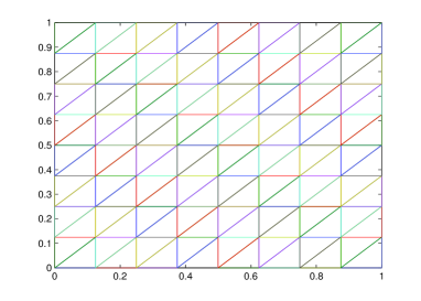
Figure 2: The FV element mesh $\mathcal{T}_{h}$ with $M=8$.

In this section, we present some numerical tests to validate our theoretical predictions from the fully-discrete DG FV scheme (4). We actually demonstrate that our achieved convergence rates are pessimistic and also the imposed regularity assumptions in our error analysis are not sharp. More precisely, for a sufficiently graded time meshes of the form (8), our tests reveal optimal convergence rates in both time and space (that is, of order $O(k^{2}+h^{2})$ in the stronger $L^{\infty}(L^{\infty})$-norm under weaker regularity conditions. However, Theorem 6.3 suggest $O(k^{\alpha+1}+h^{2})$ rates of convergence in the $L^{\infty}(L^{2})$-norm.

In our test example, we consider $\Omega=(0,1)\times(0,1)$ and $[0,T]=[0,1]$ in the fractional diffusion problem (1). We choose the initial data $u_{0}$ and the source term $f$ such that the exact solution $u(x,t)=t^{\alpha}\sin(\pi x)\sin(\pi y),$ and therefore our regularity assumptions (11) and (10) hold for $\sigma=\alpha$.

We employ time meshes of the form (8) for various choices of the mesh grading parameter $\gamma\geq 1$. Let $\mathcal{T}_{h}$ be a family of uniform (right-angle) triangular mesh of the domain $\Omega$ with diameter  $h=\sqrt{2}/M$, see Figure 2. For measuring the error in our numerical solution, we introduce a time finer grid

$$\mathcal{G}_{N,m}=\{\,t_{j-1}+qk_{j}:1\leq j\leq N,0\leq q\leq m\,\}$$

and let ${\mathcal{N}}_{h}$ be the set of all triangular nodes of the mesh family $\mathcal{T}_{h_{s}}$ where the diameter $h_{s}$ is half the diameter of the finest mesh $\mathcal{T}_{h}$ in our spatial iterations, for instance, $h_{s}=\sqrt{2}/320$ in Table 1. Define the following discrete-time-space maximum norm

$$|\|v\||_{d,m}:=\max\{|v({\bf x},t)|,~{}({\bf x},t)\in{\mathcal{N}}_{h}\times\mathcal{G}_{N,m}\}\,.$$

Thus, for large values of $N,M$ and $m$, $|\|U-u\||_{d,m}$ approximates the error measured in $L^{\infty}(L^{\infty})$.

To demonstrate the convergence rates from the spatial discretization by FV method, we refine the time steps so that the FV errors are dominant. This is achieved by fixing the ratio $\frac{k^{1+\alpha}}{h^{2}}$ to a given number $<1$. Hence, ignoring the logarithmic term, by Theorem 6.3, an error of order $O(h^{2})$ in the $L^{2}$-norm is expected. Noting here, for the semi discrete FV scheme (1), we proved in Theorem 4.7 an $O(h^{2})$ rate of convergence in the stronger $L^{\infty}(L^{\infty})$-norm under the assumption that the solution $u$ of (1) is in $H^{1}(H^{3})\cap L^{\infty}(W^{2,\infty})$. Indeed, this assumption holds for $\alpha>1/2$ in the current example. However, the numerical results in Table 1 illustrate optimal $O(h^{2})$ rates of convergence for both $\alpha<1/2$ and $\alpha>1/2.$ So, the imposed regularity assumptions may not be practically required.

To illustrate the convergence rates from time discretization by piecewise linear DG method, we refine the spatial FV meshes so that the time-stepping error dominates the spatial error. For $\alpha=0.6$, we observe from Table 2 convergence rates of order $O(k^{\min\{2,\alpha\gamma\}})$ which is optimal for $\gamma\geq 2/\alpha$. However, a suboptimal convergence of order $O(k^{1+\alpha})$ is proved in Theorem 6.3 assuming that $\gamma>(1+\alpha)/\alpha$.

$M$	$\alpha=0.4$		$\alpha=0.75$
10	3.6522e-02		3.1396e-02
20	9.6096e-03	1.9262	8.2601e-03	1.9263
40	2.4235e-03	1.9873	2.0831e-03	1.9874
80	5.8239e-04	2.0570	5.0059e-04	2.0570
120	2.4903e-04	2.0953	2.3145e-04	1.9026
160	1.3923e-04	2.0211	1.2713e-04	2.0827

Table 1: The error $|\|U-u\||_{d,10}$ and the spatial rates of convergence for different choices of $\alpha$.

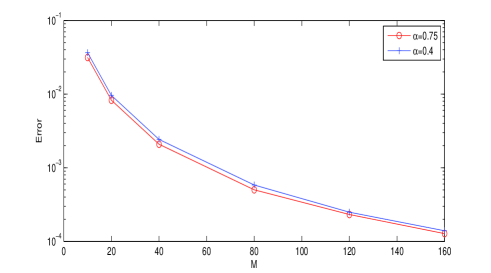
Figure 3: The FV error for $\alpha=0.4$ and $\alpha=0.75$.

$N$	$\gamma=1$		$\gamma=2$		$\gamma=3.4$
10	1.0313e-02		3.2357e-03		2.0414e-03
20	7.2124e-03	0.5159	1.5719e-03	1.0416	6.2591e-04	1.7055
40	5.0788e-03	0.5060	7.3189e-04	1.1028	1.7878e-04	1.8078
60	4.1411e-03	0.5034	4.6047e-04	1.1428	8.4038e-05	1.8619
80	3.5604e-03	0.5252	3.2953e-04	1.1630

Table 2: The error $|\|U-u\||_{d,10}$ and the temporal convergence rates for $\alpha=0.6$ with different choices of the mesh grading parameter $\gamma$.

References

- (1) E. E. Adams and L. W. Gelhar (1992), Field study of dispersion in a heterogeneous aquifer: 2. spatial moments analysis, Water Res. Research, 28, 3293-3307.
- (2) R. E. Bank, and D. J. Rose (1987), Some error estimates for the box method, SIAM J. Numer. Anal., 24, 777-787.
- (3) Z. Cai (1991), On the finite volume element method, Numer. Math., 58, 713-735.
- (4) P. Chatzipantelidis, R. D. Lazarov and V. Thomée (2004), Error estimates for a finite volume element method for parabolic equations in convex polygonal domains, Numer. Meth. PDE, 20, 650-674.
- (5) P. Chatzipantelidis, R. D. Lazarov and V. Thomée (2009), Parabolic finite volume element equation in nonconvex polygonal domains, Numer. Meth. PDE, 25, 507-525.
- (6) C.-M. Chen, F. Liu, V. Anh, I. Turner (2012), Numerical methods for solving a two-dimensional variable-order anomalous sub-diffusion equation, Math. Comput., 81, 345-366.
- (7) S. H. Chou and Q. Li (2000), Error estimates in , and in covolume methods for elliptic and parabolic problems: A unified approach, Math. Comp., 69, 103-120.
- (8) S. H. Chou, D. Y. Kwak and Q. Li (2003), error estimates and superconvergence for covolume or finite volume element methods, Numer. Meth. PDE, 19, 463-486.
- (9) P. G. Ciarlet (1978), The finite element method for elliptic problems, North Holland, Amsterdam.
- (10) B. Cockburn, and K. Mustapha (2015), A hybridizable discontinuous Galerkin method for fractional diffusion problems, Numer. Math., 130, 293–314
- (11) E. Cuesta, C. Lubich and C. Palencia (2006), Convolution quadrature time discretization of fractional diffusive-wave equations, Math. Comput., 75, 673–696.
- (12) M. R. Cui (2009), Compact finite difference method for the fractional diffusion equation, J. Comput. Phys., 228, 7792–7804.
- (13) R. E. Ewing, R. D. Lazarov, and Y. Lin (2000), Finite volume element approximations of nonlocal reactive flows in porous media, Numer. Meth. PDEs, 16, 285-311.
- (14) Y. Hatano and N. Hatano (1998), Dispersive transport of ions in column experiments: An explanation of long-tailed profiles, Water Res. Research, 34, 1027–1033.
- (15) B. I. Henry and S. L. Wearne (2000), Fractional reaction-diffusion, Physica A, 276, 448-455.
- (16) T. A. M. Langlands and B. I. Henry (2005), The accuracy and stability of an implicit solution method for the fractional diffusion equation, J. Comput. Phys., 205, 719-936.
- (17) R. H. Li, Z. Y. Chen and W. Wu (2000), Generalized Difference Methods for Differential Equations, Marcel Dekker, New York.
- (18) W. Mclean (2010), Regularity of solutions to a time-fractional diffusion equation, ANZIAM J., 52, 123-138.
- (19) W. Mclean (2012), Fast summation by interval clustering for an evolution equation with memory, SIAM J. Sci. Comput., 34, A3039-A3056.
- (20) W. McLean and K. Mustapha (2009), Convergence analysis of a discontinuous Galerkin method for a fractional diffusion equation, Numer. Algor., 52, 69-88.
- (21) W. McLean and K. Mustapha (2015), Time-stepping error bounds for fractional diffusion problems with non-smooth initial data, J. Comput. Phys., 293, 201–217.
- (22) K. Mustapha (2011), An implicit finite difference time-stepping method for a sub-diffusion equation, with spatial discretization by finite elements, IMA J. Numer. Anal., 31, 719-739.
- (23) K. Mustapha (2015), Time-stepping discontinuous Galerkin methods for fractional diffusion problems, Numer. Math., 130, 497-—516.
- (24) K. Mustapha and W. McLean (2011), Piecewise-linear, discontinuous Galerkin method for a fractional diffusion equation, Numer. Algor., 56, 159-184.
- (25) K. Mustapha and W. McLean (2013), Superconvergence of a discontinuous Galerkin method for fractional diffusion and wave equations, SIAM J. Numer. Anal., 51, 491-515.
- (26) K. Mustapha and D. Schötzau (2014), Well-posedness of version discontinuous Galerkin methods for fractional diffusion wave equations, IMA J. Numer. Anal., 34, 1226-1246.
- (27) R. R. Nigmatulin (1986), The realization of the generalized transfer equation in a medium with fractal geometry, Phys. Stat. Sol. B, 133, 425-430.
- (28) I. Podlubny (1999), Fractional Differential Equations, Academic Press, San Diego.
- (29) J. Quintana-Murillo and S. B. Yuste (2013), A finite difference method with non-uniform timesteps for fractional diffusion and diffusion-wave equations, Eur. Phys. J. Spec. Top., 222, 1987-1998.
- (30) E. Süli (1991), Convergence of finite volume schemes for Poisson equation on nonuniform meshes, SIAM J. Numer. Anal., 28, 1419-1430.
- (31) Y-N Zhang, Z-Z Sun and H-L Liao (2014), Finite difference methods for the time fractional diffusion equation on non-uniform meshes, J. Comput. Phys., 265, 195-210.