Explicit high-order non-canonical symplectic particle-in-cell algorithms for Vlasov-Maxwell systems

Abstract

Explicit high-order non-canonical symplectic particle-in-cell algorithms for classical particle-field systems governed by the Vlasov-Maxwell equations are developed. The algorithm conserves a discrete non-canonical symplectic structure derived from the Lagrangian of the particle-field system, which is naturally discrete in particles. The electromagnetic field is spatially-discretized using the method of discrete exterior calculus with high-order interpolating differential forms for a cubic grid. The resulting time-domain Lagrangian assumes a non-canonical symplectic structure. It is also gauge invariant and conserves charge. The system is then solved using a structure-preserving splitting method discovered by He et al., which produces five exactly-soluble sub-systems, and high-order structure-preserving algorithms follow by combinations. The explicit, high-order, and conservative nature of the algorithms is especially suitable for long-term simulations of particle-field systems with extremely large number of degrees of freedom on massively parallel supercomputers. The algorithms have been tested and verified by the two physics problems, i.e., the nonlinear Landau damping and the electron Bernstein wave.

I Introduction

The importance of numerical solutions for the Vlasov-Maxwell (VM) system cannot be overemphasized. In most cases, important and interesting characteristics of the VM system are the long-term behaviors and multi-scale structures, which demand long-term accuracy and fidelity of numerical calculations. Conventional algorithms for the VM systems used in general do not preserve the geometric structures of the physical systems, such as the local energy-momentum conservation law and the symplectic structure. For these algorithms, the truncation errors are small only for each time-step. For example, the truncation error of a fourth order Runge-Kutta method is of the fifth order of the step-size for each time-step. However, numerical errors from different time-steps accumulate coherently with time and long-term simulation results are not reliable. To overcome this difficult, a series of geometric algorithms, which preserve the geometric structures of theoretical models in plasma physics have been developed recently.

At the single particle level, canonical Hamilton equation for charged particle dynamics can be integrated using the standard canonical symplectic integrators developed in the late 1980s Ruth (1983); Feng (1985, 1986); Feng and Qin (2010); Forest and Ruth (1990); Channell and Scovel (1990); Candy and Rozmus (1991); Marsden and West (2001); Hairer et al. (2002). Since the Hamiltonian expressed in terms of the canonical momentum is not separable, it is believed that symplectic algorithms applicable are in general implicit. Recent studies show that this is not the case, and high order explicit symplectic algorithms for charged particle dynamics have been discovered Chin (2008); He et al. (2015a, b).

For the most-studied guiding center dynamics in magnetized plasmas, a non-canonical variational symplectic integrator has been developed and applied Qin and Guan (2008); Qin et al. (2009); Li et al. (2011); Squire et al. (2012a); Kraus (2013); Zhang et al. (2014a); Ellison et al. (2015a). It is also recently discovered that the popular Boris algorithm is actually a volume-preserving algorithm Qin et al. (2013). This revelation stimulated new research activities Zhang et al. (2014b); Ellison et al. (2015b). For example, high-order volume-preserving methods He et al. (2015c) and relativistic volume-preserving methods Zhang et al. (2015) have been worked out systematically.

For collective dynamics of the particle-field system governed by the Vlasov-Maxwell equations Qin et al. (2007, 2014), Squire et al. Squire et al. (2012b, c) constructed the first geometric, structure-preserving algorithm by discretizing a geometric variational principle Qin et al. (2007). It has been applied in simulation studies of nonlinear radio-frequency waves in magnetized plasmas Xiao et al. (2013, 2015). Similar methods apply to Vlasov-Poisson system as well Evstatiev and Shadwick (2013); Evstatiev (2014); Shadwick et al. (2014). We can also discretize directly the Poisson structures of the Vlasov-Maxwell system. A canonical symplectic Particle-in-Cell (PIC) algorithm is found by discretizing the canonical Poisson bracket Qin et al. (2015a), and non-canonical symplectic methods are being developed using the powerful Hamiltonian splitting technique Crouseilles et al. (2015); Qin et al. (2015b); He et al. (2015a) that preserve the non-canonical Morrison-Marsden-Weinstein bracket Morrison (1980); Weinstein and Morrison (1981); Marsden and Weinstein (1982); Burby et al. (2015) for the VM equations. Of course, geometric structure-preserving algorithms are expected for reduced systems as well. For example, an structure-preserving algorithm has been developed for ideal MHD equations Zhou et al. (2014), and applied to study current sheet formation in an ideal plasma without resistivity Zhou et al. (2015). The superiority of these geometric algorithms has been demonstrated. This should not be surprising because geometric algorithms are built on the more fundamental field-theoretical formalism, and are directly linked to the perfect form, i.e., the variational principle of physics. The fact that the most elegant form of theory is also the most effective algorithm is philosophically satisfactory.

In this paper, we present an explicit, high order, non-canonical symplectic PIC algorithm for the Vlasov-Maxwell system. The algorithm conserves a discrete non-canonical symplectic structure derived from the Lagrangian of the particle-field system Qin et al. (2007, 2014). The Lagrangian is naturally discrete in particles, and the electromagnetic field is discretized using the method of discrete exterior calculus (DEC). An important technique for interpolating differential forms over several grid cells are developed, which generalizes the construction of Whitney forms to higher orders. The resulting Lagrangian is continuous in time and assumes a non-canonical symplectic structure, the dimension of which is finite but large. Because the electromagnetic field is interpolated as differential forms, the time-domain Lagrangian is also gauge invariant and conserves charge. From this Lagrangian, we can readily derive the non-canonical symplectic structure for the dynamics, and the system is solved using a splitting method discovered by He et al. He et al. (2015a, b). The splitting produces five exactly-soluble sub-systems, and high-order structure-preserving algorithms follow by combinations. We note that for previous symplectic PIC methods Squire et al. (2012b, c); Xiao et al. (2013, 2015); Qin et al. (2015a), high-order algorithms are implicit in general, and only the first order method can be made explicit Qin et al. (2015a). The explicit and high-order nature of the symplectic algorithms developed in the present study made it especially suitable for long-term simulations of particle-field systems with extremely large number of degrees of freedom on massively parallel supercomputers.

The paper is organized as follows. The non-canonical symplectic PIC algorithm is derived in Sec. II with an appendix on Whitney forms and their generalization to high orders. In Sec. III, the developed algorithm is tested and verified by two physics problems, i.e., the nonlinear Landau damping and the electron Bernstein wave.

II Non-Canonical Symplectic Particle-in-Cell Algorithms

We start from the Lagrangian of a collection of charged particles and electromagnetic field Qin et al. (2007, 2014)

$$L = \iiint\mathrm{d}\mathbf{x}\left(\frac{\epsilon_{0}}{2}\left(-\dot{\mathbf{A}}\left(\mathbf{x}\right)-\nabla\phi\left(\mathbf{x}\right)\right)^{2}-\frac{1}{2\mu_{0}}\left(\nabla\times\mathbf{A}\left(\mathbf{x}\right)\right)^{2}+\right.$$ (1)

$$\left.\sum_{s}\delta\left(\mathbf{x}-\mathbf{x}_{s}\right)\left(\frac{1}{2}m_{s}\dot{\mathbf{x}}_{s}^{2}+q_{s}\mathbf{A}\left(\mathbf{x}\right)\cdot\dot{\mathbf{x}}_{s}-q_{s}\phi\left(\mathbf{x}\right)\right)\right)\leavevmode\nobreak\ ,$$

where $\mathbf{A}\left(\mathbf{x}\right)$ and $\phi\left(\mathbf{x}\right)$ are the vector and scalar potentials of the electromagnetic field, $\mathbf{x}_{s}$, $m_{s}$ and $q_{s}$ denote the location, mass and charge of the $s$-th particle, and $\epsilon_{0}$ and $\mu_{0}$ are the permittivity and permeability in vacuum. We let $\epsilon_{0}=\mu_{0}=1$ to simplify the notation.

This Lagrangian is naturally discrete in particles, and we choose to discretize the electromagnetic field in a cubic mesh. To preserve the symplectic structure of the system, the method of Discrete Exterior Calculus (DEC) Hirani (2003) is used. The DEC theory in cubic meshes can be found in Ref. Stern et al. (2015). For field-particle interaction, the interpolation function is used to obtain continuous fields from discrete fields. The spatially-discretized Lagrangian $L_{sd}$ can be written as follows

$$L_{sd}=\frac{1}{2}\left(\sum_{J}\left(-\dot{\mathbf{A}}_{J}-\sum_{I}{\nabla_{\mathrm{d}}}_{JI}\phi_{I}\right)^{2}-\sum_{K}\left(\sum_{J}{\mathrm{curl_{d}}}_{KJ}\mathbf{A}_{J}\right)^{2}\right)\Delta V+\\ \sum_{s}\left(\frac{1}{2}m_{s}\dot{\mathbf{x}}_{s}^{2}+q_{s}\left(\dot{\mathbf{x}}_{s}\cdot\sum_{J}W_{\sigma_{1J}}\left(\mathbf{x}_{s}\right)\mathbf{A}_{J}-\sum_{I}W_{\sigma_{0I}}\left(\mathbf{x}_{s}\right)\phi_{I}\right)\right)\leavevmode\nobreak\ ,$$ (2)

where integers $I$, $J$ and $K$ are indices of grid points, and $\nabla_{\mathrm{d}}$ and ${\mathrm{curl_{d}}}$ are the discrete gradient and curl operators, which are linear operators on the discrete fields $\mathbf{A}_{J}$ and $\phi_{I}$. Functions $W_{\sigma_{0J}}$ and $W_{\sigma_{1I}}$ are interpolation functions for 0-forms (e.g. scalar potential) and 1-forms (e.g. vector potential), respectively. They should be viewed as maps operating on the discrete 1-form $\mathbf{A}_{J}$ and 0-form $\phi_{I}$ to generate continuous forms. More precisely, $W_{\sigma_{1J}}\left(\mathbf{x}_{s}\right)\mathbf{A}_{J}$ are the components of the continuous 1-form interpolated from the discrete 1-form $\mathbf{A}_{J}$. The idea of form interpolation maps is due to Whitney, and interpolated forms are called Whitney forms. The original Whitney forms Whitney (1957) are first order and only for forms in simplicial meshes (e.g. triangle and tetrahedron meshes). In the present study, we have developed high-order interpolation maps for a cubic mesh. The details of the construction of $\nabla_{\mathrm{d}}$, ${\mathrm{curl_{d}}}$, $W_{\sigma_{0I}}$, $W_{\sigma_{1J}}$ , and the interpolating function for 2-forms (e.g. magnetic fields) $W_{\sigma_{2K}}$ are presented in Appendix A. The major new feature of the form interpolation method adopted here is that the interpolation for electric field and magnetic field are different. Even for components in different directions of the same field, the interpolation functions are not the same. This is very different from traditional cubic interpolations used in conventional PIC methods Birdsall and Langdon (1991); Hockney and Eastwood (1988); Nieter and Cary (2004), where the same interpolation function is used for all components of electromagnetic fields. The advanced form interpolation method developed in the present study guarantees the geometric properties of the continuous system are preserved by the discretized system.

The action integral is

$$S=\int\mathrm{d}tL_{sd}\leavevmode\nobreak\ ,$$ (3)

and the dynamic equations are obtained from Hamilton’s principle,

$$\frac{\delta S}{\delta\mathbf{A}_{J}} = 0\leavevmode\nobreak\ ,$$ (4)

$$\frac{\delta S}{\delta\phi_{I}} = 0\leavevmode\nobreak\ ,$$ (5)

$$\frac{\delta S}{\delta\mathbf{x}_{s}} = 0\leavevmode\nobreak\ .$$ (6)

Equations (4) and (5) are Maxwell’s equations, and Eq. (6) is Newton’s equation with the Lorentz force for the $s$-th particle. For the dynamics to be gauge independent Squire et al. (2012a), it requires that the discrete differential operators and interpolation functions satisfy the following relations,

$$\nabla\sum_{I}W_{\sigma_{0I}}\left(\mathbf{x}\right)\phi_{I}=\sum_{I,J}W_{\sigma_{1J}}\left(\mathbf{x}\right){\nabla_{\mathrm{d}}}_{JI}\phi_{I}\leavevmode\nobreak\ ,$$ (7)

$$\nabla\times\sum_{J}W_{\sigma_{1J}}\left(\mathbf{x}\right)\mathbf{A}_{J}=\sum_{J,K}W_{\sigma_{2K}}\left(\mathbf{x}\right){{\mathrm{curl_{d}}}}_{KJ}\mathbf{A}_{J}\leavevmode\nobreak\ .$$ (8)

The gauge independence of this spatially-discretized system implies that the dynamics conserves charge automatically.

Since the dynamics are gauge independent, we can choose any gauge that is convenient. For simplicity, the temporal gauge, i.e. $\phi_{I}=0$, is adopted in the present study. To obtain the non-canonical symplectic structure and Poisson bracket, we look at the Lagrangian 1-form $\gamma$ for the spatially-discretized system defined by $S=\int\gamma$ . Let $q=[\mathbf{A}_{J},\mathbf{x}_{s}]$, and the Lagrangian 1-form can be written as

$$\gamma=\frac{\partial L_{sd}}{\partial\dot{q}}\mathbf{d}q-H\mathbf{d}t\leavevmode\nobreak\ ,$$ (9)

where $\mathbf{d}$ denotes the exterior derivative. In Eq. (9),

$$\frac{\partial L_{sd}}{\partial\dot{q}} = [\dot{\mathbf{A}}_{J}\Delta V,m_{s}\dot{\mathbf{x}}_{s}+q_{s}\sum_{J}W_{\sigma_{1J}}\left(\mathbf{x}_{s}\right)\mathbf{A}_{J}]\leavevmode\nobreak\ ,$$ (10)

and

$$H = \frac{\partial L_{sd}}{\partial\dot{q}}\dot{q}^{T}-L_{sd}\leavevmode\nobreak\$$ (11)

$$= \frac{1}{2}\Delta V\left(\sum_{J}\dot{\mathbf{A}}_{J}^{2}+\sum_{K}\left(\sum_{J}{\mathrm{curl_{d}}}_{KJ}\mathbf{A}_{J}\right)^{2}\right)+\sum_{s}\frac{1}{2}m_{s}\dot{\mathbf{x}}_{s}^{2}\leavevmode\nobreak\$$ (12)

is the Hamiltonian. The dynamical equation of the system can be written as Qin (2005); Qin et al. (2007)

$$i_{[\dot{q},\ddot{q},1]}\mathbf{d}\gamma=0\leavevmode\nobreak\ ,$$ (13)

where $[\dot{q},\ddot{q},1]$ represent vector field $\dot{q}\frac{\partial}{\partial q}+\ddot{q}\frac{\partial}{\partial\dot{q}}+\frac{\partial}{\partial t}.$ The non-canonical symplectic structure is

$$\Omega=\mathbf{d}\left(\frac{\partial L_{sd}}{\partial\dot{q}}\mathbf{d}q\right)\leavevmode\nobreak\ ,$$ (14)

and the dynamical equation (13) is equivalent to

$$\frac{d}{dt}\left[\begin{array}[]{c}\mathbf{A}_{J}\\ \mathbf{x}_{s}\\ \dot{\mathbf{A}}_{J}\\ \dot{\mathbf{x}}_{s}\end{array}\right] = \Omega^{-1}\left[\begin{array}[]{c}\frac{\partial}{\partial\mathbf{A}_{J}}\\ \frac{\partial}{\partial\mathbf{x}_{s}}\\ \frac{\partial}{\partial\dot{\mathbf{A}}_{J}}\\ \frac{\partial}{\partial\dot{\mathbf{x}}_{s}}\end{array}\right]H\leavevmode\nobreak\ .$$ (23)

The corresponding non-canonical Poisson bracket is

$$\left\{F,G\right\}=\left[\frac{\partial F}{\partial\mathbf{A}_{J}},\frac{\partial F}{\partial\mathbf{x}_{s}},\frac{\partial F}{\partial\dot{\mathbf{A}}_{J}},\frac{\partial F}{\partial\dot{\mathbf{x}}_{s}}\right]\Omega^{-1}\left[\frac{\partial G}{\partial\mathbf{A}_{J}},\frac{\partial G}{\partial\mathbf{x}_{s}},\frac{\partial G}{\partial\dot{\mathbf{A}}_{J}},\frac{\partial G}{\partial\dot{\mathbf{x}}_{s}}\right]^{T},$$ (24)

or more specifically,

$$\left\{F,G\right\} = \frac{1}{\Delta V}\sum_{J}\left(\frac{\partial F}{\partial\mathbf{A}_{J}}\cdot\frac{\partial G}{\partial\dot{\mathbf{A}}_{J}}-\frac{\partial F}{\partial\dot{\mathbf{A}}_{J}}\cdot\frac{\partial G}{\partial\mathbf{A}_{J}}\right)+\sum_{s}\frac{1}{m_{s}}\left(\frac{\partial F}{\partial\mathbf{x}_{s}}\cdot\frac{\partial G}{\partial\dot{\mathbf{x}}_{s}}-\frac{\partial F}{\partial\dot{\mathbf{x}}_{s}}\cdot\frac{\partial G}{\partial\mathbf{x}_{s}}\right)+$$ (25)

$$\sum_{s}\frac{q_{s}}{m_{s}\Delta V}\left(\frac{\partial G}{\partial\dot{\mathbf{x}}_{s}}\cdot\sum_{J}W_{\sigma_{1J}}\left(\mathbf{x}_{s}\right)\frac{\partial F}{\partial\dot{\mathbf{A}}_{J}}-\frac{\partial F}{\partial\dot{\mathbf{x}}_{s}}\cdot\sum_{J}W_{\sigma_{1J}}\left(\mathbf{x}_{s}\right)\frac{\partial G}{\partial\dot{\mathbf{A}}_{J}}\right)+$$

$$-\sum_{s}\sum_{J}\frac{q_{s}}{m_{s}^{2}}\frac{\partial F}{\partial\dot{\mathbf{x}}_{s}}\cdot[\nabla\times W_{\sigma_{1J}}\left(\mathbf{x}_{s}\right)\mathbf{A}_{J}]\times\frac{\partial G}{\partial\dot{\mathbf{x}}_{s}}\leavevmode\nobreak\ .$$

Now, we introduce two new variables $\mathbf{E}_{J}$ and $\mathbf{B}_{K}$, which are the discrete electric field and magnetic field,

$$\mathbf{E}_{J}=-\dot{\mathbf{A}}_{J}\leavevmode\nobreak\ ,$$ (26)

$$\mathbf{B}_{K}=\sum_{J}{\mathrm{curl_{d}}}_{KJ}\mathbf{A}_{J}\leavevmode\nobreak\ .$$ (27)

In terms of $\mathbf{E}_{J}$ and $\mathbf{B}_{K}$, the partial derivatives with respect to $\mathbf{A}_{J}$ and $\dot{\mathbf{A}}_{J}$ are

$$\frac{\partial F}{\partial\mathbf{A}_{J}} = \sum_{K}\frac{\partial F}{\partial\mathbf{B}_{K}}{\mathrm{curl_{d}}}_{KJ}\leavevmode\nobreak\ ,$$ (28)

$$\frac{\partial F}{\partial\dot{\mathbf{A}}_{J}} = -\frac{\partial F}{\partial\mathbf{E}_{J}}\leavevmode\nobreak\ .$$ (29)

Note that ${\mathrm{curl_{d}}}_{KJ}$ in Eq. (28) is a matrix. Using Eq. (8), the Poisson bracket in terms of $\mathbf{E}_{J}$ and $\mathbf{B}_{K}$ can be written as

$$\left\{F,G\right\}=\frac{1}{\Delta V}\sum_{J}\left(\frac{\partial F}{\partial\mathbf{E}_{J}}\cdot\sum_{K}\frac{\partial G}{\partial\mathbf{B}_{K}}{\mathrm{curl_{d}}}_{KJ}-\sum_{K}\frac{\partial F}{\partial\mathbf{B}_{K}}{\mathrm{curl_{d}}}_{KJ}\cdot\frac{\partial G}{\partial\mathbf{E}_{J}}\right)+\\ \sum_{s}\frac{1}{m_{s}}\left(\frac{\partial F}{\partial\mathbf{x}_{s}}\cdot\frac{\partial G}{\partial\dot{\mathbf{x}}_{s}}-\frac{\partial F}{\partial\dot{\mathbf{x}}_{s}}\cdot\frac{\partial G}{\partial\mathbf{x}_{s}}\right)+\\ \sum_{s}\frac{q_{s}}{m_{s}\Delta V}\left(\frac{\partial F}{\partial\dot{\mathbf{x}}_{s}}\cdot\sum_{J}W_{\sigma_{1J}}\left(\mathbf{x}_{s}\right)\frac{\partial G}{\partial\mathbf{E}_{J}}-\frac{\partial G}{\partial\dot{\mathbf{x}}_{s}}\cdot\sum_{J}W_{\sigma_{1J}}\left(\mathbf{x}_{s}\right)\frac{\partial F}{\partial\mathbf{E}_{J}}\right)+\\ -\sum_{s}\frac{q_{s}}{m_{s}^{2}}\frac{\partial F}{\partial\dot{\mathbf{x}}_{s}}\cdot\left[\sum_{K}W_{\sigma_{2K}}\left(\mathbf{x}_{s}\right)\mathbf{B}_{K}\right]\times\frac{\partial G}{\partial\dot{\mathbf{x}}_{s}}\leavevmode\nobreak\ ,$$ (30)

and the Hamiltonian is

$$H=\frac{1}{2}\left(\Delta V\sum_{J}\mathbf{E}_{J}^{2}+\Delta V\sum_{K}\mathbf{B}_{K}^{2}+\sum_{s}m_{s}\dot{\mathbf{x}}_{s}^{2}\right)\leavevmode\nobreak\ .$$ (31)

The evolution equations is

$$\dot{F}=\{F,H\}\leavevmode\nobreak\ ,$$ (32)

where

$$F=[\mathbf{E}_{J},\mathbf{B}_{K},\mathbf{x}_{s},\dot{\mathbf{x}}_{s}]\leavevmode\nobreak\ .$$ (33)

This is a Hamiltonian system with a non-canonical symplectic structure or Poisson bracket. In general, symplectic integrators for non-canonical systems are difficult to construct. However, using the splitting method discovered by He et al. He et al. (2015a, b), we have found explicit high-order symplectic algorithms for this Hamiltonian system that preserve its non-canonical symplectic structure. We note that splitting method had been applied to the Vlasov equation previously without the context of symplectic structure Crouseilles et al. (2007). We split the Hamiltonian in Eq. (31) into five parts,

$$H=H_{E}+H_{B}+H_{x}+H_{y}+H_{z}\leavevmode\nobreak\ ,$$ (34)

$$H_{E}=\frac{1}{2}\Delta V\sum_{J}\mathbf{E}_{J}^{2}\leavevmode\nobreak\ ,$$ (35)

$$H_{B}=\frac{1}{2}\Delta V\sum_{K}\mathbf{B}_{K}^{2}\leavevmode\nobreak\ ,$$ (36)

$$H_{r}=\frac{1}{2}\sum_{s}m_{s}\dot{r}_{s}^{2},\quad\textrm{for }r\textrm{ in}\leavevmode\nobreak\ x,\leavevmode\nobreak\ y,\leavevmode\nobreak\ z\leavevmode\nobreak\ .$$ (37)

It turns out that the sub-system generated by each part can be solved exactly, and high-order symplectic algorithms follow by combination. The evolution equation for $H_{E}$ is $\dot{F}=\{F,H_{E}\}$, which can be written as

$$\dot{\mathbf{E}}_{J} = 0\leavevmode\nobreak\ ,$$ (38)

$$\dot{\mathbf{B}}_{K} = -\sum_{J}{\mathrm{curl_{d}}}_{KJ}\mathbf{E}_{J}\leavevmode\nobreak\ ,$$ (39)

$$\dot{\mathbf{x}}_{s} = 0\leavevmode\nobreak\ ,$$ (40)

$$\ddot{\mathbf{x}}_{s} = \frac{q_{s}}{m_{s}}\sum_{J}W_{\sigma_{1J}}\left(\mathbf{x}_{s}\right)\mathbf{E}_{J}\leavevmode\nobreak\ .$$ (41)

The exact solution $\Theta_{E}\left(\Delta t\right)$ for any time step $\Delta t$ is

$$\mathbf{E}_{J}\left(t+\Delta t\right) = \mathbf{E}_{J}\left(t\right)\leavevmode\nobreak\ ,$$ (42)

$$\mathbf{B}_{K}\left(t+\Delta t\right) = \mathbf{B}_{K}\left(t\right)-\Delta t\sum_{J}{\mathrm{curl_{d}}}_{KJ}\mathbf{E}_{J}(t)\leavevmode\nobreak\ ,$$ (43)

$$\mathbf{x}_{s}\left(t+\Delta t\right) = \mathbf{x}_{s}\left(t\right)\leavevmode\nobreak\ ,$$ (44)

$$\dot{\mathbf{x}}_{s}\left(t+\Delta t\right) = \dot{\mathbf{x}}_{s}\left(t\right)+\frac{q_{s}}{m_{s}}\Delta t\sum_{J}W_{\sigma_{1J}}\left(\mathbf{x}_{s}(t)\right)\mathbf{E}_{J}(t)\leavevmode\nobreak\ .$$ (45)

The evolution equation for $H_{B}$ is $\dot{F}=\{F,H_{B}\}$, or

$$\dot{\mathbf{E}}_{J} = \sum_{K}{\mathrm{curl_{d}}}_{KJ}\mathbf{B}_{K}\leavevmode\nobreak\ ,$$ (46)

$$\dot{\mathbf{B}}_{K} = 0\leavevmode\nobreak\ ,$$ (47)

$$\dot{\mathbf{x}}_{s} = 0\leavevmode\nobreak\ ,$$ (48)

$$\ddot{\mathbf{x}}_{s} = 0\leavevmode\nobreak\ ,$$ (49)

whose exact solution $\Theta_{B}\left(\Delta t\right)$ is

$$\mathbf{E}_{J}\left(t+\Delta t\right) = \mathbf{E}_{J}\left(t\right)+\Delta t\sum_{K}{\mathrm{curl_{d}}}_{KJ}\mathbf{B}_{K}(t)\leavevmode\nobreak\ ,$$ (50)

$$\mathbf{B}_{K}\left(t+\Delta t\right) = \mathbf{B}_{K}\left(t\right)\leavevmode\nobreak\ ,$$ (51)

$$\mathbf{x}_{s}\left(t+\Delta t\right) = \mathbf{x}_{s}\left(t\right)\leavevmode\nobreak\ ,$$ (52)

$$\dot{\mathbf{x}}_{s}\left(t+\Delta t\right) = \dot{\mathbf{x}}_{s}\left(t\right)\leavevmode\nobreak\ .$$ (53)

The evolution equation for $H_{x}$ is $\dot{F}=\{F,H_{x}\}$, or

$$\dot{\mathbf{E}}_{J} = -\sum_{s}\frac{q_{s}}{\Delta V}\dot{x}_{s}\mathbf{e}_{x}W_{\sigma_{1J}}\left(\mathbf{x}_{s}\right)\leavevmode\nobreak\ ,$$ (54)

$$\dot{\mathbf{B}}_{K} = 0\leavevmode\nobreak\ ,$$ (55)

$$\dot{\mathbf{x}}_{s} = \dot{x}_{s}\mathbf{e}_{x}\leavevmode\nobreak\ ,$$ (56)

$$\ddot{\mathbf{x}}_{s} = \frac{q_{s}}{m_{s}}\dot{x}_{s}\mathbf{e}_{x}\times\sum_{K}W_{\sigma_{2K}}\left(\mathbf{x}_{s}\right)\mathbf{B}_{K}\leavevmode\nobreak\ .$$ (57)

The exact solution $\Theta_{x}\left(\Delta t\right)$ of this sub-system can also be computed as

$$\mathbf{E}_{J}\left(t+\Delta t\right) = \mathbf{E}_{J}\left(t\right)-\int_{0}^{\Delta t}dt^{\prime}\sum_{s}\frac{q_{s}}{\Delta V}\dot{x}_{s}(t)\mathbf{e}_{x}W_{\sigma_{1J}}\left(\mathbf{x}_{s}\left(t\right)+\dot{x}_{s}(t)t^{\prime}\mathbf{e}_{x}\right)\leavevmode\nobreak\ ,$$ (58)

$$\mathbf{B}_{K}\left(t+\Delta t\right) = \mathbf{B}_{K}\left(t\right)\leavevmode\nobreak\ ,$$ (59)

$$\mathbf{x}_{s}\left(t+\Delta t\right) = \mathbf{x}_{s}\left(t\right)+\Delta t\dot{x}_{s}(t)\mathbf{e}_{x}\leavevmode\nobreak\ ,$$ (60)

$$\dot{\mathbf{x}}_{s}\left(t+\Delta t\right) = \dot{\mathbf{x}}_{s}\left(t\right)+\frac{q_{s}}{m_{s}}\dot{x}_{s}(t)\mathbf{e}_{x}\times\int_{0}^{\Delta t}dt^{\prime}\sum_{K}W_{\sigma_{2K}}\left(\mathbf{x}_{s}\left(t\right)+\dot{x}_{s}(t)t^{\prime}\mathbf{e}_{x}\right)\mathbf{B}_{K}(t)\leavevmode\nobreak\ .$$ (61)

Exact solutions $\Theta_{y}\left(\Delta t\right)$ and $\Theta_{z}\left(\Delta t\right)$ for sub-systems corresponding to $H_{y}$ and $H_{z}$ are obtained in a similar manner. These exact solutions for sub-systems are then combined to construct symplectic integrators for the original non-canonical Hamiltonian system specified by Eqs. (30) and (31). For example, a first order scheme can be constructed as

$$\Theta_{1}\left(\Delta t\right)=\Theta_{E}\left(\Delta t\right)\Theta_{B}\left(\Delta t\right)\Theta_{x}\left(\Delta t\right)\Theta_{y}\left(\Delta t\right)\Theta_{z}\left(\Delta t\right)\leavevmode\nobreak\ ,$$ (62)

and a second order symmetric scheme is

$$\Theta_{2}\left(\Delta t\right) = \Theta_{x}\left(\Delta t/2\right)\Theta_{y}\left(\Delta t/2\right)\Theta_{z}\left(\Delta t/2\right)\Theta_{B}\left(\Delta t/2\right)\Theta_{E}\left(\Delta t\right)$$ (63)

$$\Theta_{B}\left(\Delta t/2\right)\Theta_{z}\left(\Delta t/2\right)\Theta_{y}\left(\Delta t/2\right)\Theta_{x}\left(\Delta t/2\right)\leavevmode\nobreak\ .$$

An algorithm with order $2(l+1)$ can be constructed in the following way,

$$\Theta_{2(l+1)}(\Delta t) = \Theta_{2l}(\alpha_{l}\Delta t)\Theta_{2l}(\beta_{l}\Delta t)\Theta_{2l}(\alpha_{l}\Delta t)\leavevmode\nobreak\ ,$$ (64)

$$\alpha_{l} = 1/(2-2^{1/(2l+1)})\leavevmode\nobreak\ ,$$ (65)

$$\beta_{l} = 1-2\alpha_{l}\leavevmode\nobreak\ .$$ (66)

III Numerical Examples

We have implement the second-order non-canonical symplectic PIC algorithm described above using the C programming language. The code is parallelized using MPI and OpenMP. To test the algorithm, two physics problems are simulated. The first problem is the nonlinear Landau damping of an electrostatic wave in a hot plasma, which has been investigated theoretically Dawson (1961); O’Neil (1965); Mouhot and Villani (2011) and numerically Manfredi (1997); Zhou et al. (2001); Kraus (2013). The density of electron $n_{e}$ is $1.2116\times 10^{16}\mathrm{m}^{-3}$, and the electron velocity is Maxwellian distributed with thermal speed $v_{T}=0.1c$, where $c$ is the speed of light in vacuum. The computation is carried out in a $672\times 1\times 1$ cubic mesh, and the size of each grid cell is $\Delta l=2.4355\times 10^{-4}\mathrm{m}$. There is no external electromagnetic field, and there are 40000 sample particles in each cell when unperturbed. The initial electric field is $\mathbf{E}_{1}=E_{1}\cos\left(kx\right)\mathbf{e}_{x}$, where $k=2\pi/224\Delta l$ is the wave number, and the amplitude is $E_{1}=36$kV/m. The simulation is carried out for 15000 time-steps, and the electric field is recorded during the simulation. We plot the evolution of electric field to observe the Landau damping phenomenon (Figs. 1 and 2). The theoretical damping rate of electric field is $\omega_{i}=-1.3223\times 10^{9}\mathrm{rad/s}$, and it is evident that the simulation result agrees well with the theory.

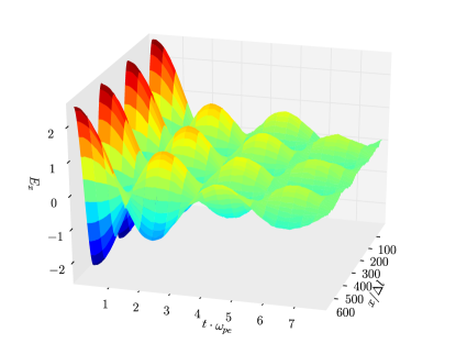
Figure 1: The time evolution of an electrostatic wave in a hot plasma.

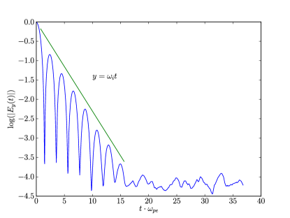
Figure 2: Logarithmic plot of the time evolution of absolute value of the electric field. The slope of the solid green line is the theoretical damping rate.

Another test problem is the dispersion relation of electron Bernstein waves Stix (1992). In this problem, an electromagnetic wave propagates perpendicularly to an uniform external magnetic field $\mathbf{B}_{0}=B_{0}\mathbf{e}_{z}$ with $B_{0}=5.13$T. Other system parameters are

$$n_{e} = 2.4\times 10^{20}\mathrm{m^{-3}}\leavevmode\nobreak\ ,$$ (67)

$$v_{T} = 0.07c\leavevmode\nobreak\ ,$$ (68)

$$\Delta l = 2.5\times 10^{-5}m\leavevmode\nobreak\ ,$$ (69)

$$\Delta t = \frac{\Delta l}{2c}\leavevmode\nobreak\ .$$ (70)

The computation domain is a $768\times 1\times 1$ cubic mesh, and the averaged number of sample points per grid is 4000. An initial electromagnetic perturbation is imposed, and after simulating 6000 time steps the space-time spectrum of $E_{x}$ is plotted in Fig. 3, which shows that the dispersion relation simulated matches the theoretical curve perfectly.

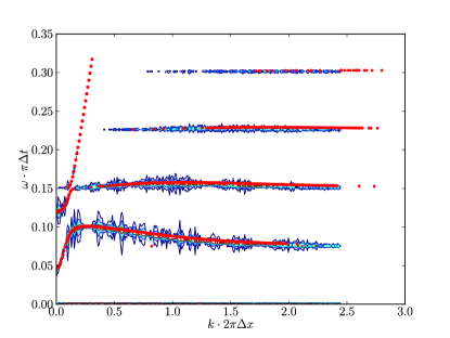
Figure 3: The dispersion relation of electron Bernstein wave (contours) obtained by the non-canonical symplectic PIC method. The red dots are calculated from the analytical dispersion relation.

As a symplectic method, the non-canonical symplectic PIC algorithm is expected to have good long-term properties. To demonstrate that, we run another test, where the system parameters are same as the previous problem for the Bernstein wave, except that the number of sample particles is 40 per grid and the simulation domain is a $48\times 1\times 1$ cubic mesh. Both the second order and the first order split methods are tested. The simulation is run for 2.5 million time-steps, and the evolution of total energy errors are plotted in Fig. 4. It is clear that the energy errors are bounded within a small value during the entire long-term simulation for both split methods, and the second order method is more accurate than the first order method.

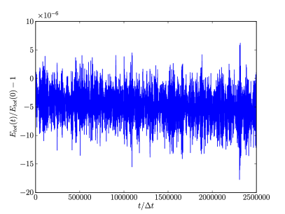
(a) Second order algorithm.

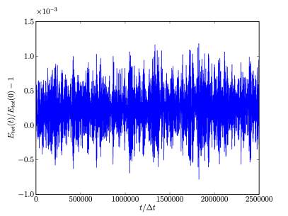
(b) First order algorithm.

Figure 4: Total energy error as a function of time for a magnetized hot plasma obtained by the second (a) and first (b) order non-canonical symplectic PIC method. Both energy errors are bounded within a small value.

IV Summary and Discussion

We have developed and tested a non-canonical symplectic PIC algorithm for the VM system. The non-canonical symplectic structure is obtained by discretizing the electromagnetic field of the particle-field Lagrangian using the method of discrete exterior calculus. A high-order interpolating method for differential forms is developed to render smooth interpolations of the electromagnetic field. The effectiveness and conservative nature of the algorithm has been verified by the physics problems of nonlinear Landau damping and electron Bernstein wave.

Appendix A High order interpolation forms for a cubic mesh

The interpolation forms for a cubic mesh is inspired by the Whitney forms Whitney (1957), which were originally developed as first order interpolation forms over simplicial complex and has become an important tool in discrete exterior calculus (DEC) Hirani (2003); Whitney (1957); Desbrun et al. (2008). In DEC theory, the discrete forms are defined on chains Hirani (2003). For example, discrete 0-forms are defined on vertexes of the grid, discrete 1-forms are defined on edges, and the discrete differential operators such as $\nabla_{d}$ and ${\mathrm{curl_{d}}}$ are discrete exterior derivatives $\mathbf{d}_{d}$ acted on these discrete forms. The Whitney map $\phi_{W}$ is a map that allows us to define continuous forms based on these discrete forms Hirani (2003). With this map, the following relation holds for any discrete form $\alpha$,

$$\phi_{W}\mathbf{d}_{d}\alpha=\mathbf{d}\phi_{W}\alpha\leavevmode\nobreak\ ,$$ (71)

where $\mathbf{d}$ is the continuous exterior derivative.

DEC solvers for Maxwell equations in cubic meshes are given by Stern, et al. Stern et al. (2015). For our purpose, we need to construct appropriate discrete differential operators $\nabla_{\mathrm{d}}$, ${\mathrm{curl_{d}}}$, ${\mathrm{div_{d}}}$ as well as interpolation functions $W_{\sigma_{0I}}\left(\mathbf{x}\right)$, $W_{\sigma_{1J}}\left(\mathbf{x}\right)$, $W_{\sigma_{2K}}\left(\mathbf{x}\right)$ and $W_{\sigma_{3L}}\left(\mathbf{x}\right)$ in a cubic mesh such that

$$\nabla\sum_{I}W_{\sigma_{0I}}\left(\mathbf{x}\right) \phi_{I}= \sum_{I,J}W_{\sigma_{1J}}\left(\mathbf{x}\right){\nabla_{\mathrm{d}}}_{JI}\phi_{I}\leavevmode\nobreak\ ,$$ (72)

$$\nabla\times\sum_{J}W_{\sigma_{1J}}\left(\mathbf{x}\right)\mathbf{A}_{J} = \sum_{J,K}W_{\sigma_{2K}}\left(\mathbf{x}\right){{\mathrm{curl_{d}}}}_{KJ}\mathbf{A}_{J}\leavevmode\nobreak\ ,$$ (73)

$$\nabla\cdot\sum_{K}W_{\sigma_{2K}}\left(\mathbf{x}\right)\mathbf{B}_{K} = \sum_{K,L}W_{\sigma_{3L}}\left(\mathbf{x}\right){{\mathrm{div_{d}}}}_{LK}\mathbf{B}_{K}\leavevmode\nobreak\ ,$$ (74)

hold for any $\phi_{I}$, $\mathbf{A}_{J}$, and $\mathbf{B}_{K}$.

To accomplish this goal, we start from choosing an interpolation function $W_{\sigma_{0I}}\left(\mathbf{x}\right)=W_{\sigma_{0}}\left(\mathbf{x}-\mathbf{x}_{I}\right)$ for 0-forms (e.g. scalar potential) as follows,

$$W_{\sigma_{0}}\left(\mathbf{x}\right)=W_{1}\left(x\right)W_{1}\left(y\right)W_{1}\left(z\right)\leavevmode\nobreak\ ,$$ (75)

where $\mathbf{x}_{I}$ is the coordinate of the $I$-th grid vertex and the cell size is chosen to be 1 for simplicity. It is required that $W_{1}\left(x\right)$ satisfies the following conditions,

$$W_{1}\left(x\right)=0,\quad\textrm{if }|x|>=1\leavevmode\nobreak\ ,$$ (76)

$$W_{1}\left(x\right)+W_{1}\left(x-1\right)=1,\quad\textrm{if }0\leq x<1\leavevmode\nobreak\ .$$ (77)

For example, $W_{1}$ can be chosen to be piece-wise linear over one grid cell, i.e.,

$$W_{1}\left(x\right) = \left\{\begin{array}[]{lc}0,&|x|\geq 1\leavevmode\nobreak\ ,\\ 1-|x|,&|x|<1\leavevmode\nobreak\ .\end{array}\right.$$ (80)

For $x,y,z$ in $[i^{\prime},i^{\prime}+1),[j^{\prime},j^{\prime}+1),[k^{\prime},k^{\prime}+1)$, the $x$ component of the left hand side of Eq. (72) $T_{x}$ is

$$T_{x} = \sum_{i\in\{i^{\prime},i^{\prime}+1\},j\in\{j^{\prime},j^{\prime}+1\},k\in\{k^{\prime},k^{\prime}+1\}}\phi_{i,j,k}W_{1}^{\prime}(x-i)W_{1}(y-j)W_{1}(z-k)$$ (81)

$$= \sum_{j\in\{j^{\prime},j^{\prime}+1\},k\in\{k^{\prime},k^{\prime}+1\}}\left(\phi_{i^{\prime},j,k}W_{1}^{\prime}(x-i^{\prime})+\phi_{i^{\prime}+1,j,k}W_{1}^{\prime}(x-i^{\prime}-1)\right)W_{1}(y-j)W_{1}(z-k)$$

$$= \sum_{j\in\{j^{\prime},j^{\prime}+1\},k\in\{k^{\prime},k^{\prime}+1\}}\left(\phi_{i^{\prime},j,k}-\phi_{i^{\prime}+1,j,k}\right)W_{1}^{\prime}(x-i^{\prime})W_{1}(y-j)W_{1}(z-k)\leavevmode\nobreak\ .$$

The $y$ and $z$ component can be also deduced in the similar way,

$$T_{y} = \sum_{i\in\{i^{\prime},i^{\prime}+1\},k\in\{k^{\prime},k^{\prime}+1\}}\left(\phi_{i,j^{\prime},k}-\phi_{i,j^{\prime}+1,k}\right)W_{1}(x-i)W_{1}^{\prime}(y-j^{\prime})W_{1}(z-k)\leavevmode\nobreak\ ,$$ (82)

$$T_{z} = \sum_{i\in\{i^{\prime},i^{\prime}+1\},j\in\{j^{\prime},j^{\prime}+1\}}\left(\phi_{i,j,k^{\prime}}-\phi_{i,j,k^{\prime}+1}\right)W_{1}(x-i)W_{1}(y-j)W_{1}^{\prime}(z-k^{\prime})\leavevmode\nobreak\ .$$ (83)

Equations (81)-(83) indicate that $W_{1}^{\prime}(x-i)W_{1}(y-j)W_{1}(z-k)dx$, $W_{1}(x-i)W_{1}^{\prime}(y-j)W_{1}(z-k)dy$, and $W_{1}(x-i)W_{1}(y-j)W_{1}^{\prime}(z-k)dz$ can be viewed as the bases for 1-form interpolation map, and that the discrete gradient operator $\nabla_{\mathrm{d}}$ can be defined as linear operator on $\phi_{I}$ as

$$\left({\nabla_{\mathrm{d}}}\phi\right)_{i,j,k}=[\phi_{i+1,j,k}-\phi_{i,j,k},\phi_{i,j+1,k}-\phi_{i,j,k},\phi_{i,j,k+1}-\phi_{i,j,k}]\leavevmode\nobreak\ .$$ (84)

For a given discrete 1-form field $\mathbf{A}_{I}$, the interpolated 1-form field is

$$\sum_{i,j,k}\left[{A_{x}}_{i,j,k}W_{1}^{(1)}(x-i)W_{1}(y-j)W_{1}(z-k)dx\right.\\ +{A_{y}}_{i,j,k}W_{1}(x-i)W_{1}^{(1)}(y-j)W_{1}(z-k)dy\\ \left.+{A_{z}}_{i,j,k}W_{1}(x-i)W_{1}(y-j)W_{1}^{(1)}(z-k)dz\right],$$ (85)

where

$$W_{1}^{(1)}\left(x\right)=\left\{\begin{array}[]{lc}-W_{1}^{\prime}(x),&0\leq x<1\leavevmode\nobreak\ ,\\ 0,&\textrm{otherwise}\leavevmode\nobreak\ .\end{array}\right.$$ (88)

is the one-cell interpolation function. The components of this interpolated 1-form field are written as

$$\sum_{i,j,k}W_{\sigma_{1,i,j,k}}\left(\mathbf{x}\right)\mathbf{A}_{i,j,k}\equiv\sum_{i,j,k}\left[\begin{array}[]{c}{A_{x}}_{i,j,k}W_{1}^{(1)}(x-i)W_{1}(y-j)W_{1}(z-k)\\ {A_{y}}_{i,j,k}W_{1}(x-i)W_{1}^{(1)}(y-j)W_{1}(z-k)\\ {A_{z}}_{i,j,k}W_{1}(x-i)W_{1}(y-j)W_{1}^{(1)}(z-k)\nobreak\leavevmode\end{array}\right]^{T}\leavevmode\nobreak\ .$$ (89)

By the same procedure, we find that discrete differential operators ${\mathrm{curl_{d}}}$ and ${\mathrm{div_{d}}}$ should be defined as

$$\left({{\mathrm{curl_{d}}}}\mathbf{A}\right)_{i,j,k}=\left[\begin{array}[]{c}\left({A_{z}}_{i,j+1,k}-{A_{z}}_{i,j,k}\right)-\left({A_{y}}_{i,j,k+1}-{A_{y}}_{i,j,k}\right)\\ \left({A_{x}}_{i,j,k+1}-{A_{x}}_{i,j,k}\right)-\left({A_{z}}_{i+1,j,k}-{A_{z}}_{i,j,k}\right)\\ \left({A_{y}}_{i+1,j,k}-{A_{y}}_{i,j,k}\right)-\left({A_{x}}_{i,j+1,k}-{A_{x}}_{i,j,k}\right)\end{array}\right]^{T}\leavevmode\nobreak\ ,$$ (93)

$$\left({{\mathrm{div_{d}}}}\mathbf{B}\right)_{i,j,k}=\left[\left({B_{x}}_{i+1,j,k}-{B_{x}}_{i,j,k}\right)+\left({B_{y}}_{i,j+1,k}-{B_{y}}_{i,j,k}\right)+\left({B_{z}}_{i,j,k+1}-{B_{z}}_{i,j,k}\right)\right]\leavevmode\nobreak\ .$$ (94)

For a given discrete 2-form field $\mathbf{B}_{I}$, the interpolated 2-form field is

$$\sum_{i,j,k}\left[{B_{x}}_{i,j,k}W_{1}(x-i)W_{1}^{(1)}(y-j)W_{1}^{(1)}(z-k)dy\land dz\right.\\ +{B_{y}}_{i,j,k}W_{1}^{(1)}(x-i)W_{1}(y-j)W_{1}^{(1)}(z-k)dz\land dx\\ \left.+{B_{z}}_{i,j,k}W_{1}^{(1)}(x-i)W_{1}^{(1)}(y-j)W_{1}(z-k)dx\land dy\right],$$ (95)

whose components can be written as

$$\sum_{i,j,k}W_{\sigma_{2,i,j,k}}\left(\mathbf{x}\right)\mathbf{B}_{i,j,k}\equiv\sum_{i,j,k}\left[\begin{array}[]{c}{B_{x}}_{i,j,k}W_{1}(x-i)W_{1}^{(1)}(y-j)W_{1}^{(1)}(z-k)\\ {B_{y}}_{i,j,k}W_{1}^{(1)}(x-i)W_{1}(y-j)W_{1}^{(1)}(z-k)\\ {B_{z}}_{i,j,k}W_{1}^{(1)}(x-i)W_{1}^{(1)}(y-j)W_{1}(z-k)\end{array}\right]^{T}.$$ (96)

For a discrete 3-form field $\rho_{I}$, the interpolated 3-form field is

$$\sum_{i,j,k}\rho_{i,j,k}W_{1}^{(1)}(x-i)W_{1}^{(1)}(y-j)W_{1}^{(1)}(z-k)dx\land dy\land dz\leavevmode\nobreak\ ,$$ (97)

and the corresponding scaler is denoted as

$$\sum_{i,j,k}W_{\sigma_{3,i,j,k}}\left(\mathbf{x}\right)\rho_{i,j,k}\equiv\sum_{i,j,k}\rho_{i,j,k}W_{1}^{(1)}(x-i)W_{1}^{(1)}(y-j)W_{1}^{(1)}(z-k)\leavevmode\nobreak\ .$$ (98)

We can verify that

$$\left({\mathrm{curl_{d}}}\nabla_{\mathrm{d}}\phi\right)_{i,j,k}=0,\quad\textrm{for any }i,j,k\textrm{ and }\phi\leavevmode\nobreak\ ,$$ (99)

$$\left({\mathrm{div_{d}}}{\mathrm{curl_{d}}}\mathbf{A}\right)_{i,j,k}=0,\quad\textrm{for any }i,j,k\textrm{ and }\mathbf{A}\leavevmode\nobreak\ .$$ (100)

In Ref. Stern et al. (2015) the discrete electromagnetic fields in cubic mesh seem different from ours on first look. But the difference is merely in the notation for indices. For example, for discrete 1-form, we can alternatively use half-integer indices to rewrite Eq. (84) as

$$[\left({\nabla_{\mathrm{d}}}\phi\right)_{xi+1/2,j,k},\left({\nabla_{\mathrm{d}}}\phi\right)_{yi,j+1/2,k},\left({\nabla_{\mathrm{\mathrm{d}}}}\phi\right)_{zi,j,k+1/2}]=$$

$$[\phi_{i+1,j,k}-\phi_{i,j,k},\phi_{i,j+1,k}-\phi_{i,j,k},\phi_{i,j,k+1}-\phi_{i,j,k}]\leavevmode\nobreak\ ,$$ (101)

which is then identical with the notation in Ref. Stern et al. (2015).

The above interpolation forms are defined over one grid cell. For the simulations reported here, in order to achieve higher accuracy, we have developed and deployed high-order interpolation forms over two grid cells. The interpolation 0-forms are

$$W_{\sigma_{0}}\left(\mathbf{x}\right)=W_{1}\left(x\right)W_{1}\left(y\right)W_{1}\left(z\right)\leavevmode\nobreak\ ,$$ (102)

where $W_{1}\left(x\right)$ satisfies

$$W_{1}\left(x\right) = 0,\quad\textrm{if }|x|>=2\leavevmode\nobreak\ ,$$ (103)

$$W_{1}\left(x+1\right)+W_{1}\left(x\right)+W_{1}\left(x-1\right)+W_{1}\left(x-2\right) = 1,\quad\textrm{if }0\leq x<1\leavevmode\nobreak\ .$$ (104)

The $W_{1}$ adopted in the algorithm is

$$W_{1}\left(x\right)=\left\{\begin{array}[]{lc}0\leavevmode\nobreak\ ,&x>2\leavevmode\nobreak\ ,\\ \frac{15}{1024}x^{8}-\frac{15}{128}x^{7}+\frac{49}{128}x^{6}-\frac{21}{32}x^{5}+\frac{35}{64}x^{4}-x+1\leavevmode\nobreak\ ,&1<x\leq 2\leavevmode\nobreak\ ,\\ -\frac{15}{1024}x^{8}-\frac{15}{128}x^{7}+\frac{7}{16}x^{6}-\frac{21}{32}x^{5}+\frac{175}{256}x^{4}-\frac{105}{128}x^{2}+\frac{337}{512}\leavevmode\nobreak\ ,&0<x\leq 1\leavevmode\nobreak\ ,\\ -\frac{15}{1024}x^{8}+\frac{15}{128}x^{7}+\frac{7}{16}x^{6}+\frac{21}{32}x^{5}+\frac{175}{256}x^{4}-\frac{105}{128}x^{2}+\frac{337}{512}\leavevmode\nobreak\ ,&-1<x\leq 0\leavevmode\nobreak\ ,\\ \frac{15}{1024}x^{8}+\frac{15}{128}x^{7}+\frac{49}{128}x^{6}+\frac{21}{32}x^{5}+\frac{35}{64}x^{4}+x+1\leavevmode\nobreak\ ,&-2<x\leq-1\leavevmode\nobreak\ ,\\ 0\leavevmode\nobreak\ ,&x\leq-2\leavevmode\nobreak\ .\end{array}\right.$$ (111)

It can be proved that this piece-wise polynomial function is 3rd order continuous in the whole space. For this two-cell interpolation scheme, the $\nabla_{\mathrm{d}}$ defined in Eq. (84), ${\mathrm{curl_{d}}}$ defined in Eq. (93), and ${\mathrm{div_{d}}}$ defined in Eq. (94) remain the same, but the function $W_{1}^{(1)}$ in Eqs. (85), (89), (95), (96), (97) and (98) needs to be replaced by the $W_{1}^{(2)}$ function defined as

$$W_{1}^{(2)}\left(x\right)=-\left\{\begin{array}[]{lc}W_{1}^{\prime}\left(x\right)+W_{1}^{\prime}\left(x+1\right)+W_{1}^{\prime}\left(x+2\right)\leavevmode\nobreak\ ,&-1\leq x<2\leavevmode\nobreak\ ,\\ 0\leavevmode\nobreak\ ,&\mathrm{otherwise}\leavevmode\nobreak\ .\end{array}\right.$$ (114)

It can be proved that Eqs. (72), (73), (74), (99), and (100) hold for this two-cell interpolation scheme.