The partial vine copula: A dependence measure and approximation based on the simplifying assumption

Abstract

Simplified vine copulas (SVCs), or pair-copula constructions, have become an important tool in high-dimensional dependence modeling. So far, specification and estimation of SVCs has been conducted under the simplifying assumption, i.e., all bivariate conditional copulas of the vine are assumed to be bivariate unconditional copulas. We introduce the partial vine copula (PVC) which provides a new multivariate dependence measure and which plays a major role in the approximation of multivariate distributions by SVCs. The PVC is a particular SVC where to any edge a $j$-th order partial copula is assigned and constitutes a multivariate analogue of the bivariate partial copula. We investigate to what extent the PVC describes the dependence structure of the underlying copula. We show that the PVC does not minimize the Kullback-Leibler divergence from the true copula and that the best approximation satisfying the simplifying assumption is given by a vine pseudo-copula. However, under regularity conditions, stepwise estimators of pair-copula constructions converge to the PVC irrespective of whether the simplifying assumption holds or not. Moreover, we elucidate why the PVC is the best feasible SVC approximation in practice.

note showproof

and c1Corresponding author.

1 Introduction

Copulas constitute an important tool to model dependence [1, 2, 3]. While it is easy to construct bivariate copulas, the construction of flexible high-dimensional copulas is a sophisticated problem. The introduction of simplified vine copulas (Joe [4]), or pair-copula constructions (Aas et al. [5]), has been an enormous advance for high-dimensional dependence modeling. Simplified vine copulas are hierarchical structures, constructed upon a sequence of bivariate unconditional copulas, which capture the conditional dependence between pairs of random variables if the data generating process satisfies the simplifying assumption. In this case, all conditional copulas of the data generating vine collapse to unconditional copulas and the true copula can be represented in terms of a simplified vine copula. Vine copula methodology and application have been extensively developed under the simplifying assumption [6, 7, 8, 9, 10], with studies showing the superiority of simplified vine copula models over elliptical copulas and nested Archimedean copulas (Aas and Berg [11], Fischer et al. [12]).

Although some copulas can be expressed as a simplified vine copula, the simplifying assumption is not true in general. Hobæk Haff et al. [13] point out that the simplifying assumption is in general not valid and provide examples of multivariate distributions which do not satisfy the simplifying assumption. Stöber et al. [14] show that the Clayton copula is the only Archimedean copula for which the simplifying assumption holds, while the Student-t copula is the only simplified vine copula arising from a scale mixture of normal distributions. In fact, it is very unlikely that the unknown data generating process satisfies the simplifying assumption in a strict mathematical sense. As a result, researchers have recently started to investigate new dependence concepts that are related to the simplifying assumption and arise if it does not hold. In particular, studies on the bivariate partial copula, a generalization of the partial correlation coefficient, have (re-)emerged lately [15, 16, 17, 18, 19].

We introduce the partial vine copula (PVC) which constitutes a multivariate analogue of the bivariate partial copula and which generalizes the partial correlation matrix. The PVC is a particular simplified vine copula where to any edge a $j$-th order partial copula is assigned. It provides a new multivariate dependence measure for a $d$-dimensional random vector in terms of $d(d-1)/2$ bivariate unconditional copulas and can be readily estimated for high-dimensional data [20]. We investigate several properties of the PVC and show to what extent the dependence structure of the underlying distribution is captured. The PVC plays a crucial role in terms of approximating a multivariate distribution by a simplified vine copula (SVC). We show that many estimators of SVCs converge to the PVC if the simplifying assumption does not hold. However, we also prove that the PVC may not minimize the Kullback-Leibler divergence from the true copula and thus may not be the best approximation in the space of simplified vine copulas. This result is rather surprising, because it implies that it may not be optimal to specify the true copulas in the first tree of a simplified vine copula approximation. Moreover, joint and stepwise estimators of SVCs may not converge to the same probability limit any more if the simplifying assumption does not hold. Nevertheless, due to the prohibitive computational burden or simply because only a stepwise model selection and estimation is possible, the PVC is the best feasible SVC approximation in practice. Moreover, the PVC is used by [20] to construct a new non-parametric estimator of a multivariate distribution that can outperform classical non-parametric approaches and by [21] to test the simplifying assumption in high-dimensional vine copulas. All in all, these facts highlight the great practical importance of the PVC for multivariate dependence modeling.

The rest of this paper is organized as follows. (Simplified) vine copulas, the simplifying assumption, conditional and partial copulas, are discussed in Section 2. The PVC and $j$-th order partial copulas are introduced in Section 3. Properties of the PVC and some examples are presented in Section 4. In Section 5 we analyze the role of the PVC for simplified vine copula approximations and explain why the PVC is the best feasible approximation in practical applications. A parametric estimator for the PVC is presented in Section 6 and implications for the stepwise and joint maximum likelihood estimator of simplified vine copulas are illustrated. Section 7 contains some concluding remarks.

The following notation and assumptions are used throughout the paper. We write $X_{1:d}:=(X_{1},\ldots,X_{d})$, so that $F_{X_{1:d}}(x_{1:d}):=\mathbb{P}(\forall i=1,\ldots,d\colon X_{i}\leq x_{i})$, and $\text{d}x_{1:d}:=\text{d}x_{1}\ldots\text{d}x_{d}$ to denote the variables of integration in $\int f_{X_{1:d}}(x_{1:d})\text{d}x_{1:d}$. $C^{\perp}$ refers to the independence copula. $X\perp Y$ means that $X$ and $Y$ are stochastically independent. For $1\leq k\leq d$, the partial derivative of $g$ w.r.t. the $k$-th argument is denoted by $\partial_{k}g(x_{1:d})$. We write $1\!\!1_{\{A\}}=1$ if $A$ is true, and $1\!\!1_{\{A\}}=0$ otherwise. For simplicity, we assume that all random variables are real-valued and continuous. In the following, let $d\geq 3$, if not otherwise specified, and ${\cal C}_{d}$ be the space of absolutely continuous $d$-dimensional copulas with positive density (a.s.). The distribution function of a random vector $U_{1:d}$ with uniform margins is denoted by $F_{1:d}=C_{1:d}\in{\cal C}_{d}$. We set ${\cal I}_{l}^{d}:=\{(i,j)\colon j=l,\ldots,d-1,i=1,\ldots,d-j\}$ and $S_{ij}:=i+1:i+j-1:=i+1,\ldots,i+j-1$. We focus on D-vine copulas, but all results carry over to regular vine copulas (Bedford and Cooke [22], Kurowicka and Joe [23]). An overview of the used notation can be found in Table 1. All proofs are deferred to the appendix.

Table 1: Notation for simplified D-vine copulas. $U_{1:d}$ has standard uniform margins, $d\geq 3,(i,j)\in{\cal I}_{1}^{d},k=i,i+j$.

Notation	Explanation
$F_{1:d}$ or $C_{1:d}$	cdf and copula of $U_{1:d}$
${\cal C}_{d}$	space of $d$-dimensional copulas with positive density
${\cal C}^{\text{\tiny SVC}}_{d}$	space of $d$-dimensional simplified D-vine copulas with positive density
${\cal I}_{1}^{d}$	${\cal I}_{1}^{d}:=\{(i,j)\colon j=1,\ldots,d-1,i=1,\ldots,d-j\}$, the conditioned set of a D-vine copula density
$S_{ij}$	$S_{ij}:=i+1:i+j-1:=i+1,\ldots,i+j-1$, the conditioning set of an edge in a D-vine
$U_{k|S_{ij}}$	$F_{k|S_{ij}}(U_{k}|U_{S_{ij}})$, conditional probability integral transform (CPIT) of $U_{k}$ w.r.t. $U_{S_{ij}}$
$C_{i,i+j;\kern 0.448ptS_{ij}}$	bivariate conditional copula of $F_{i,{i+j}|{S_{ij}}}$, i.e., $C_{i,i+j;\kern 0.448ptS_{ij}}=F_{U_{i|S_{ij}},U_{i+j|S_{ij}}|U_{S_{ij}}}$
$C^{\text{\tiny SVC}}_{i,i+j;\kern 0.448ptS_{ij}}$	arbitrary bivariate (unconditional) copula that is used to model $C_{i,i+j;\kern 0.448ptS_{ij}}$
$C^{\text{\tiny P}}_{i,i+j;\kern 0.448ptS_{ij}}$	partial copula of $C_{i,i+j;\kern 0.448ptS_{ij}}$, i.e., $C^{\text{\tiny P}}_{i,i+j;\kern 0.448ptS_{ij}}=F_{U_{i|S_{ij}},U_{i+j|S_{ij}}}$
$C^{\text{\tiny PVC}}_{i,i+j;\kern 0.448ptS_{ij}}$	$(j-1)$-th order partial copula of $C_{i,i+j;\kern 0.448ptS_{ij}}$
$U^{\text{\tiny PVC}}_{k|S_{ij}}$	$F^{\text{\tiny PVC}}_{k|S_{ij}}(U_{k}|U_{S_{ij}})$, $(j\!-\!2)$-th order partial probability integral transform (PPIT) of $U_{k}$ w.r.t. $U_{S_{ij}}$
$C^{\text{\tiny PVC}}_{1:d}$	Partial vine copula (PVC) of $C_{1:d}$, if $d=3$, then $c^{\text{\tiny PVC}}_{1:3}(u_{1:3})=c_{12}(u_{1},u_{2})\ \!c_{23}(u_{2},u_{3})\ \!c^{\text{\tiny PVC}}_{13;\kern 0.448pt2}(u_{1|2},u_{3|2})$

2 Simplified vine copulas, conditional copulas, and higher-order partial copulas

In this section, we discuss (simplified) vine copulas and the simplifying assumption. Thereafter, we introduce the partial copula which can be considered as a generalization of the partial correlation coefficient and as an approximation of a bivariate conditional copula.

Definition 2.1 (Simplified D-vine copula or pair-copula construction – Joe [4], Aas et al. [5])

For $(i,j)\in{\cal I}_{1}^{d}$, let $C^{\text{\tiny SVC}}_{i,i+j;\kern 0.56001ptS_{ij}}\in{\cal C}_{2}$ with density $c^{\text{\tiny SVC}}_{i,i+j;\kern 0.56001ptS_{ij}}$. For $j=1$ and $i=1,\ldots,d-j$, we set $C^{\text{\tiny SVC}}_{i,i+j;\kern 0.56001ptS_{ij}}=C^{\text{\tiny SVC}}_{i,i+1}$ and $u^{\text{\tiny SVC}}_{k|S_{ij}}=u_{k}$ for $k=i,i+j$. For $(i,j)\in{\cal I}_{2}^{d}$, define

$$u^{\text{\tiny SVC}}_{i|S_{ij}}:=F^{\text{\tiny SVC}}_{i|S_{ij}}(u_{i}|u_{S_{ij}}) =\partial_{2}C^{\text{\tiny SVC}}_{i,i+j-1;\kern 0.56001ptS_{i,j-1}}(u^{\text{\tiny SVC}}_{i|S_{i,j-1}},u^{\text{\tiny SVC}}_{i+j-1|S_{i,j-1}}),$$

$$u^{\text{\tiny SVC}}_{i+j|S_{ij}}:=F^{\text{\tiny SVC}}_{i+j|S_{ij}}(u_{i+j}|u_{S_{ij}}) =\partial_{1}C^{\text{\tiny SVC}}_{i+1,i+j;\kern 0.56001ptS_{i+1,j-1}}(u^{\text{\tiny SVC}}_{i+1|S_{i+1,j-1}},u^{\text{\tiny SVC}}_{i+j|S_{i+1,j-1}}).$$

Then

$$c^{\text{\tiny SVC}}_{1:d}(u_{1:d}) =\prod_{(i,j)\in{\cal I}_{1}^{d}}c^{\text{\tiny SVC}}_{i,i+j;\kern 0.56001ptS_{ij}}\big{(}u^{\text{\tiny SVC}}_{i|S_{ij}},u^{\text{\tiny SVC}}_{i+j|S_{ij}}\big{)}$$

is the density of a $d$-dimensional simplified D-vine copula $C^{\text{\tiny SVC}}_{1:d}$. We denote the space of $d$-dimensional simplified D-vine copulas by ${\cal C}^{\text{\tiny SVC}}_{d}$.

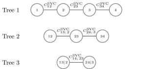
(a) Simplified D-vine copula.

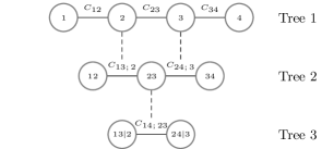
(b) D-vine copula.

Figure 1: (Simplified) D-vine copula representation if $d=4$. The influence of conditioning variables on the conditional copulas is indicated by dashed lines.

From a graph-theoretic point of view, simplified (regular) vine copulas can be considered as an ordered sequence of trees, where $j$ refers to the number of the tree and a bivariate unconditional copula $C^{\text{\tiny SVC}}_{i,i+j;\kern 0.56001ptS_{ij}}$ is assigned to each of the $d-j$ edges of tree $j$ (Bedford and Cooke [22]). The left hand side of Figure 1 shows the graphical representation of a simplified D-vine copula for $d=4$, i.e.,

$$c^{\text{\tiny SVC}}_{1:4}(u_{1:4}) =\underbrace{c^{\text{\tiny SVC}}_{12}(u_{1},u_{2})c^{\text{\tiny SVC}}_{23}(u_{2},u_{3})c^{\text{\tiny SVC}}_{34}(u_{3},u_{4})}_{\text{first tree}}\times\underbrace{c^{\text{\tiny SVC}}_{13;\kern 0.56001pt2}(u^{\text{\tiny SVC}}_{1|2},u^{\text{\tiny SVC}}_{3|2})c^{\text{\tiny SVC}}_{24;\kern 0.56001pt3}(u^{\text{\tiny SVC}}_{2|3},u^{\text{\tiny SVC}}_{4|3})}_{\text{second tree}}\times\underbrace{c^{\text{\tiny SVC}}_{14;\kern 0.56001pt2:3}(u^{\text{\tiny SVC}}_{1|2:3},u^{\text{\tiny SVC}}_{4|2:3})}_{\text{third tree}}.$$

The bivariate unconditional copulas $C^{\text{\tiny SVC}}_{i,i+j;\kern 0.56001ptS_{ij}}$ are also called pair-copulas, so that the resulting model is often termed a pair-copula construction (PCC). By means of simplified vine copula models one can construct a wide variety of flexible multivariate copulas because each of the $d(d-1)/2$ bivariate unconditional copulas $C^{\text{\tiny SVC}}_{i,i+j;\kern 0.56001ptS_{ij}}$ can be chosen arbitrarily and the resulting model is always a valid $d$-dimensional copula. Moreover, a pair-copula construction does not suffer from the curse of dimensions because it is build upon a sequence of bivariate unconditional copulas which renders it very attractive for high-dimensional applications. Obviously, not every multivariate copula can be represented by a simplified vine copula. However, every copula can be represented by the following (non-simplified) D-vine copula.

Definition 2.2 (D-vine copula – Kurowicka and Cooke [24])

Let $U_{1:d}$ be a random vector with cdf $F_{1:d}=C_{1:d}\in{\cal C}_{d}$. For $j=1$ and $i=1,\ldots,d-j$, we set ${C}_{i,i+j;\kern 0.56001ptS_{ij}}={C}_{i,i+1}$ and ${u}_{k|S_{ij}}=u_{k}$ for $k=i,i+j$. For $(i,j)\in{\cal I}_{2}^{d}$, let $C_{i,i+j;\kern 0.56001ptS_{ij}}$ denote the conditional copula of $F_{i,i+j|S_{ij}}$ (Definition 2.5) and let $u_{k|S_{ij}}:=F_{k|S_{ij}}(u_{k}|u_{S_{ij}})$ for $k=i,i+j$. The density of a D-vine copula decomposes the copula density of $U_{1:d}$ into $d(d-1)/2$ bivariate conditional copula densities $c_{i,i+j;\kern 0.56001ptS_{ij}}$ according to the following factorization:

$$c_{1:d}(u_{1:d}) =\prod_{(i,j)\in{\cal I}_{1}^{d}}c_{i,i+j;\kern 0.56001ptS_{ij}}(u_{i|{S_{ij}}},u_{i+j|S_{ij}}|u_{S_{ij}}).$$

Contrary to a simplified D-vine copula in Definition 2.1, a bivariate conditional copula $C_{i,i+j;\kern 0.56001ptS_{ij}}$, which is in general a function of $j+1$ variables, is assigned to each edge of a D-vine copula in Definition 2.2. The influence of the conditioning variables on the conditional copulas is illustrated by dashed lines in the right hand side of Figure 1. In applications, the simplifying assumption is typically imposed, i.e., it is assumed that all bivariate conditional copulas of the data generating vine copula degenerate to bivariate unconditional copulas.

Definition 2.3 (The simplifying assumption – Hobæk Haff et al. [13])

The D-vine copula in Definition 2.2 satisfies the simplifying assumption if $c_{i,i+j;\kern 0.56001ptS_{ij}}(\cdot,\cdot|u_{S_{ij}})$ does not depend on $u_{S_{ij}}$ for all $(i,j)\!\in\!{\cal I}_{2}^{d}$.

If the data generating copula satisfies the simplifying assumption, it can be represented by a simplified vine copula, resulting in fast and simple statistical inference. Several methods for the consistent specification and estimation of pair-copula constructions have been developed under this assumption (Hobæk Haff [25], Dißmann et al. [6]). However, in view of Definition 2.2 and Definition 2.1 it is evident that it is extremely unlikely that the data generating vine copula strictly satisfies the simplifying assumption in practical applications.

Several questions arise if the data generating process does not satisfy the simplifying assumption and a simplified D-vine copula model (Definition 2.1) is used to approximate a general D-vine copula (Definition 2.2). First of all, what bivariate unconditional copulas $C^{\text{\tiny SVC}}_{i,i+j;\kern 0.56001ptS_{ij}}$ should be chosen in Definition 2.1 to model the bivariate conditional copulas $C_{i,i+j;\kern 0.56001ptS_{ij}}$ in Definition 2.2 so that the best approximation w.r.t. a certain criterion is obtained? What simplified vine copula model do established stepwise procedures (asymptotically) specify and estimate if the simplifying assumption does not hold for the data generating vine copula? What are the properties of an optimal approximation? Before we address these questions in Section 5, it is useful to recall the definition of the conditional and partial copula in the remainder of this section and to introduce and investigate the partial vine copula in Section 3 and Section 4 because it plays a major role in the approximation of copulas by simplified vine copulas.

Definition 2.4 (Conditional probability integral transform (CPIT))

Let $U_{1:d}\sim F_{1:d}\in{\cal C}_{d}$, $(i,j)\in{\cal I}_{2}^{d}$ and $k=i,i+j$. We call $U_{k|S_{ij}}:=F_{k|S_{ij}}(U_{k}|U_{S_{ij}})$ the conditional probability integral transform of $U_{k}$ w.r.t. $U_{S_{ij}}$.

It can be readily verified that, under the assumptions in Definition 2.4, $U_{k|S_{ij}}\sim{\cal U}(0,1)$ and $U_{k|S_{ij}}\perp U_{S_{ij}}$. Thus, applying the random transformation $F_{k|S_{ij}}(\cdot|U_{S_{ij}})$ to $U_{k}$ removes possible dependencies between $U_{k}$ and $U_{S_{ij}}$ and $U_{k|S_{ij}}$ can be interpreted as the remaining variation in $U_{k}$ that can not be explained by $U_{S_{ij}}$. This interpretation of the CPIT is crucial for understanding the conditional and partial copula which are related to the (conditional) joint distribution of CPITs. The conditional copula has been introduced by Patton [26] and we restate its definition here.

Definition 2.5 (Bivariate conditional copula – Patton [26])

Let $U_{1:d}\sim F_{1:d}\in{\cal C}_{d}$ and $(i,j)\in{\cal I}_{2}^{d}$. The (a.s.) unique conditional copula $C_{i,i+j;\kern 0.56001ptS_{ij}}$ of the conditional distribution $F_{i,{i+j}|{S_{ij}}}$ is defined by

$$C_{i,i+j;\kern 0.56001ptS_{ij}}(a,b|u_{S_{ij}}) :=\mathbb{P}(U_{i|S_{ij}}\leq a,U_{i+j|S_{ij}}\leq b|U_{S_{ij}}=u_{S_{ij}})$$

$$\phantom{:}=F_{i,{i+j}|S_{ij}}(F_{i|{S_{ij}}}^{-1}(a|u_{S_{ij}}),F_{{i+j}|{S_{ij}}}^{-1}(b|u_{S_{ij}})|u_{S_{ij}}).$$

Equivalently, we have that

$$F_{i,{i+j}|{S_{ij}}}(u_{i},u_{i+j}|u_{S_{ij}})=C_{i,i+j;\kern 0.56001ptS_{ij}}(F_{i|{S_{ij}}}(u_{i}|u_{S_{ij}}),F_{{i+j}|{S_{ij}}}(u_{i+j}|u_{S_{ij}})|u_{S_{ij}}),$$

so that the effect of a change in $u_{S_{ij}}$ on the conditional distribution $F_{i,{i+j}|{S_{ij}}}(u_{i},u_{i+j}|u_{S_{ij}})$ can be separated into two effects. First, the values of the CPITs, $(F_{i|{S_{ij}}}(u_{i}|u_{S_{ij}}),F_{{i+j}|{S_{ij}}}(u_{i+j}|u_{S_{ij}}))$, at which the conditional copula is evaluated, may change. Second, the functional form of the conditional copula $C_{i,i+j;\kern 0.56001ptS_{ij}}(\cdot,\cdot|u_{S_{ij}})$ may vary. In comparison to the conditional copula, which is the conditional distribution of two CPITs, the partial copula is the unconditional distribution and copula of two CPITs.

Definition 2.6 (Bivariate partial copula - Bergsma [15])

Let $U_{1:d}\sim F_{1:d}\in{\cal C}_{d}$ and $(i,j)\in{\cal I}_{2}^{d}$. The partial copula $C^{\text{\tiny P}}_{i,i+j;\kern 0.56001ptS_{ij}}$ of the distribution $F_{i,{i+j}|{S_{ij}}}$ is defined by

$$C^{\text{\tiny P}}_{i,i+j;\kern 0.56001ptS_{ij}}(a,b) :=\mathbb{P}(U_{i|S_{ij}}\leq a,U_{i+j|S_{ij}}\leq b).$$

Since $U_{i|S_{ij}}\perp U_{S_{ij}}$ and $U_{i+j|S_{ij}}\perp U_{S_{ij}}$, the partial copula represents the distribution of random variables which are individually independent of the conditioning vector $U_{S_{ij}}$. This is similar to the partial correlation coefficient, which is the correlation of two random variables from which the linear influence of the conditioning vector has been removed. The partial copula can also be interpreted as the expected conditional copula,

$$C^{\text{\tiny P}}_{i,i+j;\kern 0.56001ptS_{ij}}(a,b)=\int_{\mathbb{R}^{j-1}}C_{i,i+j;\kern 0.56001ptS_{ij}}(a,b|u_{S_{ij}})\text{d}F_{{S_{ij}}}(u_{S_{ij}}),$$

and be considered as an approximation of the conditional copula. Indeed, it is easy to show that the partial copula $C^{\text{\tiny P}}_{i,i+j;\kern 0.56001ptS_{ij}}$ minimizes the Kullback-Leibler divergence from the conditional copula $C_{i,i+j;\kern 0.56001ptS_{ij}}$ in the space of absolutely continuous bivariate distribution functions. The partial copula is first mentioned by Bergsma [15] who applies the partial copula to test for conditional independence. Recently, there has been a renewed interest in the partial copula. Spanhel and Kurz [18] investigate properties of the partial copula and mention some explicit examples whereas Gijbels et al. [16, 17] and Portier and Segers [19] focus on the non-parametric estimation of the partial copula.

3 Higher-order partial copulas and the partial vine copula

A generalization of the partial correlation coefficient that is different from the partial copula is given by the higher-order partial copula. To illustrate this relation, let us recall the common definition of the partial correlation coefficient. Assume that all univariate margins of $Y_{1:d}$ have zero mean and finite variance. For $k=i,i+j$, let ${\cal P}(Y_{k}|Y_{S_{ij}})$ denote the best linear predictor of $Y_{k}$ w.r.t $Y_{S_{ij}}$ which minimizes the mean squared error so that $\tilde{{\cal E}}_{k|{S_{ij}}}=Y_{k}-{\cal P}(Y_{k}|Y_{S_{ij}})$ is the corresponding prediction error. The partial correlation coefficient of $Y_{i}$ and $Y_{i+j}$ given $Y_{S_{ij}}$ is then defined by $\rho_{i,i+j;S_{ij}}=\mathbb{C}\text{orr}[\tilde{{\cal E}}_{i|{S_{ij}}},\tilde{{\cal E}}_{{i+j}|{S_{ij}}}]$. An equivalent definition is given as follows. For $i=1,\ldots,d-2$, let

$$\begin{split}{\cal E}_{i|i+1}:=Y_{i}-{\cal P}(Y_{i}|Y_{i+1}),\quad&\text{and}\quad{\cal E}_{i+2|i+1}:=Y_{i+2}-{\cal P}(Y_{i+2}|Y_{i+1}).\end{split}$$ (3.1)

Moreover, for $j=3,\ldots,d-1$, and $i=1,\ldots,d-j$, define

$$\begin{split}{\cal E}_{i|S_{ij}}&:={\cal E}_{i|S_{i,j-1}}-{\cal P}({\cal E}_{i|S_{i,j-1}}|{\cal E}_{i+j-1|S_{i,j-1}}),\\ {\cal E}_{i+j|S_{ij}}&:={\cal E}_{i+j|S_{i+1,j-1}}-{\cal P}({\cal E}_{i+j|S_{i+1,j-1}}|{\cal E}_{i+1|S_{i+1,j-1}}).\end{split}$$ (3.2)

It is easy to show that ${\cal E}_{k|S_{ij}}=\tilde{{\cal E}}_{k|S_{ij}}$ for all $k=i,i+j$ and $(i,j)\in{\cal I}_{2}^{d}$. That is, ${\cal E}_{k|S_{ij}}$ is the error of the best linear prediction of $Y_{k}$ in terms of $Y_{S_{ij}}$. Thus, $\rho_{i,i+j;S_{ij}}=\mathbb{C}\text{orr}[{{\cal E}}_{i|S_{ij}},{\cal E}_{i+j|S_{ij}}]$. However, the interpretation of the partial correlation coefficient as a measure of conditional dependence is different depending on whether one considers it as the correlation of $(\tilde{{\cal E}}_{i|S_{ij}},\tilde{\cal E}_{i+j|S_{ij}})$ or $({{\cal E}}_{i|S_{ij}},{\cal E}_{i+j|S_{ij}})$. For instance, $\rho_{14;23}=\mathbb{C}\text{orr}[\tilde{\cal E}_{1|23},\tilde{\cal E}_{4|23}]$ can be interpreted as the correlation between $Y_{1}$ and $Y_{4}$ after each variable has been corrected for the linear influence of $Y_{2:3}$, i.e., $\mathbb{C}\text{orr}[g(\tilde{{\cal E}}_{k|23}),h(Y_{2:3})]=0$ for all linear functions $g$ and $h$. The idea of the partial copula is to replace the prediction errors ${\cal E}_{1|23}$ and ${\cal E}_{4|23}$ by the CPITS $U_{1|23}$ and $U_{4|23}$ which are independent of $Y_{2:3}$. On the other side, $\rho_{14;23}=\mathbb{C}\text{orr}\left[{\cal E}_{1|23},{\cal E}_{4|23}\right]$ is the correlation of $({\cal E}_{1|2},{\cal E}_{4|3})$ after ${\cal E}_{1|2}$ has been corrected for the linear influence of ${\cal E}_{3|2}$, and ${\cal E}_{4|3}$ has been corrected for the linear influence of ${\cal E}_{2|3}$. Consequently, a different generalization of the partial correlation coefficient emerges if we do not only decorrelate the involved random variables in (3.1) and (3.2) but render them independent by replacing each expression of the form $X-{\cal P}(X|Z)$ in (3.1) and (3.2) by the corresponding CPIT $F_{X|Z}(X|Z)$. The joint distribution of a resulting pair of random variables is given by the $j$-th order partial copula and the set of these copulas together with a vine structure constitute the partial vine copula.

Definition 3.1 (Partial vine copula (PVC) and $j$-th order partial copulas)

Consider the D-vine copula $C_{1:d}\in{\cal C}_{d}$ stated in Definition 2.2. In the first tree, we set for $i=1,\ldots,d-1\colon$ $C^{\text{\tiny PVC}}_{i,i+1}=C_{i,i+1},$ while in the second tree, we denote for $i=1,\ldots,d-2,k=i,i+2\colon C^{\text{\tiny PVC}}_{i,i+2;\kern 0.56001pti+1}=C^{\text{\tiny P}}_{i,i+2;\kern 0.56001pti+1}$ and $U^{\text{\tiny PVC}}_{k|i+1}=U_{k|i+1}=F_{k|i+1}(U_{k}|U_{i+1}).$ In the remaining trees $j=3,\ldots,d-1,$ for $i=1,\ldots,d-j$, we define

$$U^{\text{\tiny PVC}}_{i|S_{ij}}:=F^{\text{\tiny PVC}}_{i|S_{ij}}(U_{i}|U_{S_{ij}}) :=\partial_{2}C^{\text{\tiny PVC}}_{i,i+j-1;\kern 0.56001ptS_{i,j-1}}(U^{\text{\tiny PVC}}_{i|S_{i,j-1}},U^{\text{\tiny PVC}}_{i+j-1|S_{i,j-1}}),$$

$$U^{\text{\tiny PVC}}_{i+j|S_{ij}}:=F^{\text{\tiny PVC}}_{i+j|S_{ij}}(U_{i+j}|U_{S_{ij}}) :=\partial_{1}C^{\text{\tiny PVC}}_{i+1,i+j;\kern 0.56001ptS_{i+1,j-1}}(U^{\text{\tiny PVC}}_{i+1|S_{i+1,j-1}},U^{\text{\tiny PVC}}_{i+j|S_{i+1,j-1}}),$$

and

$$C^{\text{\tiny PVC}}_{i,i+j;\kern 0.56001ptS_{ij}}(a,b) :=\mathbb{P}(U^{\text{\tiny PVC}}_{i|S_{ij}}\leq a,U^{\text{\tiny PVC}}_{i+j|S_{ij}}\leq b).$$

We call the resulting simplified vine copula $C^{\text{\tiny PVC}}_{1:d}$ the partial vine copula (PVC) of $C_{1:d}$. Its density is given by

$$c^{\text{\tiny PVC}}_{1:d}(u_{1:d}) :=\prod_{(i,j)\in{\cal I}_{1}^{d}}c^{\text{\tiny PVC}}_{i,i+j;\kern 0.56001ptS_{ij}}(u^{\text{\tiny PVC}}_{i|S_{ij}},u^{\text{\tiny PVC}}_{i+j|S_{ij}}).$$

For $k=i,i+j$, we call $U^{\text{\tiny PVC}}_{k|S_{ij}}$ the $(j-2)$-th order partial probability integral transform (PPIT) of $U_{k}$ w.r.t. $U_{S_{ij}}$ and $C^{\text{\tiny PVC}}_{i,i+j;\kern 0.56001ptS_{ij}}$ the $(j-1)$-th order partial copula of $F_{i,i+j|{S_{ij}}}$ that is induced by $C^{\text{\tiny PVC}}_{1:d}$.

Note that the first-order partial copula coincides with the partial copula of a conditional distribution with one conditioning variable. If $j\geq 3$, we call $C^{\text{\tiny PVC}}_{i,i+j;\kern 0.56001ptS_{ij}}$ a higher-order partial copula. It is easy to show that, for all $(i,j)\in{\cal I}_{1}^{d}$, $U^{\text{\tiny PVC}}_{i|S_{ij}}$ is the CPIT of $U^{\text{\tiny PVC}}_{i|S_{i,j-1}}$ w.r.t. $U^{\text{\tiny PVC}}_{i+j-1|S_{i,j-1}}$ and $U^{\text{\tiny PVC}}_{i+j|S_{ij}}$ is the CPIT of $U^{\text{\tiny PVC}}_{i+j|S_{i+1,j-1}}$ w.r.t. $U^{\text{\tiny PVC}}_{i+1|S_{i+1,j-1}}$. Thus, PPITs are uniformly distributed and higher-order partial copulas are indeed copulas. Since $U^{\text{\tiny PVC}}_{i|S_{ij}}$ is the CPIT of $U^{\text{\tiny PVC}}_{i|S_{i,j-1}}$ w.r.t. $U^{\text{\tiny PVC}}_{i+j-1|S_{i,j-1}}$, it is independent of $U^{\text{\tiny PVC}}_{i+j-1|S_{i,j-1}}$. However, in general it is not true that $U^{\text{\tiny PVC}}_{i|S_{ij}}\perp U_{S_{ij}}$ as the following proposition clarifies.

Lemma 3.1 (Relation between PPITs and CPITs)

For $(i,j)\in{\cal I}_{2}^{d}$ and $k=i,i+j,$ it holds:

$$U^{\text{\tiny PVC}}_{k|S_{ij}}\perp U_{S_{ij}} \Leftrightarrow U^{\text{\tiny PVC}}_{k|S_{ij}}=U_{k|S_{ij}}\ \text{(a.s.)}.$$

Proof.

See Section A.1. $\blacksquare$

Note that $(U^{\text{\tiny PVC}}_{i|S_{ij}},U^{\text{\tiny PVC}}_{i+j|S_{ij}})=(U_{i|S_{ij}},U_{i+j|S_{ij}})$ (a.s.) if and only if $C^{\text{\tiny PVC}}_{i,i+j;\kern 0.56001ptS_{ij}}=C^{\text{\tiny P}}_{i,i+j;\kern 0.56001ptS_{ij}}.$ Consequently, if a higher-order partial copula does not coincide with the partial copula, it describes the distribution of a pair of uniformly distributed random variables which are neither jointly nor individually independent of the conditioning variables of the corresponding conditional copula. Thus, if the simplifying assumption holds, then $C_{1:d}=C^{\text{\tiny PVC}}_{1:d}$, i.e., higher-order partial copulas, partial copulas and conditional copulas coincide. This insight is used by [21] to develop tests for the simplifying assumption in high-dimensional vine copulas.

Let $k=i,i+j$, and $G^{\text{\tiny PVC}}_{k|S_{ij}}(t_{k}|t_{S_{ij}})=(F^{\text{\tiny PVC}}_{k|S_{ij}})^{-1}(t_{k}|t_{S_{ij}})$ denote the inverse of $F^{\text{\tiny PVC}}_{k|S_{ij}}(\cdot|t_{S_{ij}})$ w.r.t. the first argument. A $(j-1)$-th order partial copula is then given by

$$\begin{split}&C^{\text{\tiny PVC}}_{i,i+j;\kern 0.56001ptS_{ij}}(a,b)=\mathbb{P}(U^{\text{\tiny PVC}}_{i|S_{ij}}\leq a,U^{\text{\tiny PVC}}_{i+j|S_{ij}}\leq b)=\mathbb{E}\big{[}\mathbb{P}(U^{\text{\tiny PVC}}_{i|S_{ij}}\leq a,U^{\text{\tiny PVC}}_{i+j|S_{ij}}\leq b|U_{S_{ij}})\big{]}\\ &=\int_{[0,1]^{j-1}}C_{i,i+j;\kern 0.56001ptS_{ij}}\Big{(}F_{i|S_{ij}}\big{(}G^{\text{\tiny PVC}}_{i|S_{ij}}(a|t_{S_{ij}})\big{|}t_{S_{ij}}\big{)},F_{i+j|S_{ij}}\big{(}G^{\text{\tiny PVC}}_{i+j|S_{ij}}(b|t_{S_{ij}})\big{|}t_{S_{ij}}\big{)}\Big{|}t_{S_{ij}}\Big{)}\text{d}F_{S_{ij}}(t_{S_{ij}}).\end{split}$$

Note.

$\blacksquare$

If $j\geq 3$, $C^{\text{\tiny PVC}}_{i,i+j;\kern 0.56001ptS_{ij}}$ depends on $F_{i|S_{ij}},F_{i+j|S_{ij}},C_{i,i+j;\kern 0.56001ptS_{ij}}$, and $F_{S_{ij}}$, i.e., it depends on $C_{i:i+j}$. Moreover, $C^{\text{\tiny PVC}}_{i,i+j;\kern 0.56001ptS_{ij}}$ also depends on $G^{\text{\tiny PVC}}_{i|S_{ij}}$ and $G^{\text{\tiny PVC}}_{i+j|S_{ij}}$, which are determined by the regular vine structure. Thus, the corresponding PVCs of different regular vines may be different. In particular, if the simplifying assumption does not hold, higher-order partial copulas of different PVCs which refer to the same conditional distribution may not be identical. This is different from the partial correlation coefficient or the partial copula which do not depend on the structure of the regular vine.

In general, higher-order partial copulas do not share the simple interpretation of the partial copula because they can not be considered as expected conditional copulas. However, higher-order partial copulas can be more attractive from a practical point of view. The estimation of the partial copula of $C_{i,i+j;\kern 0.56001ptS_{ij}}$ requires the estimation of the two $j$-dimensional conditional cdfs $F_{i|S_{ij}}$ and $F_{i+j|S_{ij}}$ to construct pseudo-observations from the CPITs $(U_{i|S_{ij}},U_{i+j|S_{ij}})$. As a result, a non-parametric estimation of the partial copula is only sensible if $j$ is very small. In contrast, a higher-order partial copula is the distribution of two PPITs $(U^{\text{\tiny PVC}}_{i|S_{ij}},U^{\text{\tiny PVC}}_{i+j|S_{ij}})$ which are made up of only two-dimensional functions (Definition 3.1). Thus, the non-parametric estimation of a higher-order partial copula does not suffer from the curse of dimensionality and is also sensible for large $j$ [20]. But also in a parametric framework the specification of the model family is much easier for a higher-order partial copula than for a conditional copula. This renders higher-order partial copulas very attractive from a modeling point of view to analyze and estimate bivariate conditional dependencies. As we show in Section 6, the PVC is also the probability limit of many estimators of pair-copula constructions and thus of great practical importance.

4 Properties of the partial vine copula and examples

In this section, we analyze to what extent the PVC describes the dependence structure of the data generating copula if the simplifying assumption does not hold. We first investigate whether the bivariate margins of $C^{\text{\tiny PVC}}_{1:d}$ match the bivariate margins of $C_{1:d}$ and then take a closer look at conditional independence relations. By construction, the bivariate margins $C^{\text{\tiny PVC}}_{i,i+1},i=1,\ldots,d-1,$ of the PVC given in Definition 3.1 are identical to the corresponding margins $C_{i,i+1},i=1,\ldots,d-1,$ of $C_{1:d}$. That is because the PVC explicitly specifies these $d-1$ margins in the first tree of the vine. The other bivariate margins $C^{\text{\tiny PVC}}_{i,i+j}$, where $(i,j)\in{\cal I}_{2}^{d}$, are implicitly specified and given by

$$C^{\text{\tiny PVC}}_{i,i+j}(u_{i},u_{i+j}) =\int_{[0,1]^{j-1}}C^{\text{\tiny PVC}}_{i,i+j;\kern 0.56001ptS_{ij}}(F^{\text{\tiny PVC}}_{i|S_{ij}}(u_{i}|u_{S_{ij}}),F^{\text{\tiny PVC}}_{i+j}(u_{i+j}|u_{S_{ij}}))\text{d}C^{\text{\tiny PVC}}_{S_{ij}}(u_{S_{ij}}).$$

The relation between the implicitly given bivariate margins of the PVC and the underlying copula are summarized in the following lemma.

Lemma 4.1 (Implicitly specified margins of the PVC)

Let $C_{1:d}\in{\cal C}_{d}\backslash{\cal C}^{\text{\tiny SVC}}_{d}$, $(i,j)\in{\cal I}_{2}^{d}$, and $\tau_{E}$ and $\rho_{E}$ denote Kendall’s $\tau$ and Spearman’s $\rho$ of the copula $E\in{\cal C}_{2}$. In general, it holds that $C^{\text{\tiny PVC}}_{i,i+j}\neq C_{i,i+j},\rho_{C^{\text{\tiny PVC}}_{i,i+j}}\neq\rho_{C_{i,i+j}}$, and $\tau_{C^{\text{\tiny PVC}}_{i,i+j}}\neq\tau_{C_{i,i+j}}$.

Proof.

See Section A.2. $\blacksquare$

The next example provides an example of a three-dimensional PVC and illustrates the results of Lemma 4.1. Other examples of PVCs in three dimensions are given in Spanhel and Kurz [18].

Example 4.1

Let $C^{FGM_{2}}(\theta)$ denote the bivariate FGM copula

$$C^{FGM_{2}}(u_{1},u_{2};\theta) =u_{1}u_{2}[1+\theta(1-u_{1})(1-u_{2})],\quad|\theta|\leq 1,$$

and $C^{A}(\gamma)$ denote the following asymmetric version of the FGM copula ([1], Example 3.16)

$$C^{A}(u_{1},u_{2};\gamma) =u_{1}u_{2}[1+\gamma u_{1}(1-u_{1})(1-u_{2})],\quad|\gamma|\leq 1.$$ (4.1)

Assume that $C_{12}=C^{A}({\gamma}),C_{23}=C^{\perp},C_{13;\kern 0.56001pt2}(\cdot,\cdot;\kern 0.80002ptu_{2})=C^{FGM_{2}}{(\cdot,\cdot;1-2u_{2})}$ for all $u_{2}$, so that

$$C_{1:3}(u_{1:3}) =\int_{0}^{u_{2}}C^{FGM_{2}}{(\partial_{2}C^{A}(u_{1},t_{2}),u_{3};1-2t_{2})}\text{d}t_{2}.$$

Elementary computations show that the implicit margin is given by

$$C_{13}(u_{1},u_{3}) =u_{1}u_{3}[\gamma(u_{1}-3u_{1}^{2}+2u_{1}^{3})(1-u_{3})+3]/3,$$

which is a copula with quartic sections in $u_{1}$ and square sections in $u_{3}$ if $\gamma\neq 0$. The corresponding PVC is

$$C^{\text{\tiny PVC}}_{1:3}(u_{1:3}) =\int_{0}^{u_{2}}C^{\text{\tiny PVC}}_{13;\kern 0.56001pt2}(F_{1|2}(u_{1}|t_{2}),F_{3|2}(u_{3}|t_{2}))\text{d}t_{2}\stackrel{{\scriptstyle C^{\text{\tiny PVC}}_{13;\kern 0.40001pt2}=C^{\perp}}}{{=}}u_{3}\int_{0}^{u_{2}}\partial_{2}C^{A}(u_{1},t_{2})\text{d}t_{2}$$

and the implicit margin of $C^{\text{\tiny PVC}}_{1:3}$ is

$$C^{\text{\tiny PVC}}_{13}(u_{1},u_{3}) =C^{\text{\tiny PVC}}_{1:3}(u_{1},1,u_{3})=u_{1}u_{3}.$$

Moreover, $\rho_{{C}_{13}}=-\gamma/1080,\tau_{C_{13}}=-\gamma/135,$ but $\rho_{C^{\text{\tiny PVC}}_{13}}=\tau_{C^{\text{\tiny PVC}}_{13}}=0$.

Higher-order partial copulas can also be used to construct new measures of conditional dependence. For instance, if $X_{1:d}$ is a random vector with copula $C_{1:d}\in{\cal C}_{d}$, higher-order partial Spearman’s $\rho$ and Kendall’s $\tau$ of $X_{i}$ and $X_{i+j}$ given $X_{S_{ij}}$ are defined by

$${\tau}_{C^{\text{\tiny PVC}}_{i,i+j;\kern 0.40001ptS_{ij}}} =4\int_{[0,1]^{2}}C^{\text{\tiny PVC}}_{i,i+j;\kern 0.56001ptS_{ij}}(a,b)\text{d}C^{\text{\tiny PVC}}_{i,i+j;\kern 0.56001ptS_{ij}}(a,b)-1,$$

$${\rho}_{C^{\text{\tiny PVC}}_{i,i+j;\kern 0.40001ptS_{ij}}} =12\int_{[0,1]^{2}}C^{\text{\tiny PVC}}_{i,i+j;\kern 0.56001ptS_{ij}}(a,b)\text{d}a\text{d}b-3.$$

Note that all dependence measures that are derived from a higher-order partial copula are defined w.r.t. a regular vine structure and that they coincide with their conditional analogues if the simplifying assumption holds. A partial correlation coefficient of zero is commonly interpreted as an indication of conditional independence, although this can be quite misleading if the underlying distribution is not close to a Normal distribution (Spanhel and Kurz [18]). Therefore, one might wonder to what extent higher-order partial copulas can be used to check for conditional independencies. If $C^{\text{\tiny PVC}}_{i,i+j;\kern 0.56001ptS_{ij}}$ equals the independence copula, we say that $X_{i}$ and $X_{i+j}$ are ($j$-th order) partially independent given $X_{S_{ij}}$ and write $X_{i}\stackrel{{\scriptstyle\text{\tiny PVC}}}{{\perp}}X_{i+j}|X_{S_{ij}}$. The following theorem establishes that there is in general no relation between conditional independence and higher-order partial independence.

Theorem 4.1 (Conditional independence and $j$-th order partial independence)

Let $d\geq 4$, $(i,j)\in{\cal I}_{1}^{d}$, and $C_{1:d}\in{\cal C}_{d}\backslash{\cal C}^{\text{\tiny SVC}}_{d}$ be the copula of $X_{1:d}$. It holds that

$$X_{i}\perp X_{i+2}|X_{i+1} \Rightarrow X_{i}\stackrel{{\scriptstyle\text{\tiny{PVC}}}}{{\perp}}X_{i+2}|X_{i+1},$$

$$\forall j\geq 3:X_{i}\perp X_{i+j}|X_{S_{ij}} \not\Rightarrow X_{i}\stackrel{{\scriptstyle\text{\tiny{PVC}}}}{{\perp}}X_{i+j}|X_{S_{ij}},$$

and

$$\forall j\geq 2:X_{i}\perp X_{i+j}|X_{S_{ij}} \not\Leftarrow X_{i}\stackrel{{\scriptstyle\text{\tiny{PVC}}}}{{\perp}}X_{i+j}|X_{S_{ij}}.$$

Proof.

See Section A.3. $\blacksquare$

The next five-dimensional example illustrates higher-order partial copulas, higher-order PPITs, and the relation between partial independence and conditional independence.

Example 4.2

Consider the following exchangeable D-vine copula $C_{1:5}$ which does not satisfy the simplifying assumption:

$$C_{12}=C_{23}=C_{34}=C_{45},\ \ C_{13;\kern 0.56001pt2}\ \!\! =\ \!\!C_{24;\kern 0.56001pt3}=C_{35;\kern 0.56001pt4},\ \ C_{14;\kern 0.56001pt2:3}=C_{25;\kern 0.56001pt3:4},$$

$$C_{12}\ =\ C^{\perp},$$ (4.2)

$$C_{13;\kern 0.56001pt2}(a,b|u_{2})\ =\ C^{FGM_{2}}(a,b\ \!;1-2u_{2}),\quad\forall(a,b,u_{2})\in[0,1]^{3}$$ (4.3)

$$C_{14;\kern 0.56001pt2:3}\ =\ C^{\perp},$$ (4.4)

$$C_{15;\kern 0.56001pt2:4}\ =\ C^{\perp},$$ (4.5)

where $C_{i,i+j;\kern 0.56001ptS_{ij}}=C^{\perp}$ means that $C_{i,i+j;\kern 0.56001ptS_{ij}}(a,b|u_{S_{ij}})=ab$ for all $(a,b,u_{S_{ij}})\in[0,1]^{j+1}$.

All conditional copulas of the vine copula in Example 4.2 correspond to the independence copula except for the second tree. Note that for all $i=1,2,3$, $(U_{i},U_{i+1},U_{i+2})\sim C^{FGM_{3}}(1)$, where $C^{FGM_{3}}(u_{1:3};\theta)=\prod_{i=1}^{3}u_{i}+\theta\prod_{i=1}^{3}u_{i}(1-u_{i}),|\theta|\leq 1$, is the three-dimensional FGM copula. The left panel of Figure 2 illustrates the D-vine copula of the data generating process. We now investigate the PVC of $C_{1:5}$ which is illustrated in the right panel of Figure 2. Since $C_{1:5}$ and $C^{\text{\tiny PVC}}_{1:5}$ are exchangeable copulas, we only report the PPITs $U^{\text{\tiny PVC}}_{1|2},U^{\text{\tiny PVC}}_{1|2:3}$ and $U^{\text{\tiny PVC}}_{1|2:4}$ in the following lemma.

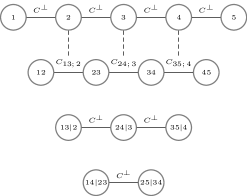
(a) Vine copula in Example 4.2.

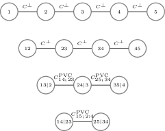
(b) PVC of Example 4.2.

Figure 2: The non-simplified D-vine copula given in Example 4.2 and its PVC. The influence of conditioning variables on the conditional copulas is indicated by dashed lines.

Lemma 4.2 (The PVC of Example 4.2)

Let $C_{1:5}$ be defined as in Example 4.2. Then

$$C^{\text{\tiny PVC}}_{12}=C^{\text{\tiny PVC}}_{23}=C^{\text{\tiny PVC}}_{34}=C^{\text{\tiny PVC}}_{45},\ \ C^{\text{\tiny PVC}}_{13;\kern 0.56001pt2}\ \!\! =\ \!\!C^{\text{\tiny PVC}}_{24;\kern 0.56001pt3}=C^{\text{\tiny PVC}}_{35;\kern 0.56001pt4},\ \ C^{\text{\tiny PVC}}_{14;\kern 0.56001pt2:3}=C^{\text{\tiny PVC}}_{25;\kern 0.56001pt3:4},$$

$$C^{\text{\tiny PVC}}_{12}\ =\ C^{\perp},$$

$$C^{\text{\tiny PVC}}_{13;\kern 0.56001pt2}\ =\ C^{\perp},$$

$$C^{\text{\tiny PVC}}_{14;\kern 0.56001pt2:3}(a,b)\ =\ C^{FGM_{2}}(a,b\ \!;1/9),\quad\forall(a,b)\in[0,1]^{2}$$

$$C^{\text{\tiny PVC}}_{15;\kern 0.56001pt2:4}\ \neq\ C^{\perp},$$

and

$$U^{\text{\tiny PVC}}_{1|2}=U_{1}\ =\ U_{1|2},$$

$$U^{\text{\tiny PVC}}_{1|2:3}=U_{1}\ \neq\ U_{1|2:3}=U_{1}[1+(1-U_{1})(1-2U_{2})(1-2U_{3})],$$

$$U^{\text{\tiny PVC}}_{1|2:4}=U_{1}[1+\theta(1-U_{1})(1-2U_{4})]\ \neq\ U_{1|2:4}=U_{1|2:3}.$$

Proof.

See Section A.4. $\blacksquare$

Lemma 4.2 demonstrates that $j$-th order partial copulas may not be independence copulas, although the corresponding conditional copulas are independence copulas. In particular, under the data generating process the edges of the third tree of $C_{1:5}$ are independence copulas. Neglecting the conditional copulas in the second tree and replacing them with first-order partial copulas induces spurious dependencies in the third tree of $C^{\text{\tiny PVC}}_{1:5}$. The introduced spurious dependence also carries over to the fourth tree where we have (conditional) independence in fact. Nevertheless, the PVC reproduces the bivariate margins of $C_{1:5}$ pretty well. It can be readily verified that $(C^{\text{\tiny PVC}}_{13},C^{\text{\tiny PVC}}_{14},C^{\text{\tiny PVC}}_{24},C^{\text{\tiny PVC}}_{25},C^{\text{\tiny PVC}}_{35})=(C_{13},C_{14},C_{24},C_{25},C_{35})$, i.e., except for $C^{\text{\tiny PVC}}_{15}$, all bivariate margins of $C^{\text{\tiny PVC}}_{1:5}$ match the bivariate margins of $C_{1:5}$ in Example 4.2. Moreover, the mutual information in the third and fourth tree are larger if higher-order partial copulas are used instead of the true conditional copulas. Thus, the spurious dependence in the third and fourth tree decreases the Kullback-Leibler divergence from $C_{1:5}$ and therefore acts as a countermeasure for the spurious (conditional) independence in the second tree. Lemma 4.2 also reveals that $U_{1|2:4}$ is a function of $U_{2}$ and $U_{3}$, i.e. the true conditional distribution function $F_{1|2:4}$ depends on $u_{2}$ and $u_{3}$. In contrast, $F^{\text{\tiny PVC}}_{1|2:4}$, the resulting model for $F_{1|2:4}$ which is implied by the PVC, depends only on $u_{4}$. That is, the implied conditional distribution function of the PVC depends on the conditioning variable which actually has no effect.

5 Approximations based on the partial vine copula

The specification and estimation of SVCs is commonly based on procedures that asymptotically minimize the Kullback-Leibler divergence (KLD) in a stepwise fashion. For instance, if a parametric vine copula model is used, the step-by-step ML estimator (Hobæk Haff [29, 25]), where one estimates tree after tree and sequentially minimizes the estimated KLD conditional on the estimates from the previous trees, is often employed in order to select and estimate the parametric pair-copula families of the vine. But also the non-parametric methods of Kauermann and Schellhase [9] and Nagler and Czado [20] proceed in a stepwise manner and asymptotically minimize the KLD of each pair-copula separately under appropriate conditions. In this section, we investigate the role of the PVC when it comes to approximating non-simplified vine copulas.

Let $C_{1:d}\in{\cal C}_{d}$ and $C^{\text{\tiny SVC}}_{1:d}\in{\cal C}^{\text{\tiny SVC}}_{d}$. The KLD of $C^{\text{\tiny SVC}}_{1:d}$ from the true copula $C_{1:d}$ is given by

$$D_{KL}(C_{1:d}||C^{\text{\tiny SVC}}_{1:d}) =\mathbb{E}\left[\log\frac{c_{1:d}(U_{1:d})}{c^{\text{\tiny SVC}}_{1:d}(U_{1:d})}\right],$$

where the expectation is taken w.r.t. the true distribution $C_{1:d}$. We now decompose the KLD into the Kullback-Leibler divergences related to each of the $d-1$ trees. For this purpose, let $j=1,\ldots,d-1$ and define

$$\mathbf{T}_{j} :=\left\{(C^{\text{\tiny SVC}}_{i,i+j;\kern 0.56001ptS_{ij}})_{i=1,\ldots,d-j}\colon C^{\text{\tiny SVC}}_{i,i+j;\kern 0.56001ptS_{ij}}\in{\cal C}_{2}\text{ for }1\leq i\leq d-j\right\},$$

so that $\mathbf{T}_{1:j}=\times_{k=1}^{j}\mathbf{T}_{k}$ represents all possible SVCs up to and including the $j$-th tree. Let ${{\cal T}}_{j}\in\mathbf{T}_{j},{{\cal T}}_{1:j-1}\in\mathbf{T}_{1:j-1}$. The KLD of the SVC associated with ${{\cal T}}_{1:d-1}$ is given by

$$D_{KL}(C_{1:d}||{{\cal T}}_{1:d-1}) =\sum_{j=1}^{d-1}D_{KL}^{(j)}({{{\cal T}_{j}}}({{\cal T}}_{1:j-1})),$$ (5.1)

where

$$D_{KL}^{(1)}({{\cal T}}_{1}({{\cal T}}_{1:0}))) :=D_{KL}^{(1)}({\cal T}_{1}):=\sum_{i=1}^{d-1}\mathbb{E}\left[\log\frac{c_{i,i+1}(U_{i},U_{i+1})}{c^{\text{\tiny SVC}}_{i,i+1}(U_{i},U_{i+1})}\right]$$

denotes the KLD related to the first tree, and for the remaining trees $j=2,\ldots,d-1$, the related KLD is

$$D_{KL}^{(j)}({{\cal T}_{j}}({{\cal T}}_{1:j-1})) :=\sum_{i=1}^{d-j}\mathbb{E}\left[\log\frac{c_{i,i+j;\kern 0.56001ptS_{ij}}(U_{i|S_{ij}},U_{i+j|S_{ij}}|U_{S_{ij}})}{c^{\text{\tiny SVC}}_{i,i+j;\kern 0.56001ptS_{ij}}(U^{\text{\tiny SVC}}_{i|S_{ij}},U^{\text{\tiny SVC}}_{i+j|S_{ij}})}\right].$$

For instance, if $d=3$, the KLD can be decomposed into the KLD related to the first tree $D_{KL}^{(1)}$ and to the second tree $D_{KL}^{(2)}$ as follows

$$D_{KL}(C_{1:3}||{\cal T}_{1:2}) =D_{KL}(C_{1:3}||({\cal T}_{1},{\cal T}_{2}))=D_{KL}^{(1)}({{\cal T}}_{1})+D_{KL}^{(2)}({{\cal T}}_{2}({{\cal T}}_{1}))$$

$$=\mathbb{E}\left[\log\frac{{c}_{12}(U_{1:2}){c}_{23}(U_{2:3})}{c^{\text{\tiny SVC}}_{12}(U_{1:2})c^{\text{\tiny SVC}}_{23}(U_{2:3})}\right]+\mathbb{E}\left[\log\frac{{c}_{13;\kern 0.56001pt2}\big{(}\partial_{2}{C}_{12}(U_{1:2}),\partial_{1}{C}_{23}(U_{2:3})|U_{2}\big{)}}{c^{\text{\tiny SVC}}_{13;\kern 0.56001pt2}\big{(}\partial_{2}C^{\text{\tiny SVC}}_{12}(U_{1:2}),\partial_{1}C^{\text{\tiny SVC}}_{23}(U_{2:3})\big{)}}\right].$$

Note that the KLD related to tree $j$ depends on the specified copulas in the lower trees because they determine at which values the copulas in tree $j$ are evaluated. The following theorem shows that, if one sequentially minimizes the KLD related to each tree, then the optimal SVC is the PVC.

Theorem 5.1 (Tree-by-tree KLD minimization using the PVC)

Let $C_{1:d}\in{\cal C}_{d}$ be the data generating copula and ${\cal T}^{\text{\tiny PVC}}_{j}:=(C^{\text{\tiny PVC}}_{i,i+j;\kern 0.56001ptS_{ij}})_{i=1,\ldots,d-j}$, so that ${\cal T}^{\text{\tiny PVC}}_{1:j}:=\times_{k=1}^{j}{\cal T}^{\text{\tiny PVC}}_{k}$ collects all copulas of the PVC up to and including the $j$-th tree. It holds that

$$\forall j=1,\ldots,d-1\colon\quad\operatorname*{\!\!\!\!\!\!\!\!\phantom{{}_{p}}\arg\min\phantom{{}_{p}}\!\!\!\!\!\!\!\!}_{{\cal T}_{j}\in\mathbf{T}_{j}}\quad\!D_{KL}^{(j)}({\cal T}_{j}({\cal T}^{\text{\tiny PVC}}_{1:j-1})) ={\cal T}^{\text{\tiny PVC}}_{j}.$$ (5.2)

Proof.

See Section A.5. $\blacksquare$

According to Theorem 5.1, if the true copulas are specified in the first tree, one should choose the first-order partial copulas in the second tree, the second-order partial copulas in the third tree etc. to minimize the KLD tree-by-tree. Theorem 5.1 also remains true if we replace ${\cal C}_{2}$ in the definition of $\mathbf{T}_{j}$ by the space of absolutely continuous bivariate cdfs. The PVC ensures that random variables in higher trees are uniformly distributed since the resulting random variables in higher trees are higher-order PPITs. If one uses a different approximation, such as the one used by Hobæk Haff et al. [13] and Stöber et al. [14], then the random variables in higher trees are not necessarily uniformly distributed and pseudo-copulas (Fermanian and Wegkamp [30]) can be used to further minimize the KLD. Stöber et al. [14] note in their appendix that if $C_{1:3}$ is a FGM copula and the copulas in the first tree are correctly specified, then the KLD from the true distribution has an extremum at $C^{\text{\tiny SVC}}_{13;\kern 0.56001pt2}=C^{\perp}=C^{\text{\tiny PVC}}_{13;\kern 0.56001pt2}$. If $C_{13;\kern 0.56001pt2}$ belongs to a parametric family of bivariate copulas whose parameter depends on $u_{2}$, then $C^{\text{\tiny PVC}}_{13;\kern 0.56001pt2}$ is in general not a member of the same copula family with a constant parameter, see Spanhel and Kurz [18]. Together with Theorem 5.1 it follows that the proposed simplified vine copula approximations of Hobæk Haff et al. [13] and Stöber et al. [14] can be improved if the first-order partial copula is chosen in the second tree, and not a copula of the same parametric family as the conditional copula but with a constant dependence parameter such that the KLD is minimized.

Besides its interpretation as generalization of the partial correlation matrix, the PVC can also be interpreted as the SVC that minimizes the KLD tree-by-tree. This sequential minimization neglects that the KLD related to a tree depends on the copulas that are specified in the former trees. For instance, if $d=3$, the KLD of the first tree $D_{KL}^{(1)}({\cal T}_{1})$ is minimized over the copulas $({C^{\text{\tiny SVC}}_{12},C^{\text{\tiny SVC}}_{23}})$ in the first tree ${\cal T}_{1}$, but the effect of the chosen copulas in the first tree ${\cal T}_{1}$ on the KLD related to the second tree $D_{KL}^{(2)}({{{\cal T}}_{2}({{\cal T}}_{1}))}$ is not taken into account. Therefore, we now analyze whether the PVC also globally minimizes the KLD. Note that specifying the wrong margins in the first tree ${\cal T}_{1}$, e.g., $(C^{\text{\tiny SVC}}_{12},C^{\text{\tiny SVC}}_{23})\neq(C_{12},C_{23})$, increases $D_{KL}^{(1)}({\cal T}_{1})$ in any case. Thus, without any further investigation, it is absolutely indeterminate whether the definite increase in $D_{KL}^{(1)}({\cal T}_{1})$ can be overcompensated by a possible decrease in $D_{KL}^{(2)}({\cal T}_{2}({\cal T}_{1}))$ if another approximation is chosen. The next theorem shows that the PVC is in general not the global minimizer of the KLD.

Theorem 5.2 (Global KLD minimization if $C_{1:d}\in{\cal C}^{\text{\tiny SVC}}_{d}$ or $C_{1:d}\in{\cal C}_{d}\backslash{\cal C}^{\text{\tiny SVC}}_{d}$)

If $C_{1:d}\in{\cal C}^{\text{\tiny SVC}}_{d}$, i.e., the simplifying assumption holds for $C_{1:d}$, then

$$\operatorname*{\!\!\!\!\!\!\!\!\phantom{{}_{p}}\arg\min\phantom{{}_{p}}\!\!\!\!\!\!\!\!}_{C^{\text{\tiny SVC}}_{1:d}\in{\cal C}^{\text{\tiny SVC}}_{d}}D_{KL}(C_{1:d}||C^{\text{\tiny SVC}}_{1:d}) =C^{\text{\tiny PVC}}_{1:d}.$$ (5.3)

If the simplifying assumption does not hold for $C_{1:d}$, then $C^{\text{\tiny PVC}}_{1:d}$ might not be a global minimum. That is, $\exists C_{1:d}\in{\cal C}_{d}\backslash{\cal C}^{\text{\tiny SVC}}_{d}$ such that

$$\operatorname*{\!\!\!\!\!\!\!\!\phantom{{}_{p}}\arg\min\phantom{{}_{p}}\!\!\!\!\!\!\!\!}_{C^{\text{\tiny SVC}}_{1:d}\in{\cal C}^{\text{\tiny SVC}}_{d}}D_{KL}(C_{1:d}||C^{\text{\tiny SVC}}_{1:d}) \neq C^{\text{\tiny PVC}}_{1:d},$$ (5.4)

and $\forall({\cal T}_{2},\ldots,{\cal T}_{d-1})\in\times_{k=2}^{d-1}\mathbf{T}_{k}$

$$\operatorname*{\!\!\!\!\!\!\!\!\phantom{{}_{p}}\arg\min\phantom{{}_{p}}\!\!\!\!\!\!\!\!}_{\tilde{\cal T}_{1:d-1}\in\mathbf{T}_{1:d-1}}D_{KL}(C_{1:d}||\tilde{{\cal T}}_{1:d-1}) \neq({\cal T}^{\text{\tiny PVC}}_{1},{\cal T}_{2},\ldots,{\cal T}_{d-1}).$$ (5.5)

Proof.

See Section A.6. $\blacksquare$

Theorem 5.2 states that, if the simplifying assumption does not hold, the KLD may not be minimized by choosing the true copulas in the first tree, first-order partial copulas in the second tree and higher-order partial copulas in the remaining trees (see (5.4)). It follows that, if the objective is the minimization of the KLD, it may not be optimal to specify the true copulas in the first tree, no matter what bivariate copulas are specified in the other trees (see (5.5)). This rather puzzling result can be explained by the fact that, if the simplifying assumption does not hold, then the approximation error of the implicitly modeled bivariate margins is not minimized (see Lemma 4.1). For instance, if $d=3$, a departure from the true copulas $(C_{12},C_{23})$ in the first tree increases the KLD related to the first tree, but it can decrease the KLD of the implicitly modeled margin $C^{\text{\tiny SVC}}_{13}$ from $C_{13}$. As a result, the increase in $D_{KL}^{(1)}$ can be overcompensated by a larger decrease in $D_{KL}^{(2)}$, so that the KLD can be decreased.

Theorem 5.2 does not imply that the PVC never minimizes the KLD from the true copula. For instance, if $d=3$ and if $C^{\text{\tiny PVC}}_{13;\kern 0.56001pt2}=C^{\perp}$, then $D_{KL}(C_{1:3}||C^{\text{\tiny PVC}}_{1:3})$ is an extremum, which directly follows from equation (5.2) since

$$\operatorname*{\!\!\!\!\!\!\!\!\phantom{{}_{p}}\arg\min\phantom{{}_{p}}\!\!\!\!\!\!\!\!}_{{\cal T}_{1}\in\mathbf{T}_{1}}\ D_{KL}(C_{1:3}||({\cal T}_{1},(C^{\perp}))) =\ \ \operatorname*{\!\!\!\!\!\!\!\!\phantom{{}_{p}}\arg\min\phantom{{}_{p}}\!\!\!\!\!\!\!\!}_{{\cal T}_{1}\in\mathbf{T}_{1}}\ D_{KL}^{(1)}({{{{\cal T}}_{1}}}).$$

It is an open problem whether and when the PVC can be the global minimizer of the KLD. Unfortunately, the simplified vine copula approximation that globally minimizes the KLD is not tractable. However, if the simplified vine copula approximation that minimizes the KLD does not specify the true copulas in the first tree, the random variables in the higher tree are not CPITs. Thus, it is not guaranteed that these random variables are uniformly distributed and we could further decrease the KLD by assigning pseudo-copulas (Fermanian and Wegkamp [30]) to the edges in the higher trees. It can be easily shown that the resulting best approximation is then a pseudo-copula. Consequently, the best approximation satisfying the simplifying assumption is in general not an SVC but a simplified vine pseudo-copula if one considers the space of regular vines where each edge corresponds to a bivariate cdf.

While the PVC may not be the best approximation in the space of SVCs, it is the best feasible SVC approximation in practical applications. That is because the stepwise specification and estimation of an SVC is also feasible for (very) large dimensions which is not true for a joint specification and estimation. For instance, if all pair-copula families of a parametric vine copula are chosen simultaneously and the selection is done by means of information criteria, we have to estimate $K^{d(d-1)/2}$ different models, where $d$ is the dimension and $K$ the number of possible pair-copula families that can be assigned to each edge. On the contrary, a stepwise procedure only requires the estimation of $Kd(d-1)/2$ models. To illustrate the computational burden, consider the R-package VineCopula [31] where $K=40$. For this number of pair-copula families, a joint specification requires the estimation of 64,000 ($d=3$) or more than four billion ($d=4$) models whereas only 120 ($d=3$) or 240 ($d=4$) models are needed for a stepwise specification. For many non-parametric estimation approaches (kernels [20], empirical distributions [32]), only the sequential estimation of an SVC is possible. The only exception is the spline-based approach of Kauermann and Schellhase [9]. However, due to the large number of parameters and the resulting computational burden, a joint estimation is only feasible for $d\leq 5$ [33].

6 Convergence to the partial vine copula

If the data generating process satisfies the simplifying assumption, consistent stepwise procedures for the specification and estimation of parametric and non-parametric simplified vine copula models asymptotically minimize the KLD from the true copula. Theorem 5.1 implies that this is not true in general if the data generating process does not satisfy the simplifying assumption. An implication of this result for the application of SVCs is pointed out in the next corollary.

Corollary 6.1

Denote the sample size by $N$. Let $C_{1:d}\in{\cal C}_{d}$ be the data generating copula and $C^{\text{\tiny SVC}}_{1:d}(\theta)\in{\cal C}^{\text{\tiny SVC}}_{d},\theta\in\Theta$, be a parametric SVC so that $\exists_{1}\theta_{\text{\tiny PVC}}\in\Theta:C^{\text{\tiny SVC}}_{1:d}(\theta_{\text{\tiny PVC}})=C^{\text{\tiny PVC}}_{1:d}$. The pseudo-true parameters which minimize the KLD from the true distribution are assumed to exist (see White [34] for sufficient conditions) and denoted by

$$\theta^{\star} =\ \ \operatorname*{\!\!\!\!\!\!\!\!\phantom{{}_{p}}\arg\min\phantom{{}_{p}}\!\!\!\!\!\!\!\!}_{\theta\in\Theta}\ \ D_{KL}(C_{1:d}||C^{\text{\tiny SVC}}_{1:d}(\theta)).$$

Let $\hat{\theta}_{S}$ denote the (semi-parametric) step-by-step ML estimator and $\hat{\theta}_{J}$ denote the (semi-parametric) joint ML estimator defined in Hobæk Haff [29, 25]. Under regularity conditions (e.g., Condition 1 and Condition 2 in [35]) and for $N\to\infty$, it holds that:

1. $\hat{\theta}^{S}\stackrel{{\scriptstyle p}}{{\to}}\theta^{\text{\tiny PVC}}.$

2. $\hat{\theta}^{J}\stackrel{{\scriptstyle p}}{{\to}}{\theta}^{\star}.$

3. $\exists C_{1:d}\in{\cal C}_{d}\backslash{\cal C}^{\text{\tiny SVC}}_{d}$ such that $\hat{\theta}^{S}\not\stackrel{{\scriptstyle p}}{{\to}}\theta^{\star}.$

Proof.

See Section A.8. $\blacksquare$

Corollary 6.1 shows that the step-by-step and joint ML estimator may not converge to the same limit (in probability) if the simplifying assumption does not hold for the data generating vine copula. For this reason, we investigate in the following the difference between the step-by-step and joint ML estimator in finite samples. Note that the convergence of kernel-density estimators to the PVC has been recently established by Nagler and Czado [20]. However, in this case, only a sequential estimation of a simplified vine copula is possible and thus the best feasible approximation in the space of simplified vine copulas is given by the PVC.

6.1 Difference between step-by-step and joint ML estimates

We compare the step-by-step and the joint ML estimator under the assumption that the pair-copula families of the PVC are specified for the parametric vine copula model. For this purpose, we simulate data from two three-dimensional copulas $C_{1:3}$ with sample sizes $N=\ 500,2500,25000$, perform a step-by-step and joint ML estimation, and repeat this 1000 times. For ease of exposition and because the qualitative results are not different, we consider copulas where $C_{12}=C_{23}$ and only present the estimates for $(\theta_{12},\theta_{13;2})$.

Example 6.1 (PVC of the Frank copula)

Let $C^{\text{Fr}}(\theta)$ denote the bivariate Frank copula with dependence parameter $\theta$ and ${C}^{\text{P-Fr}}(\theta)$ be the partial Frank copula [18] with dependence parameter $\theta$. Let $C_{1:3}$ be the true copula with $(C_{12},C_{23},C_{13;\kern 0.56001pt2})=(C^{\text{Fr}}(5.74),C^{\text{Fr}}(5.74),{C}^{\text{P-Fr}}(5.74))$, i.e., $C_{1:3}=C^{\text{\tiny PVC}}_{1:3}$, and $C^{\text{\tiny SVC}}_{1:3}(\theta)=(C^{\text{Fr}}(\theta_{12}),C^{\text{Fr}}(\theta_{23}),{C}^{\text{P-Fr}}(\theta_{13;2}))$ be the parametric SVC that is fitted to data generated from $C_{1:3}$.

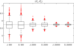
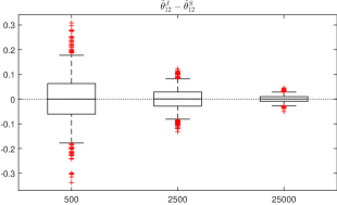
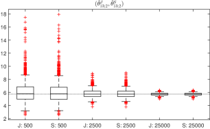
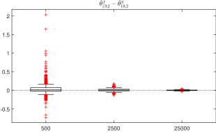
Figure 3: Box plots of joint (J) and sequential (S) ML estimates and their difference for sample sizes $N=500,2500,25000$, if the data is generated from $C_{1:3}$ in Example 6.1 and the pair-copula families of the SVC are given by the corresponding PVC. The dotted line indicates the pseudo-true parameter and zero, respectively. The end of the whiskers is 0.953 times the inter-quartile range, corresponding to approximately 95% coverage if the data is generated by a normal distribution.

Example 6.1 presents a data generating process which satisfies the simplifying assumption, implying $\theta^{\text{\tiny PVC}}=\theta^{\star}$. It is the PVC of the three-dimensional Frank copula with Kendall’s $\tau$ approximately equal to 0.5. Figure 3 shows the corresponding box plots of joint and step-by-step ML estimates and their difference. The left panel confirms the results of Hobæk Haff [29, 25]. Although the joint ML estimator is more efficient, the loss in efficiency for the step-by-step ML estimator is negligible and both estimators converge to the true parameter value. Moreover, the right panel of Figure 3 shows that the difference between joint and step-by-step ML estimates is never statistically significant at a 5% level. Since the computational time for a step-by-step ML estimation is much lower than for a joint ML estimation [29], the step-by-step ML estimator is very attractive for estimating high-dimensional vine copulas that satisfy the simplifying assumption. Moreover, the step-by-step ML estimator is then inherently suited for selecting the pair-copula families in a stepwise manner. However, if the simplifying assumption does not hold for the data generating vine copula, the step-by-step and joint ML estimator can converge to different limits (Corollary 6.1), as the next example demonstrates.

Example 6.2 (Frank copula)

Let $C_{1:3}$ be the Frank copula with dependence parameter $\theta=5.74$, i.e., $C_{1:3}\neq C^{\text{\tiny PVC}}_{1:3}$, and $C^{\text{\tiny SVC}}_{1:3}=(C^{\text{Fr}}(\theta_{12}),C^{\text{Fr}}(\theta_{23}),{C}^{\text{P-Fr}}(\theta_{13;2}))$ be the parametric SVC that is fitted to data generated from $C_{1:3}$.

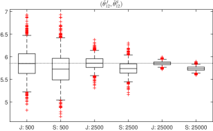
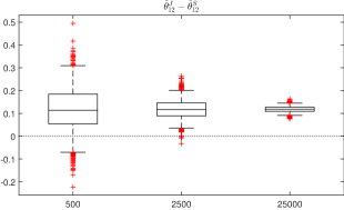
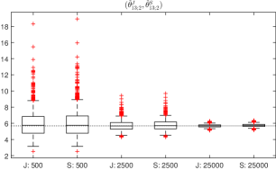
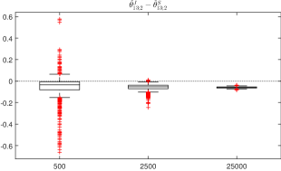
Figure 4: Box plots of joint (J) and sequential (S) ML estimates and their difference for sample sizes $N=500,2500,25000$, if the data is generated from $C_{1:3}$ in Example 6.2 and the pair-copula families of the SVC are given by the corresponding PVC. The dotted line indicates the pseudo-true parameter and zero, respectively. The end of the whiskers is 0.953 times the inter-quartile range, corresponding to approximately 95% coverage if the data is generated by a normal distribution.

Example 6.2 is identical to Example 6.1, with the only difference that the conditional copula is varying in such a way that the resulting three-dimensional copula is a Frank copula. Although the Frank copula does not satisfy the simplifying assumption, it is pretty close to a copula for which the simplifying assumption holds, because the variation in the conditional copula is strongly limited for Archimedean copulas (Mesfioui and Quessy [36]). Nevertheless, the right panel of Figure 4 shows that the step-by-step and joint ML estimates for $\theta_{12}$ are significantly different at the 5% level if the sample size is 2500 observations. The difference between step-by-step and joint ML estimates for $\theta_{13;\kern 0.56001pt2}$ is less pronounced, but also highly significant for sample sizes with 2500 observations or more. Thus, only in Example 6.1 the step-by-step ML estimator is a consistent estimator of a simplified vine copula model that minimizes the KLD from the underlying copula, whereas the joint ML estimator is a consistent minimizer in both examples. A third example where the distance between the data generating copula and the PVC and thus the difference between the step-by-step and joint ML estimates is more pronounced is given in Section A.9.

7 Conclusion

We introduced the partial vine copula (PVC) which is a particular simplified vine copula that coincides with the data generating copula if the simplifying assumption holds. The PVC can be regarded as a generalization of the partial correlation matrix where partial correlations are replaced by $j$-th order partial copulas. Consequently, it provides a new dependence measure of a $d$-dimensional distribution in terms of $d(d-1)/2$ bivariate unconditional copulas. While a higher-order partial copula of the PVC is related to the partial copula, it does not suffer from the curse of dimensionality and can be estimated for high-dimensional data [20]. We analyzed to what extent the dependence structure of the underlying distribution is reproduced by the PVC. In particular, we showed that a pair of random variables may be considered as conditionally (in)dependent according to the PVC although this is not the case for the data generating process.

We also revealed the importance of the PVC for the modeling of high-dimensional distributions by means of simplified vine copulas (SVCs). Up to now, the estimation of SVCs has almost always been based on the assumption that the data generating process satisfies the simplifying assumption. Moreover, the implications that follow if the simplifying assumption is not true have not been investigated. We showed that the PVC is the SVC approximation that minimizes the Kullback-Leibler divergence in a stepwise fashion. Since almost all estimators of SVCs proceed sequentially, it follows that, under regularity conditions, many estimators of SVCs converge to the PVC also if the simplifying assumption does not hold. However, we also proved that the PVC may not minimize the Kullback-Leibler divergence from the true copula and thus may not be the best SVC approximation in theory. Nevertheless, due to the prohibitive computational burden or simply because only a stepwise model specification and estimation is possible, the PVC is the best feasible SVC approximation in practice.

The analysis in this paper showed the relative optimality of the PVC when it comes to approximating multivariate distributions by SVCs. Obviously, it is easy to construct (theoretical) examples where the PVC does not provide a good approximation in absolute terms. But such examples do not provide any information about the appropriateness of the simplifying assumption in practice. To investigate whether the simplifying assumption is true and the PVC is a good approximation in applications, one can use Lemma 3.1 to develop tests for the simplifying assumption, see Kurz and Spanhel [21]. Moreover, even in cases where the simplifying assumption is strongly violated, an estimator of the PVC can yield an approximation that is superior to competing approaches. Recently, it has been demonstrated in Nagler and Czado [20] that the structure of the PVC can be used to obtain a constrained kernel-density estimator that can be much closer to the data generating process than the classical unconstrained kernel-density estimator, even if the distance between the PVC and the data generating copula is large.

Appendix

A.1 Proof of Lemma 3.1

$U^{\text{\tiny PVC}}_{k|S_{ij}}=U_{k|S_{ij}}\ (a.s.)\Rightarrow U^{\text{\tiny PVC}}_{k|S_{ij}}\perp U_{S_{ij}}$ is true because $U_{k|S_{ij}}$ is a CPIT. For the converse, let Let $A:=\times_{k=i+1}^{i+j-1}[0,u_{k}]$ and consider

$$P(U^{\text{\tiny PVC}}_{k|S_{ij}}\leq a,U_{S_{ij}}\leq u_{S_{ij}}) =\int_{A}F_{k|S_{ij}}\big{(}(F^{\text{\tiny PVC}}_{k|S_{ij}})^{-1}(a|t_{S_{ij}})|t_{S_{ij}}\big{)}\text{d}C_{{S_{ij}}}(t_{S_{ij}}).$$ (A.1)

Since $U^{\text{\tiny PVC}}_{k|S_{ij}}\sim U(0,1)$ it follows that if $U^{\text{\tiny PVC}}_{k|S_{ij}}\perp U_{S_{ij}}$ then $P(U^{\text{\tiny PVC}}_{k|S_{ij}}\leq a,U_{S_{ij}}\leq u_{S_{ij}})=aC_{{S_{ij}}}(u_{S_{ij}})$ for all $(a,u_{S_{ij}})\in[0,1]^{j}$. This implies that

$$P(U^{\text{\tiny PVC}}_{k|S_{ij}}\leq a,U_{S_{ij}}\leq u_{S_{ij}}) =\int_{A}a\ \!\text{d}C_{{S_{ij}}}(t_{S_{ij}})$$

equals the right hand side of (A.1) for all $(a,u_{S_{ij}})\in[0,1]^{j}$. It follows that the integrands must be identical (a.s.) as well and $F_{k|S_{ij}}(F^{\text{\tiny PVC}}_{k|S_{ij}})^{-1}(a|t_{S_{ij}})=a$ for all $a\in[0,1]$ and almost every $(u_{S_{ij}})\in[0,1]^{j}$. Thus $F_{k|S_{ij}}=F^{\text{\tiny PVC}}_{k|S_{ij}}$ (a.s.) which is equivalent to $U^{\text{\tiny PVC}}_{k|S_{ij}}=U_{k|S_{ij}}\ (a.s.)$.

A.2 Proof of Lemma 4.1

Let ${C}^{\star}_{1:3}\in{\cal C}^{\text{\tiny SVC}}_{3}$ be the SVC given in Example 4.1. We define $C_{1:d}$ as follows. Let $C_{1,d-1;\kern 0.56001pt2:d-2}=C^{\star}_{12},C_{2,d;\kern 0.56001pt3:d-1}=C^{\star}_{23}$, $C_{1,d;\kern 0.56001pt2:d-1}={D}^{\star}_{1,3;\kern 0.56001pt2}$, where $D^{\star}_{1,3;\kern 0.56001pt2}$ is the corresponding conditional copula in Example 4.1 and $C_{i,i+j;\kern 0.56001ptS_{ij}}=E_{k,l}\in{\cal C}_{2},(k,l)\in{\cal I}_{1}^{d}$ means that $C_{i,i+j;\kern 0.56001ptS_{ij}}(a,b|u_{S_{ij}})=E_{k,l}(a,b)$ for all $(a,b,u_{S_{ij}})\in[0,1]^{j+1}$. Moreover, let $C_{i,i+j;\kern 0.56001ptS_{ij}}=C^{\perp}$ for $(i,j)\in{\cal I}_{1}^{d}\backslash\{(1,d-2),(2,d-2),(1,d-1)\}$. The conclusion now follows from Example 4.1.

A.3 Proof of Theorem 4.1

W.l.o.g. assume that the margins of $X_{1:d}$ are uniform. Let $C^{FGM_{3}}(u_{1:3};\theta)=\prod_{i=1}^{3}u_{i}+\theta\prod_{i=1}^{3}u_{i}(1-u_{i}),|\theta|\leq 1$, be the three-dimensional FGM copula, $d\geq 4$, and $(i,j)\in{\cal I}_{1}^{d}$. It is obvious that $C_{i,i+2;\kern 0.56001pti+1}=C^{\perp}\Rightarrow C^{\text{\tiny PVC}}_{i,i+2;\kern 0.56001pti+1}=C^{\perp}$ is true. Let $J\in\{2,\ldots,d-2\}$ be fixed. Assume that $C_{1:d}$ has the following D-vine copula representation of the non-simplified form

$$C_{1,1+J;\kern 0.56001pt2:J} =\partial_{3}C^{FGM_{3}}(u_{1},u_{1+J},u_{2};1)$$

$$C_{2,2+J;\kern 0.56001pt3:J+1} =\partial_{3}C^{FGM_{3}}(u_{2},u_{2+J},u_{1+J};1)$$

and $C_{i,i+j;\kern 0.56001ptS_{i,j}}=C^{\perp}$ for all other $(i,j)\in{\cal I}_{1}^{d}$. Using the same arguments as in the proof of Lemma 4.2 we obtain

$$C^{\text{\tiny PVC}}_{i,i+J;\kern 0.56001pti+1:J-1} =C^{\perp},\quad i=1,2,$$

$$C^{\text{\tiny PVC}}_{1,2+J;\kern 0.56001pt2:J+1} =C^{FGM_{2}}(1/9).$$

This proves that $C_{i,i+2;\kern 0.56001pti+1}=C^{\perp}\Leftarrow C^{\text{\tiny PVC}}_{i,i+2;\kern 0.56001pti+1}=C^{\perp}$ is not true in general and that, for $j\geq 3$, neither the statement $C_{i,i+j;\kern 0.56001ptS_{ij}}=C^{\perp}\Rightarrow C^{\text{\tiny PVC}}_{i,i+j;\kern 0.56001ptS_{ij}}=C^{\perp}$ nor the statement $C_{i,i+j;\kern 0.56001ptS_{ij}}=C^{\perp}\Leftarrow C^{\text{\tiny PVC}}_{i,i+j;\kern 0.56001ptS_{ij}}=C^{\perp}$ is true in general.

A.4 Proof of Lemma 4.2

We show a more general result and set $C_{i,i+2;\kern 0.56001pti+1}(u_{i},u_{i+2}|u_{i+1})=C^{FGM_{2}}(u_{i},u_{i+2};g(u_{i+1}))$ in (4.3) where $g\colon[0,1]\to[-1,1]$ is a non-constant measurable function such that

$$\forall u\in[0.5,1]\colon g(0.5+u)=-g(0.5-u).$$ (A.2)

For $i=1,2,3,$ the copula in the second tree of the PVC is given by

$$C^{\text{\tiny PVC}}_{i,i+2;\kern 0.56001pti+1}(a,b) =\mathbb{P}(U_{i|i+1}\leq a,U_{i+2|i+1}\leq b)=\int_{[0,1]}C_{i,i+2;\kern 0.56001pti+1}(a,b|u_{i+1})\text{d}u_{i+1}$$

$$\ \ \stackrel{{\scriptstyle\text{\tiny\makebox[0.0pt]{\eqref{uncondfgm}}}}}{{=}}\ \ ab\big{(}1+(1-a)(1-b)\int_{[0,1]}g(u_{i+1})\text{d}u_{i+1}\big{)}\ \ \stackrel{{\scriptstyle\text{\tiny\makebox[0.0pt]{\eqref{gsym}}}}}{{=}}\ \ ab,$$ (A.3)

which is the independence copula. For $i=1,2,k=i,i+3$, the true CPIT of $U_{k}$ w.r.t. $U_{i+1:i+2}$ is a function of $U_{i+1:i+2}$ because

$$U_{i|i+1:i+2} =U_{i}[1+g(U_{i+1})(1-U_{i})(1-2U_{i+2})],$$ (A.4)

$$U_{i+3|i+1:i+2} =U_{i+3}[1+g(U_{i+2})(1-U_{i+3})(1-2U_{i+1})].$$ (A.5)

However, for $i=1,2,k=i,i+3$, the PPIT of $U_{k}$ w.r.t. $U_{i+1:i+2}$ is not a function of $U_{i+1:i+2}$ because

$$U^{\text{\tiny PVC}}_{i|i+1:i+2} =F^{\text{\tiny PVC}}_{i|i+1:i+2}(U_{i}|U_{i+1:i+2})=F_{U_{i|i+1}|U_{i+2|i+1}}(U_{i|i+1}|U_{i+2|i+1})$$

$$=\partial_{2}C_{i,i+2;\kern 0.56001pti+1}^{\text{\tiny PVC}}(U_{i|i+1},U_{i+2|i+1})\ \ \stackrel{{\scriptstyle\text{\tiny\makebox[0.0pt]{\eqref{eqPartial}}}}}{{=}}\ \ U_{i|i+1}\ \ \stackrel{{\scriptstyle\text{\tiny\makebox[0.0pt]{\eqref{eqCPIT}}}}}{{=}}\ \ U_{i},$$ (A.6)

and, by symmetry,

$$U^{\text{\tiny PVC}}_{i+3|i+1:i+2} =U_{i+3}.$$ (A.7)

For $i=1,2$, the joint distribution of these first-order PPITs is a copula in the third tree of the PVC which is given by

$$C^{\text{\tiny PVC}}_{i,i+3;\kern 0.56001pti+1:i+2}(a,b) =\mathbb{P}(U^{\text{\tiny PVC}}_{i|i+1:i+2}\leq a,U^{\text{\tiny PVC}}_{i+3|i+1:i+2}\leq b)\quad\ \ \stackrel{{\scriptstyle\text{\tiny\makebox[0.0pt]{\eqref{eqPCPIT1_1},\eqref{eqPCPIT1_2}}}}}{{=}}\quad\ \ \mathbb{P}(U_{i}\leq a,U_{i+3}\leq b)=C_{i,i+3}(a,b)$$ (A.8)

$$\stackrel{{\scriptstyle\text{\tiny\makebox[0.0pt]{\eqref{uncondfgm2}}}}}{{=}}\quad\int_{[0,1]^{2}}F_{i|i+1:i+2}(a|u_{i+1:i+2})F_{i+3|i+1:i+2}(b|u_{i+1:i+2})\text{d}u_{i+1:i+2}$$

$$\stackrel{{\scriptstyle\text{\tiny\makebox[0.0pt]{\eqref{eqCPIT1_1},\eqref{eqCPIT1_2}}}}}{{=}}\quad\ \ ab[1+(1-a)(1-b)\int_{[0,1]}g(u_{i+1})(1-2u_{i+1})\text{d}u_{i+1}\int_{[0,1]}g(u_{i+2})(1-2u_{i+2})\text{d}u_{i+2}]$$

$$=ab[1+\theta(1-a)(1-b)]=C^{FGM_{2}}(\theta),$$

where $\theta:=4(\int_{[0,1]}ug(u)\text{d}u)^{2}>0$, by the properties of $g$. Thus, a copula in the third tree of the PVC is a bivariate FGM copula whereas the true conditional copula is the independence copula.

The CPITs of $U_{1}$ or $U_{5}$ w.r.t. $U_{2:4}$ are given by

$$U_{1|2:4} =F_{1|2:4}(U_{1}|U_{2:4})=\partial_{2}C_{14;\kern 0.56001pt2:3}(U_{1|2:3},U_{4|2:3}|U_{2:3})\ \ \stackrel{{\scriptstyle\text{\tiny\makebox[0.0pt]{\eqref{uncondfgm2}}}}}{{=}}\ \ U_{1|2:3}$$

$$\stackrel{{\scriptstyle\text{\tiny\makebox[0.0pt]{\eqref{eqCPIT1_1}}}}}{{=}}\ \ U_{1}[1+g(U_{2})(1-U_{1})(1-2U_{3})],$$ (A.9)

$$U_{5|2:4} =\ \ U_{5}[1+g(U_{4})(1-U_{5})(1-2U_{3})],$$ (A.10)

whereas the corresponding second-order PPITs are given by

$$U^{\text{\tiny PVC}}_{1|2:4} =F^{\text{\tiny PVC}}_{1|2:4}(U_{1}|U_{2:4})=F_{U_{1|2:3}^{\text{\tiny PVC}}|U_{4|2:3}^{\text{\tiny PVC}}}(U_{1|2:3}^{\text{\tiny PVC}}|U_{4|2:3}^{\text{\tiny PVC}})\quad\ \ \stackrel{{\scriptstyle\text{\tiny\makebox[0.0pt]{\eqref{eqPCPIT1_1},\eqref{eqPCPIT1_2}}}}}{{=}}\quad\ \ F_{U_{1}|U_{4}}(U_{1}|U_{4})$$

$$=U_{1|4}=\partial_{2}C_{14}(U_{1},U_{4})\quad\stackrel{{\scriptstyle\text{\tiny\makebox[0.0pt]{\eqref{uncondmargfgm}}}}}{{=}}\quad U_{1}[1+\theta(1-U_{1})(1-2U_{4})],$$ (A.11)

$$U_{5|2:4}^{\text{\tiny PVC}} =U_{5}[1+\theta(1-U_{5})(1-2U_{2})].$$ (A.12)

For the copula in the fourth tree of the PVC it holds

$$C^{\text{\tiny PVC}}_{15;\kern 0.56001pt2:4}(a,b) =\mathbb{P}(U^{\text{\tiny PVC}}_{1|2:4}\leq a,U^{\text{\tiny PVC}}_{5|2:4}\leq b)\quad\;\stackrel{{\scriptstyle\text{\tiny\makebox[0.0pt]{\eqref{eqPCPIT2_1},\eqref{eqPCPIT2_2}}}}}{{=}}\quad\;\mathbb{P}(U_{1|4}\leq a,U_{5|2}\leq b)=\mathbb{P}(U_{1}\leq F_{1|4}^{-1}(a|U_{4}),U_{5}\leq F_{5|2}^{-1}(b|U_{2}))$$

$$=\int_{[0,1]^{3}}F_{15|2:4}(F_{1|4}^{-1}(a|u_{4}),F_{5|2}^{-1}(b|u_{2})|u_{2:4})c_{2:4}(u_{2:4})\text{d}u_{2:4}$$

$$=\int_{[0,1]^{3}}C_{15;\kern 0.56001pt2:4}(F_{1|2:4}(F_{1|4}^{-1}(a|u_{4})|u_{2:4}),F_{5|2:4}(F_{5|2}^{-1}(b|u_{2})|u_{2:4})|u_{2:4})c_{2:4}(u_{2:4})\text{d}u_{2:4}$$

$$\stackrel{{\scriptstyle\text{\tiny\makebox[0.0pt]{\eqref{uncondfgm3}}}}}{{=}}\int_{[0,1]^{3}}F_{1|2:4}(F_{1|4}^{-1}(a|u_{4})|u_{2:4})F_{5|2:4}(F_{5|2}^{-1}(b|u_{2})|u_{2:4})c_{2:4}(u_{2:4})\text{d}u_{2:4}$$

$$\stackrel{{\scriptstyle\text{\tiny\makebox[0.0pt]{\eqref{eqCPIT2_1},\eqref{eqCPIT2_2}}}}}{{=}}\quad\int_{[0,1]^{3}}F_{1|2:3}(F_{1|4}^{-1}(a|u_{4})|u_{2:3})F_{5|3:4}(F_{5|2}^{-1}(b|u_{2})|u_{3:4})c_{2:4}(u_{2:4})\text{d}u_{2:4}$$

$$\stackrel{{\scriptstyle\text{\tiny\makebox[0.0pt]{\eqref{eqCPIT1_1},\eqref{eqCPIT1_2}}}}}{{=}}\quad\int_{[0,1]^{3}}F_{1|4}^{-1}(a|u_{4})[1+g(u_{2})(1-F_{1|4}^{-1}(a|u_{4}))(1-2u_{3})]$$

$$\qquad\times F_{5|2}^{-1}(b|u_{2})[1+g(u_{4})(1-F_{5|2}^{-1}(b|u_{2}))(1-2u_{3})]\times[1+g(u_{3})(1-2u_{2})(1-2u_{4})]\text{d}u_{2:4}$$

$$=\int_{[0,1]^{2}}F_{1|4}^{-1}(a|u_{4})F_{5|2}^{-1}(b|u_{2})\left[1+\int_{[0,1]}(1-2u_{3})^{2}\text{d}u_{3}(1-F_{1|4}^{-1}(a|u_{4}))(1-F_{5|2}^{-1}(b|u_{2}))g(u_{4})g(u_{2})\right.$$

$$\qquad+\int_{[0,1]}(1-2u_{3})g(u_{3})\text{d}u_{3}(1-F_{5|2}^{-1}(b|u_{2}))(1-2u_{2})(1-2u_{4})g(u_{4})$$

$$\qquad+\left.\int_{[0,1]}(1-2u_{3})g(u_{3})\text{d}u_{3}(1-F_{1|4}^{-1}(a|u_{4}))(1-2u_{4})(1-2u_{2})g(u_{2})\right]\text{d}u_{2}\text{d}u_{4},$$

where we used that $$\int_{[0,1]}(1-2u_{3})\text{d}u_{3}=0 \int_{[0,1]}g(u_{3})\text{d}u_{3}\stackrel{{\scriptstyle\text{\tiny\makebox[0.0pt]{\eqref{gsym}}}}}{{=}}0 \int_{[0,1]}(1-2u_{3})^{2}g(u_{3})\text{d}u_{3}\stackrel{{\scriptstyle\text{\tiny\makebox[0.0pt]{\eqref{gsym}}}}}{{=}}0 \gamma:=-2\int_{[0,1]}ug(u)\text{d}u$$, and . By setting we can write the copula function as

$$C^{\text{\tiny PVC}}_{15;\kern 0.56001pt2:4}(a,b) =\int_{[0,1]^{2}}F_{1|4}^{-1}(a|u_{4})F_{5|2}^{-1}(b|u_{2})\left[1+\frac{1}{3}(1-F_{1|4}^{-1}(a|u_{4}))(1-F_{5|2}^{-1}(b|u_{2}))g(u_{4})g(u_{2})\right.$$

$$\qquad+\gamma(1-F_{5|2}^{-1}(b|u_{2}))(1-2u_{2})(1-2u_{4})g(u_{4})$$

$$\qquad+\left.\gamma(1-F_{1|4}^{-1}(a|u_{4}))(1-2u_{4})(1-2u_{2})g(u_{2})\right]\text{d}u_{2}\text{d}u_{4}$$

$$=\left(\int_{0}^{1}F_{1|4}^{-1}(a|u_{4})\text{d}u_{4}\right)\left(\int_{0}^{1}F_{5|2}^{-1}(b|u_{2})\text{d}u_{2}\right)$$

$$\qquad+\gamma\left(\int_{0}^{1}(1-2u_{2})(F_{5|2}^{-1}(b|u_{2})-(F_{5|2}^{-1}(b|u_{2}))^{2})\text{d}u_{2}\right)\left(\int_{0}^{1}(1-2u_{4})g(u_{4})F_{1|4}^{-1}(a|u_{4})\text{d}u_{4}\right)$$

$$\qquad+\gamma\left(\int_{0}^{1}(1-2u_{4})(F_{1|4}^{-1}(a|u_{4})-(F_{1|4}^{-1}(a|u_{4}))^{2})\text{d}u_{4}\right)\left(\int_{0}^{1}(1-2u_{2})g(u_{2})F_{5|2}^{-1}(b|u_{2})\text{d}u_{2}\right)$$

$$\qquad+\frac{1}{3}\left(\int_{0}^{1}g(u_{4})(F_{1|4}^{-1}(a|u_{4})-(F_{1|4}^{-1}(a|u_{4}))^{2})\text{d}u_{4}\right)\left(\int_{0}^{1}g(u_{2})(F_{5|2}^{-1}(b|u_{2})-(F_{5|2}^{-1}(b|u_{2}))^{2})\text{d}u_{2}\right)$$

If $(U,V)\sim C^{FGM_{2}}(\theta)$, the quantile function is given by (cf. Remillard [37])

$$F^{-1}_{U|V}(u|v) =\frac{1+h(v)-\sqrt{(1+h(v))^{2}-4h(v)u}}{2h(v)},$$

with $$h(v):=\theta(1-2v)$$, which implies

$$\frac{\partial}{\partial u}F_{U|V}^{-1}(u|v) =\frac{1}{\sqrt{(1+h(v))^{2}-4h(v)u}}=:G(u,v),$$ (A.13)

and

$$\frac{\partial}{\partial u}(F^{-1}_{U|V}(u|v))^{2} =\frac{1}{h(v)}\left[(1+h(v))G(u,v)-1\right].$$ (A.14)

For the density of the copula in the fourth tree of the PVC it follows

$$c^{\text{\tiny PVC}}_{15;\kern 0.56001pt2:4}(a,b) =\frac{\partial^{2}}{\partial a\partial b}C^{\text{\tiny PVC}}_{15;\kern 0.56001pt2:4}(a,b)$$

$$\stackrel{{\scriptstyle\text{\tiny\makebox[0.0pt]{\eqref{eqFGMderiv},\eqref{eqFGM2deriv}}}}}{{=}}\quad\;\left(\int_{0}^{1}G(a,u_{4})\text{d}u_{4}\right)\left(\int_{0}^{1}G(b,u_{2})\text{d}u_{2}\right)$$

$$\qquad+\frac{1}{\gamma}\left(1-\int_{0}^{1}G(b,u_{2})\text{d}u_{2}\right)\left(\int_{0}^{1}(1-2u_{4})g(u_{4})G(a,u_{4})\text{d}u_{4}\right)$$

$$\qquad+\frac{1}{\gamma}\left(1-\int_{0}^{1}G(a,u_{4})\text{d}u_{4}\right)\left(\int_{0}^{1}(1-2u_{2})g(u_{2})G(b,u_{2})\text{d}u_{2}\right)$$

$$\qquad+\frac{1}{3}\left(\int_{0}^{1}\frac{g(u_{4})}{h(u_{4})}\left[1-G(a,u_{4})\right]\text{d}u_{4}\right)\left(\int_{0}^{1}\frac{g(u_{2})}{h(u_{2})}\left[1-G(b,u_{2})\right]\text{d}u_{2}\right)$$

$$=\frac{1}{4\theta^{2}}\log(\sigma(a))\log(\sigma(b))+\frac{1}{\gamma}\left(1-\frac{1}{2\theta}\log(\sigma(b))\right)\left(\int_{0}^{1}(1-2u_{4})g(u_{4})G(a,u_{4})\text{d}u_{4}\right)$$

$$\qquad+\frac{1}{\gamma}\left(1-\frac{1}{2\theta}\log(\sigma(a))\right)\left(\int_{0}^{1}(1-2u_{2})g(u_{2})G(b,u_{2})\text{d}u_{2}\right)$$

$$\qquad+\frac{1}{3}\left(\int_{0}^{1}\frac{g(u_{4})}{h(u_{4})}\left[1-G(a,u_{4})\right]\text{d}u_{4}\right)\left(\int_{0}^{1}\frac{g(u_{2})}{h(u_{2})}\left[1-G(b,u_{2})\right]\text{d}u_{2}\right),$$

where

$$\sigma(i) =\left(\frac{\sqrt{(1+\theta)^{2}-4\theta i}+1-2i+\theta}{\sqrt{(1-\theta)^{2}+4\theta i}+1-2i-\theta}\right)\quad\text{ for $i\in\{a,b\}$}.$$

If we set $g(u):=1-2u$, then $\theta=1/9$ and $\gamma=1/3$, and we get

$$c^{\text{\tiny PVC}}_{15;\kern 0.56001pt2:4}(a,b)=\frac{81}{4}\prod_{i=a,b}\log(s(i))+27\prod_{i=a,b}\left(1-\frac{81}{4}\log(s(i))\right)$$

$$\quad+\frac{2187}{2}\!\!\sum_{(i,j)\in I_{a,b}}\!\!\left(1-\frac{9}{2}\log(s(i))\right)\Bigg{[}(6j^{2}-6j+1)\log(s(j))+\frac{1}{9}\left((6j-\frac{26}{9})\sqrt{25-9j}-(6j-\frac{28}{9})\sqrt{16+9j}\right)\Bigg{]}$$

where

$$s(i)=\frac{\sqrt{25-9i}+5-9i}{\sqrt{16+9i}+4-9i}\quad\text{ for $i\in\{a,b\}$ and $I_{a,b}:=\{(a,b),(b,a)\}$}.$$

Evaluating the density shows that $C^{\text{\tiny PVC}}_{15;\kern 0.56001pt2:4}$ is not the independence copula.

A.5 Proof of Theorem 5.1

The KLD related to tree $j$, $D_{KL}^{(j)}({{\cal T}_{j}}({{\cal T}}_{1:j-1}))$, is minimized when the negative cross entropy related to tree $j$ is maximized. The negative cross entropy related to tree $j$ is given by

$$H^{(j)}({{\cal T}_{j}}({{\cal T}}_{1:j-1})) :=\sum_{i=1}^{d-j}\mathbb{E}\left[\log{c^{\text{\tiny SVC}}_{i,i+j;\kern 0.56001ptS_{ij}}(F^{\text{\tiny SVC}}_{i|S_{ij}}(U_{i}|U_{S_{ij}}),F^{\text{\tiny SVC}}_{i+j|S_{ij}}(U_{i+j}|U_{S_{ij}}))}\right]$$

$$=:\sum_{i=1}^{d-j}H_{i}^{(j)}(c^{\text{\tiny SVC}}_{i,i+j;\kern 0.56001ptS_{ij}},F^{\text{\tiny SVC}}_{i|S_{ij}},F^{\text{\tiny SVC}}_{i+j|S_{ij}}).$$

Obviously, to maximize $H^{(j)}({{\cal T}_{j}}({{\cal T}}_{1:j-1}))$ w.r.t. ${{\cal T}_{j}}$ we can maximize each $H_{i}^{(j)}(c^{\text{\tiny SVC}}_{i,i+j;\kern 0.56001ptS_{ij}},F^{\text{\tiny SVC}}_{i|S_{ij}},F^{\text{\tiny SVC}}_{i+j|S_{ij}})$ individually for all $i=1,\ldots,d-j$. If $j=1$, then

$$H_{i}^{(j)}(c^{\text{\tiny SVC}}_{i,i+j;\kern 0.56001ptS_{ij}},F^{\text{\tiny PVC}}_{i|S_{ij}},F^{\text{\tiny PVC}}_{i+j|S_{ij}}) =\mathbb{E}\left[\log\frac{c_{i,i+1}(U_{i},U_{i+1})}{c^{\text{\tiny SVC}}_{i,i+1}(U_{i},U_{i+1})}\right]$$

which is maximized for $C^{\text{\tiny SVC}}_{i,i+1}=C_{i,i+1}$ by Gibbs’ inequality. Thus, if $j=1$, then

$$\operatorname*{\!\!\!\!\!\!\!\!\phantom{{}_{p}}\arg\min\phantom{{}_{p}}\!\!\!\!\!\!\!\!}_{{\cal T}_{j}\in\mathbf{T}_{j}}\quad\!D_{KL}^{(j)}({\cal T}_{j}({\cal T}^{\text{\tiny PVC}}_{1:j-1})) ={\cal T}^{\text{\tiny PVC}}_{j}.$$ (A.15)

To show that (A.15) holds for $j\geq 2$ we use induction. Assume that

$$\operatorname*{\!\!\!\!\!\!\!\!\phantom{{}_{p}}\arg\min\phantom{{}_{p}}\!\!\!\!\!\!\!\!}_{{\cal T}_{j}\in\mathbf{T}_{j}}\quad\!D_{KL}^{(j)}({\cal T}_{j}({\cal T}^{\text{\tiny PVC}}_{1:j-1})) ={\cal T}^{\text{\tiny PVC}}_{j}.$$

holds for $1\leq j\leq d-2$. To minimize the KLD related to tree $j+1=:n$ w.r.t. ${\cal T}_{n}$, conditional on ${{\cal T}}_{1:n-1}={\cal T}^{\text{\tiny PVC}}_{1:n-1}$, we have to maximize the negative cross entropy which is maximized if

$$H_{i}^{(n)}(c^{\text{\tiny SVC}}_{i,i+n;\kern 0.56001ptS_{i,n}},F^{\text{\tiny PVC}}_{i|S_{i,n}},F^{\text{\tiny PVC}}_{i+n|S_{i,n}})$$

$$=\mathbb{E}\left[\log c^{\text{\tiny SVC}}_{i,i+n;\kern 0.56001ptS_{i,n}}\big{(}F^{\text{\tiny PVC}}_{i|S_{i,n}}(U_{i}|U_{S_{i,n}}),F^{\text{\tiny PVC}}_{i+n|S_{i,n}}(U_{i+n}|U_{S_{i,n}})\big{)}\right]$$

is maximized for all $i=1,\ldots,d-n$. Using the substitution $u_{i}=(F^{\text{\tiny PVC}}_{i|S_{i,n}})^{-1}(t_{i}|u_{S_{i,n}})=G_{i|S_{i,n}}(t_{i}|u_{S_{i,n}})$ and $u_{i+n}=(F^{\text{\tiny PVC}}_{i+n|S_{i,n}})^{-1}(t_{i+n}|u_{S_{i,n}})=G_{i+n|S_{i,n}}(t_{i+n}|u_{S_{i,n}})$, we obtain

$$H_{i}^{(n)}(c^{\text{\tiny SVC}}_{i,i+n;\kern 0.56001ptS_{i,n}},F^{\text{\tiny PVC}}_{i|S_{i,n}},F^{\text{\tiny PVC}}_{i+n|S_{i,n}})=\int_{[0,1]^{n+1}}\log c^{\text{\tiny SVC}}_{i,i+n;\kern 0.56001ptS_{i,n}}(t_{i},t_{i+n})$$

$$\quad\times c_{i,i+n;\kern 0.56001ptS_{i,n}}\Big{(}F_{i|S_{i,n}}\big{(}G_{i|S_{i,n}}(t_{i}|u_{S_{i,n}})\big{|}u_{S_{i,n}}\big{)},F_{i|S_{i,n}}\big{(}G_{i+n|S_{i,n}}(t_{i+n}|u_{S_{i,n}})\big{|}u_{S_{i,n}}\big{)}\Big{|}u_{S_{i,n}}\Big{)}$$

$$\quad\times\frac{\prod_{k=i,i+n}f_{k|S_{i,n}}\big{(}G_{k|S_{i,n}}(t_{k}|u_{S_{i,n}})\big{|}u_{S_{i,n}}\big{)}}{\prod_{k=i,i+n}f^{\text{\tiny PVC}}_{k|S_{i,n}}\big{(}G_{k|S_{i,n}}(t_{k}|u_{S_{i,n}})\big{|}u_{S_{i,n}}\big{)}}c_{S_{i,n}}(u_{S_{i,n}})\text{d}u_{S_{i,n}}\text{d}t_{i}\text{d}t_{i+n}$$

$$=\int_{[0,1]^{2}}\log c^{\text{\tiny SVC}}_{i,i+n;\kern 0.56001ptS_{i,n}}(t_{i},t_{i+n})$$

$$\quad\times\Big{(}\int_{[0,1]^{n-1}}c_{i,i+n;\kern 0.56001ptS_{i,n}}\Big{(}F_{i|S_{i,n}}\big{(}G_{i|S_{i,n}}(t_{i}|u_{S_{i,n}})\big{|}u_{S_{i,n}}\big{)},F_{i|S_{i,n}}\big{(}G_{i+n|S_{i,n}}(t_{i+n}|u_{S_{i,n}})\big{|}u_{S_{i,n}}\big{)}\Big{|}u_{S_{i,n}}\Big{)}$$

$$\quad\times\frac{\prod_{k=i,i+n}f_{k|S_{i,n}}\big{(}G_{k|S_{i,n}}(t_{k}|u_{S_{i,n}})\big{|}u_{S_{i,n}}\big{)}}{\prod_{k=i,i+n}f^{\text{\tiny PVC}}_{k|S_{i,n}}\big{(}G_{k|S_{i,n}}(t_{k}|u_{S_{i,n}})\big{|}u_{S_{i,n}}\big{)}}c_{S_{i,n}}(u_{S_{i,n}})\text{d}u_{S_{i,n}}\Big{)}\text{d}t_{i}\text{d}t_{i+n}$$

$$=\int_{[0,1]^{2}}\log c^{\text{\tiny SVC}}_{i,i+n;\kern 0.56001ptS_{i,n}}(t_{i},t_{i+n})c^{\text{\tiny PVC}}_{i,i+n;\kern 0.56001ptS_{i,n}}(t_{i},t_{i+n})\text{d}t_{i}\text{d}t_{i+n},$$

which is maximized for $c^{\text{\tiny SVC}}_{i,i+n;\kern 0.56001ptS_{i,n}}=c^{\text{\tiny PVC}}_{i,i+n;\kern 0.56001ptS_{i,n}}=c^{\text{\tiny PVC}}_{i,i+(j+1);\kern 0.56001ptS_{i,j+1}}$ by Gibbs’ inequality.

A.6 Proof of Theorem 5.2

Equation (5.3) is obvious, since $C^{\text{\tiny PVC}}_{1:d}$ is the data generating process. Equation (5.5) immediately follows from the equations (5.1) and (5.4). Using the same arguments as in Section A.2, the validity of (5.4) for $d=3$ implies the validity of (5.4) for $d\geq 3$. However, even for $d=3$, the KLD is a triple integral and does not exhibit an analytical expression if the data generating process is a non-simplified vine copula. Thus, the hard part is to show that there exists a data generating copula which does not satisfy the simplifying assumption and for which the PVC does not minimize the KLD. We prove equation (5.4) for $d=3$ by means of the following example.

Example A.1

Let $g\colon[0,1]\to[-1,1]$ be a measurable function. Consider the data generating process

$$C_{1:3}(u_{1:3}) =\int_{0}^{u_{2}}C^{FGM_{2}}\big{(}u_{1},u_{3};g(z)\big{)}\text{d}z,$$

i.e., the two unconditional bivariate margins $(C_{12},C_{23})$ are independence copulas and the conditional copula is a FGM copula with varying parameter $g(u_{2})$. The first-order partial copula is also a FGM copula given by

$$C^{\text{\tiny SVC}}_{13;\kern 0.56001pt2}(u_{1},u_{3};\theta^{\text{\tiny PVC}}_{13;2}) =u_{1}u_{3}[1+\theta^{\text{\tiny PVC}}_{13;2}(1-u_{1})(1-u_{3})],\quad\theta^{\text{\tiny PVC}}_{13;2}:=\int_{0}^{1}g(u_{2})\text{d}u_{2}.$$

We set $C^{\text{\tiny SVC}}_{23}=C_{23},C^{\text{\tiny SVC}}_{13;\kern 0.56001pt2}=C^{\text{\tiny PVC}}_{13;\kern 0.56001pt2}$, and specify a parametric copula $C^{\text{\tiny SVC}}_{12}(\theta_{12}),\theta_{12}\in\Theta_{12}\subset\mathbb{R},$ with conditional cdf $F^{\text{\tiny SVC}}_{1|2}(u_{1}|u_{2};\theta_{12})$ and such that $C^{\text{\tiny SVC}}_{12}(0)$ corresponds to the independence copula. Thus, $(C^{\text{\tiny SVC}}_{12}(0),C_{23},C^{\text{\tiny PVC}}_{13;\kern 0.56001pt2})=(C_{12},C_{23},C^{\text{\tiny PVC}}_{13;\kern 0.56001pt2})$. We also assume that $c^{\text{\tiny SVC}}_{12}(u_{1},u_{2};\theta_{12})$ and $\partial_{\theta_{12}}c^{\text{\tiny SVC}}_{12}(u_{1},u_{2};\theta_{12})$ are both continuous on $(u_{1},u_{2},\theta_{12})\in(0,1)^{2}\times\Theta_{12}$.

We now derive necessary and sufficient conditions such that

$$D_{KL}(C_{1:3}||C^{\text{\tiny SVC}}_{12}(\theta_{12}),C_{23},C^{\text{\tiny PVC}}_{13;\kern 0.56001pt2}):=D_{KL}(C_{1:3}||((C^{\text{\tiny SVC}}_{12}(\theta_{12}),C_{23}),(C^{\text{\tiny PVC}}_{13;\kern 0.56001pt2})))$$

attains an extremum at $\theta_{12}=0$.

Lemma A.1 (Extremum of the KLD in Example A.1)

Let $C_{1:3}$ be given as in Example A.1. For $u_{1}\in(0,1)$, we define

$$h(u_{1};g) :=\int_{0}^{1}\partial_{\theta_{12}}F^{\text{\tiny SVC}}_{1|2}(u_{1}|u_{2};\theta_{12})\Big{|}_{\theta_{12}=0}g(u_{2})\text{d}u_{2},$$

$$K(u_{1};\theta^{\text{\tiny PVC}}_{13;2}) :=\frac{1}{h(u_{1};g)}\int_{0}^{1}\int_{0}^{1}\partial_{\theta_{12}}\log c^{\text{\tiny SVC}}_{13;\kern 0.56001pt2}\big{(}F^{\text{\tiny SVC}}_{1|2}(u_{1}|u_{2};\theta_{12}),u_{3};\theta^{\text{\tiny PVC}}_{13;2}\big{)}\Big{|}_{\theta_{12}=0}c_{1:3}(u_{1:3})\text{d}u_{2}\text{d}u_{3}.$$

Then, $\forall u_{1}\in(0,0.5)\colon K(0.5+u_{1};\theta^{\text{\tiny PVC}}_{13;2})>0\Leftrightarrow\theta^{\text{\tiny PVC}}_{13;2}>0,$ and $D_{KL}(C_{1:3}||C^{\text{\tiny SVC}}_{12}(\theta_{12}),C_{23},C^{\text{\tiny PVC}}_{13;\kern 0.56001pt2})$ has an extremum at $\theta_{12}=0$ if and only if

$$\partial_{\theta_{12}}D_{KL}(C_{1:3}||C^{\text{\tiny SVC}}_{12}(\theta_{12}),C_{23},C^{\text{\tiny PVC}}_{13;\kern 0.56001pt2})\Big{|}_{\theta_{12}=0} =\int_{0}^{0.5}K(0.5+u_{1};\theta^{\text{\tiny PVC}}_{13;2})[h(0.5+u_{1};g)-h(0.5-u_{1};g)]\text{d}u_{1}=0.$$ (A.16)

Proof.

See Section A.7. $\blacksquare$

It depends on the data generating process whether the condition in Lemma A.1 is satisfied and $D_{KL}(C_{1:3}||C^{\text{\tiny SVC}}_{12}(0),C_{23},C^{\text{\tiny PVC}}_{13;\kern 0.56001pt2})$ is an extremum or not as we illustrate in the following. If $\theta^{\text{\tiny PVC}}_{13;2}=0$, then $K(u_{1};\theta^{\text{\tiny PVC}}_{13;2})=0$ for all $u_{1}\in(0,1)$, or if $g$ does not depend on $u_{2}$, then $h(u_{1};g)=0$ for all $u_{1}\in(0,1)$. Thus, the integrand in (A.16) is zero and we have an extremum if one of these conditions is true. Assuming $\theta^{\text{\tiny PVC}}_{13;2}\neq 0$ and that $g$ depends on $u_{2}$, we see from (A.16) that $g$ and $C^{\text{\tiny SVC}}_{12}$ determine whether we have an extremum at $\theta_{12}=0$. Depending on the copula family that is chosen for $C^{\text{\tiny SVC}}_{12}$, it may be possible that the copula family alone determines whether $D_{KL}(C_{1:3}||C^{\text{\tiny SVC}}_{12}(0),C_{23},C^{\text{\tiny PVC}}_{13;\kern 0.56001pt2})$ is an extremum. For instance, if $C^{\text{\tiny SVC}}_{12}$ is a FGM copula we obtain

$$h(u_{1};g) =u_{1}(1-u_{1})\int_{0}^{1}(1-2u_{2})g(u_{2})\text{d}u_{2}$$

so that

$$h(0.5+u_{1};g) =h(0.5-u_{1};g),\quad\forall u_{1}\in(0,0.5).$$

This symmetry of $h$ across 0.5 implies that (A.16) is satisfied for all functions $g$.

If we do not impose any constraints on the bivariate copulas in the first tree of the simplified vine copula approximation, then $D_{KL}(C_{1:3}||C^{\text{\tiny SVC}}_{12}(0),C_{23},C^{\text{\tiny PVC}}_{13;\kern 0.56001pt2})$ may not even be a local minimizer of the KLD. For instance, if $C^{\text{\tiny SVC}}_{12}$ is the asymmetric FGM copula given in (4.1), we find that

$$h(u_{1};g) =u_{1}^{2}(1-u_{1})\int_{0}^{1}(1-2u_{2})g(u_{2})\text{d}u_{2}.$$

If $\Lambda:=\int_{0}^{1}(1-2u_{2})g(u_{2})\text{d}u_{2}\neq 0$, e.g., $g$ is a non-negative function which is increasing, say $g(u_{2})=u_{2}$, then, depending on the sign of $\Lambda$, either

$$h(0.5+u_{1};g) >h(0.5-u_{1};g),\quad\forall u_{1}\in(0,0.5),$$

or

$$h(0.5+u_{1};g) <h(0.5-u_{1};g),\quad\forall u_{1}\in(0,0.5),$$

so that the integrand in (A.16) is either strictly positive or negative and thus $D_{KL}(C_{1:3}||C_{12},C_{23},C^{\text{\tiny PVC}}_{13;\kern 0.56001pt2})$ can not be an extremum. Since $\theta_{12}\in[-1,1]$, it follows that $D_{KL}(C_{1:3}||C^{\text{\tiny SVC}}_{12}(0),C_{23},C^{\text{\tiny PVC}}_{13;\kern 0.56001pt2})$ is not a local minimum. As a result, we can, relating to the PVC, further decrease the KLD from the true copula if we adequately specify “wrong” copulas in the first tree and choose the first-order partial copula in the second tree of the simplified vine copula approximation.

A.7 Proof of Lemma A.1

The KLD attains an extremum if and only if the negative cross entropy attains an extremum. The negative cross entropy is given by

$$H_{1:3}({C_{1:3}}||{C^{\text{\tiny SVC}}_{1:3}}(\theta_{12};\theta^{\text{\tiny PVC}}_{13;2})) =\mathbb{E}[\log c^{\text{\tiny SVC}}_{1:3}(U_{1:3};\theta_{12},\theta^{\text{\tiny PVC}}_{13;2})]$$

$$=\mathbb{E}[\log[c^{\text{\tiny SVC}}_{12}(U_{1:2};\theta_{12})c^{\text{\tiny SVC}}_{13;\kern 0.56001pt2}\big{(}F^{\text{\tiny SVC}}_{1|2}(U_{1}|U_{2};\theta_{12}),U_{3};\theta^{\text{\tiny PVC}}_{13;2}\big{)}]]$$

$$=\mathbb{E}[\log c^{\text{\tiny SVC}}_{12}(U_{1:2};\theta_{12})]+\mathbb{E}[\log c^{\text{\tiny SVC}}_{13;\kern 0.56001pt2}\big{(}F^{\text{\tiny SVC}}_{1|2}(U_{1}|U_{2};\theta_{12}),U_{3};\theta^{\text{\tiny PVC}}_{13;2}\big{)}].$$

If the negative cross entropy attains an extremum then the derivative of $\mathbb{E}[\log c^{\text{\tiny SVC}}_{1:3}(U_{1:3};\theta_{12})]$ w.r.t. $\theta_{12}$ is zero. Since $c^{\text{\tiny SVC}}_{12}(u_{1},u_{2};\theta_{12})$ and $\partial_{\theta_{12}}c^{\text{\tiny SVC}}_{12}(u_{1},u_{2};\theta_{12})$ are both continuous on $(u_{1},u_{2},\theta_{12})\in(0,1)^{2}\times\Theta_{12}$, we can apply Leibniz’s rule for differentiation under the integral sign to conclude that $\partial_{\theta_{12}}{\mathbb{E}[\log c^{\text{\tiny SVC}}_{12}(U_{1:2};\theta_{12})]}\big{|}_{\theta_{12}=0}={\mathbb{E}[\partial_{\theta_{12}}\log c^{\text{\tiny SVC}}_{12}(U_{1:2};\theta_{12})\big{|}_{\theta_{12}=0}]}=0$ because $C^{\text{\tiny SVC}}_{12}(0)$ is the true copula of $U_{1:2}$. Thus, the derivative evaluated at $\theta_{12}=0$ becomes

$$\partial_{\theta_{12}}{\mathbb{E}[\log c^{\text{\tiny SVC}}_{1:3}(U_{1:3};\theta_{12},\theta^{\text{\tiny PVC}}_{13;2})]}\Big{|}_{\theta_{12}=0} =\partial_{\theta_{12}}{\mathbb{E}[\log c^{\text{\tiny SVC}}_{12}(U_{1:2};\theta_{12})]}\Big{|}_{\theta_{12}=0}$$

$$\quad+\partial_{\theta_{12}}{\mathbb{E}[\log c^{\text{\tiny SVC}}_{13;\kern 0.56001pt2}\big{(}F^{\text{\tiny SVC}}_{1|2}(U_{1}|U_{2};\theta_{12}),U_{3};\theta^{\text{\tiny PVC}}_{13;2}\big{)}]}\Big{|}_{\theta_{12}=0}$$

$$=\partial_{\theta_{12}}{\mathbb{E}[\log c^{\text{\tiny SVC}}_{13;\kern 0.56001pt2}\big{(}F^{\text{\tiny SVC}}_{1|2}(U_{1}|U_{2};\theta_{12}),U_{3};\theta^{\text{\tiny PVC}}_{13;2}\big{)}]}\Big{|}_{\theta_{12}=0}$$

$$=\partial_{\theta_{12}}{\int_{[0,1]^{3}}\log c^{\text{\tiny SVC}}_{13;\kern 0.56001pt2}\big{(}F^{\text{\tiny SVC}}_{1|2}(u_{1}|u_{2};\theta_{12}),u_{3};\theta^{\text{\tiny PVC}}_{13;2}\big{)}c_{1:3}(u_{1:3})\text{d}u_{1:3}}\Big{|}_{\theta_{12}=0}$$

$$=\int_{[0,1]^{3}} \frac{\partial_{1}{c^{\text{\tiny SVC}}_{13;\kern 0.56001pt2}\big{(}F^{\text{\tiny SVC}}_{1|2}(u_{1}|u_{2};\theta_{12}),u_{3};\theta^{\text{\tiny PVC}}_{13;2}\big{)}}}{c^{\text{\tiny SVC}}_{13;\kern 0.56001pt2}\big{(}F^{\text{\tiny SVC}}_{1|2}(u_{1}|u_{2};\theta_{12}),u_{3};\theta^{\text{\tiny PVC}}_{13;2}\big{)}}\partial_{\theta_{12}}{F^{\text{\tiny SVC}}_{1|2}(u_{1}|u_{2};\theta_{12})}\Big{|}_{\theta_{12}=0}c_{1:3}(u_{1:3})\text{d}u_{1:3},$$

where $\partial_{1}{c^{\text{\tiny SVC}}_{13;\kern 0.56001pt2}(u,v;\theta^{\text{\tiny PVC}}_{13;2})}$ is the partial derivative w.r.t. $u$ and we have used Leibniz’s integral rule to perform the differentiation under the integral sign for the second last equality which is valid since the integrand and its partial derivative w.r.t. $\theta_{12}$ are both continuous in $u_{1:3}$ and $\theta_{12}$ on $(0,1)^{3}\times(-1,1)$.

To compute the integral we observe that

$$\partial_{1}{c^{\text{\tiny SVC}}_{13;\kern 0.56001pt2}(u,v;\theta^{\text{\tiny PVC}}_{13;2})} =-2{\theta^{\text{\tiny PVC}}_{13;2}}(1-2v),$$

$$\partial_{1}{c^{\text{\tiny SVC}}_{13;\kern 0.56001pt2}\big{(}F^{\text{\tiny SVC}}_{1|2}(u_{1}|u_{2};0),u_{3};\theta^{\text{\tiny PVC}}_{13;2}\big{)}} =-2\theta^{\text{\tiny PVC}}_{13;2}(1-2u_{3}),$$

$$\frac{\partial_{1}{c^{\text{\tiny SVC}}_{13;\kern 0.56001pt2}\big{(}F^{\text{\tiny SVC}}_{1|2}(u_{1}|u_{2};\theta_{12}),u_{3};\theta^{\text{\tiny PVC}}_{13;2}\big{)}}}{c^{\text{\tiny SVC}}_{13;\kern 0.56001pt2}\big{(}F^{\text{\tiny SVC}}_{1|2}(u_{1}|u_{2};\theta_{12}),u_{3};\theta^{\text{\tiny PVC}}_{13;2}\big{)}}\Big{|}_{\theta_{12}=0} =\frac{-2\theta^{\text{\tiny PVC}}_{13;2}(1-2u_{3})}{1+\theta^{\text{\tiny PVC}}_{13;2}(1-2u_{1})(1-2u_{3})}=:m(u_{1},u_{3};\theta^{\text{\tiny PVC}}_{13;\kern 0.56001pt2}).$$

Note that $m(u_{1},u_{3};\theta^{\text{\tiny PVC}}_{13;\kern 0.56001pt2})$ does not depend on $u_{2}$. Moreover, with $c_{1:3}(u_{1:3})=1+g(u_{2})(1-2u_{1})(1-2u_{3})$,

$$\int_{0}^{1}\partial_{\theta_{12}}{F^{\text{\tiny SVC}}_{1|2}(u_{1}|u_{2};\theta_{12},\theta^{\text{\tiny PVC}}_{13;2})}\Big{|}_{\theta_{12}=0}c_{1:3}(u_{1:3})\text{d}u_{2} =\int_{0}^{1}\partial_{\theta_{12}}{F^{\text{\tiny SVC}}_{1|2}(u_{1}|u_{2};\theta_{12})}\Big{|}_{\theta_{12}=0}\text{d}u_{2}$$

$$\quad+(1-2u_{1})(1-2u_{3})\int_{0}^{1}\partial_{\theta_{12}}{F^{\text{\tiny SVC}}_{1|2}(u_{1}|u_{2};\theta_{12})}\Big{|}_{\theta_{12}=0}g(u_{2})\text{d}u_{2}$$

$$=(1-2u_{1})(1-2u_{3})h(u_{1};g),$$

where the second equality follows because

$$\int_{0}^{1}\partial_{\theta_{12}}{F^{\text{\tiny SVC}}_{1|2}(u_{1}|u_{2};\theta_{12})}\text{d}u_{2} =\partial_{\theta_{12}}{\int_{0}^{1}F^{\text{\tiny SVC}}_{1|2}(u_{1}|u_{2};\theta_{12})}\text{d}u_{2}=\partial_{\theta_{12}}{u_{1}}=0.$$

Thus, integrating out $u_{2}$, we obtain

$$\partial_{\theta_{12}}{\mathbb{E}[\log c^{\text{\tiny SVC}}_{1:3}(U_{1:3};\theta_{12})]}\Big{|}_{\theta_{12}=0} =\int_{[0,1]^{2}}m(u_{1},u_{3};\theta^{\text{\tiny PVC}}_{13;\kern 0.56001pt2})(1-2u_{1})(1-2u_{3})h(u_{1};g)\text{d}u_{1}\text{d}u_{3}$$

$$=\int_{[0,1]^{2}}f(u_{1},u_{3};\theta^{\text{\tiny PVC}}_{13;2})h(u_{1};g)\text{d}u_{1}\text{d}u_{3},$$ (A.17)

where $f(u_{1},u_{3};\theta^{\text{\tiny PVC}}_{13;2}):=m(u_{1},u_{3};\theta^{\text{\tiny PVC}}_{13;\kern 0.56001pt2})(1-2u_{1})(1-2u_{3})$. We note that $\forall u_{1}\in(0,0.5),u_{3}\in(0,1)$:

$$f(0.5+u_{1},u_{3};\theta^{\text{\tiny PVC}}_{13;2}) >0\Leftrightarrow\theta^{\text{\tiny PVC}}_{13;2}>0,$$

$$f(0.5-u_{1},u_{3};\theta^{\text{\tiny PVC}}_{13;2}) =-f(0.5+u_{1},1-u_{3};\theta^{\text{\tiny PVC}}_{13;2}).$$

So, if $u_{1}\in(0,0.5)$ then

$$\int_{0}^{1}f(0.5-u_{1},u_{3};\theta^{\text{\tiny PVC}}_{13;2})\text{d}u_{3} ={\int_{0}^{1}f(0.5-u_{1},1-u_{3};\theta^{\text{\tiny PVC}}_{13;2})\text{d}u_{3}}=-\int_{0}^{1}f(0.5+u_{1},u_{3};\theta^{\text{\tiny PVC}}_{13;2})\text{d}u_{3}.$$

Thus, if we define $K(u_{1};\theta^{\text{\tiny PVC}}_{13;2}):=\int_{0}^{1}f(u_{1},u_{3};\theta^{\text{\tiny PVC}}_{13;2})\text{d}u_{3}$ we have that $\forall u_{1}\in(0,0.5)$:

$$K(0.5+u_{1};\theta^{\text{\tiny PVC}}_{13;2}) >0\Leftrightarrow\theta^{\text{\tiny PVC}}_{13;2}>0,$$

$$K(0.5-u_{1};\theta^{\text{\tiny PVC}}_{13;2}) =-K(0.5+u_{1};\theta^{\text{\tiny PVC}}_{13;2}).$$ (A.18)

Plugging this into our integral $\eqref{star}$ yields

$$\partial_{\theta_{12}}{\mathbb{E}[\log c^{\text{\tiny SVC}}_{1:3}(U_{1:3};\theta_{12},\theta^{\text{\tiny PVC}}_{13;2})]}\Big{|}_{\theta_{12}=0} =\int_{0}^{1}\int_{0}^{1}f(u_{1},u_{3};\theta^{\text{\tiny PVC}}_{13;2})h(u_{1};g)\text{d}u_{1}\text{d}u_{3}$$

$$=\int_{0}^{0.5}h(0.5-u_{1};g)\left(\int_{0}^{1}f(0.5-u_{1},u_{3};\theta^{\text{\tiny PVC}}_{13;2})\text{d}u_{3}\right)\text{d}u_{1}$$

$$\quad+\int_{0}^{0.5}h(0.5+u_{1};g)\left(\int_{0}^{1}f(0.5+u_{1},u_{3};\theta^{\text{\tiny PVC}}_{13;2})\text{d}u_{3}\right)\text{d}u_{1}$$

$$=\int_{0}^{0.5}h(0.5-u_{1};g)K(0.5-u_{1};\theta^{\text{\tiny PVC}}_{13;2})\text{d}u_{1}$$

$$\quad+\int_{0}^{0.5}h(0.5+u_{1};g)K(0.5+u_{1};\theta^{\text{\tiny PVC}}_{13;2})\text{d}u_{1}$$

$$\stackrel{{\scriptstyle\eqref{starstar}}}{{=}}\int_{0}^{0.5}K(0.5+u_{1};\theta^{\text{\tiny PVC}}_{13;2})[h(0.5+u_{1};g)-h(0.5-u_{1};g)]\text{d}u_{1}.$$

Note that if $\theta^{\text{\tiny PVC}}_{13;2}=0$, then $K(u_{1};\theta^{\text{\tiny PVC}}_{13;2})=0$ for all $u_{1}\in(0,1)$, or if $g$ does not depend on $u_{2}$, then $h(u_{1};g)=0$ for all $u_{1}\in(0,1)$, so in both cases the integrand is zero and we have an extremum.

A.8 Proof of Corollary 6.1

Corollary 6.1 (i) and (ii) follow directly from Theorem 1 in Spanhel and Kurz [35], which states the asymptotic distribution of approximate rank Z-estimators if the data generating process is not nested in the parametric model family. Corollary 6.1 (iii) follows then from Theorem 5.2 and Theorem 5.1.

A.9 An example where the difference between $\hat{\theta}^{S}$ and $\hat{\theta}^{J}$ is more pronounced

Example A.2

Let $C^{\text{BB1}}(\theta,\delta)$ denote the BB1 copula with dependence parameter $(\theta,\delta)$ and $C^{\text{Sar}}(\alpha)$ be the Sarmanov copula with cdf $C(u,v;\alpha)=uv\big{(}1+(3\alpha+5\alpha^{2}\prod_{i=u,v}(1-2i))\prod_{i=u,v}(1-i)\big{)}$ for $|\alpha|\leq\sqrt{7}/5$. The partial Sarmanov copula is given by $C^{\text{P-Sar}}(u,v;a,b)=\ uv\big{(}1+(3a+5b\prod_{i=u,v}(1-2i))\prod_{i=u,v}(1-i)\big{)}$, where $|a|\leq\sqrt{7}/5$ and $a^{2}\leq b\leq(\sqrt{1-3a^{2}}+1)/5$. Define $S(u_{2})=(1+\exp(u_{2}))^{-1}$ and $f(u_{2})=1-2S(10u_{2}-0.5))+2(1-2u_{2})S(-5)$ so that $g(u_{2})=0.1\left(\sqrt{7}+1\right)\left(1-f(u_{2})\right)-0.2$. Let $C_{1:3}$ be the true copula with $(C_{12},C_{23},C_{13;\kern 0.56001pt2})=(C^{\text{BB1}}(2,2),C^{\text{BB1}}(2,2),C^{{\text{Sar}}}\!(g(u_{2}))$ and $C^{\text{\tiny SVC}}_{1:3}=(C^{\text{BB1}}(2,2),C^{\text{BB1}}(2,2),C^{{\text{P-Sar}}}(a,b))$ be the parametric SVC that is fitted to data generated from $C_{1:3}$.

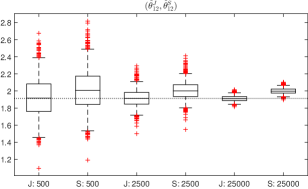
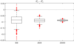
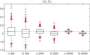
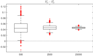
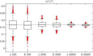
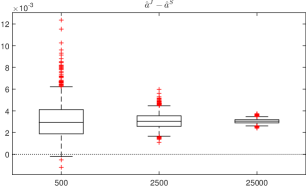
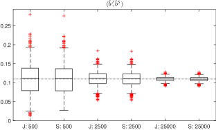
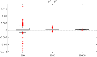
Figure 5: Box plots of joint (J) and sequential (S) ML estimates and their difference for sample sizes $N=500,2500,25000$, if the data is generated from $C_{1:3}$ in Example A.2 and the pair-copula families of the SVC are given by the corresponding PVC. The dotted line indicates the pseudo-true parameter and zero, respectively. The end of the whiskers is 0.953 times the inter-quartile range, corresponding to approximately 95% coverage if the data is generated by a normal distribution.

Note that $g$ is a sigmoid function, with $(g(0),g(1))=(-0.2,\sqrt{7}/5)$, so that Spearman’s rho of the conditional copula $C^{{\text{Sar}}}\!(g(u_{2}))$ varies in the interval $(g(0),g(1))=(-0.2,\sqrt{7}/5)$ because $\rho_{C^{\text{Sar}}}=\alpha$. Figure 5 shows that the difference between step-by-step and joint ML estimates for the two parameters of the first copula in the first tree is already (individually) significant at the 5% level if the sample size is 500 observations. Thus, the difference between step-by-step and joint ML estimates can be relevant for moderate sample sizes if the variation in the conditional copula is strong enough. Once again, the difference between step-by-step and joint ML estimates is less pronounced for the parameters of $C^{\text{\tiny SVC}}_{13;2}$ but it also becomes highly significant with sufficient sample size.

References

- Nelsen [2006] R. B. Nelsen, An introduction to copulas, Springer series in statistics, Springer, New York, 2006.
- Joe [1997] H. Joe, Multivariate models and dependence concepts, Chapman & Hall, London, 1997.
- McNeil et al. [2005] A. J. McNeil, R. Frey, P. Embrechts, Quantitative risk management, Princeton series in finance, Princeton Univ. Press, Princeton NJ, 2005.
- Joe [1996] H. Joe, Families of m-Variate Distributions with Given Margins and m(m-1)/2 Bivariate Dependence Parameters, Lecture Notes-Monograph Series 28 (1996) 120–141.
- Aas et al. [2009] K. Aas, C. Czado, A. Frigessi, H. Bakken, Pair-Copula Constructions of Multiple Dependence, Insurance: Mathematics and Economics 44 (2009) 182–198.
- Dißmann et al. [2013] J. Dißmann, E. C. Brechmann, C. Czado, D. Kurowicka, Selecting and estimating regular vine copulae and application to financial returns, Computational Statistics & Data Analysis 59 (2013) 52–69.
- Grothe and Nicklas [2013] O. Grothe, S. Nicklas, Vine constructions of Lévy copulas, Journal of Multivariate Analysis 119 (2013) 1–15.
- Joe et al. [2010] H. Joe, H. Li, A. K. Nikoloulopoulos, Tail dependence functions and vine copulas, Journal of Multivariate Analysis 101 (2010) 252–270.
- Kauermann and Schellhase [2013] G. Kauermann, C. Schellhase, Flexible pair-copula estimation in D-vines using bivariate penalized splines, Statistics and Computing (2013) 1–20.
- Nikoloulopoulos et al. [2012] A. K. Nikoloulopoulos, H. Joe, H. Li, Vine copulas with asymmetric tail dependence and applications to financial return data, Computational Statistics & Data Analysis 56 (2012) 3659–3673.
- Aas and Berg [2009] K. Aas, D. Berg, Models for construction of multivariate dependence – a comparison study, The European Journal of Finance 15 (2009) 639–659.
- Fischer et al. [2009] M. Fischer, C. Köck, S. Schlüter, F. Weigert, An empirical analysis of multivariate copula models, Quantitative Finance 9 (2009) 839–854.
- Hobæk Haff et al. [2010] I. Hobæk Haff, K. Aas, A. Frigessi, On the simplified pair-copula construction – Simply useful or too simplistic?, Journal of Multivariate Analysis 101 (2010) 1296–1310.
- Stöber et al. [2013] J. Stöber, H. Joe, C. Czado, Simplified pair copula constructions—Limitations and extensions, Journal of Multivariate Analysis 119 (2013) 101–118.
- Bergsma [2004] W. Bergsma, Testing conditional independence for continuous random variables, 2004. URL: http://eprints.pascal-network.org/archive/00000824/.
- Gijbels et al. [2015a] I. Gijbels, M. Omelka, N. Veraverbeke, Estimation of a Copula when a Covariate Affects only Marginal Distributions, Scandinavian Journal of Statistics 42 (2015a) 1109–1126.
- Gijbels et al. [2015b] I. Gijbels, M. Omelka, N. Veraverbeke, Partial and average copulas and association measures, Electronic Journal of Statistics 9 (2015b) 2420–2474.
- Spanhel and Kurz [2016] F. Spanhel, M. S. Kurz, The partial copula: Properties and associated dependence measures, Statistics & Probability Letters 119 (2016) 76 – 83.
- Portier and Segers [2015] F. Portier, J. Segers, On the weak convergence of the empirical conditional copula under a simplifying assumption, ArXiv e-prints (2015). arXiv:1511.06544.
- Nagler and Czado [2016] T. Nagler, C. Czado, Evading the curse of dimensionality in nonparametric density estimation with simplified vine copulas, Journal of Multivariate Analysis 151 (2016) 69 -- 89.
- Kurz and Spanhel [2017] M. S. Kurz, F. Spanhel, Testing the simplifying assumption in high-dimensional vine copulas, ArXiv e-prints (2017). arXiv:1706.02338.
- Bedford and Cooke [2002] T. Bedford, R. M. Cooke, Vines: A New Graphical Model for Dependent Random Variables, The Annals of Statistics 30 (2002) 1031--1068.
- Kurowicka and Joe [2011] D. Kurowicka, H. Joe (Eds.), Dependence modeling, World Scientific, Singapore, 2011.
- Kurowicka and Cooke [2006] D. Kurowicka, R. Cooke, Uncertainty analysis with high dimensional dependence modelling, Wiley, Chichester, 2006.
- Hobæk Haff [2013] I. Hobæk Haff, Parameter estimation for pair-copula constructions, Bernoulli 19 (2013) 462--491.
- Patton [2006] A. J. Patton, Modelling Asymmetric Exchange Rate Dependence, International Economic Review 47 (2006) 527--556.
- Acar et al. [2012] E. F. Acar, C. Genest, J. Nešlehová, Beyond simplified pair-copula constructions, Journal of Multivariate Analysis 110 (2012) 74--90.
- Krupskii and Joe [2013] P. Krupskii, H. Joe, Factor copula models for multivariate data, Journal of Multivariate Analysis 120 (2013) 85--101.
- Hobæk Haff [2012] I. Hobæk Haff, Comparison of estimators for pair-copula constructions, Journal of Multivariate Analysis 110 (2012) 91--105.
- Fermanian and Wegkamp [2012] J.-D. Fermanian, M. H. Wegkamp, Time-dependent copulas, Journal of Multivariate Analysis 110 (2012) 19--29.
- Schepsmeier et al. [2016] U. Schepsmeier, J. Stoeber, E. C. Brechmann, B. Graeler, T. Nagler, T. Erhardt, VineCopula: Statistical Inference of Vine Copulas, 2016. URL: https://CRAN.R-project.org/package=VineCopula, r package version 2.0.5.
- Hobæk Haff and Segers [2015] I. Hobæk Haff, J. Segers, Nonparametric estimation of pair-copula constructions with the empirical pair-copula, Computational Statistics & Data Analysis 84 (2015) 1--13.
- Kauermann et al. [2013] G. Kauermann, C. Schellhase, D. Ruppert, Flexible Copula Density Estimation with Penalized Hierarchical B-splines, Scandinavian Journal of Statistics 40 (2013) 685--705.
- White [1982] H. White, Maximum Likelihood Estimation of Misspecified Models, Econometrica 50 (1982) 1--25.
- Spanhel and Kurz [2016] F. Spanhel, M. S. Kurz, Estimating parametric simplified vine copulas, Working paper (2016).
- Mesfioui and Quessy [2008] M. Mesfioui, J.-F. Quessy, Dependence structure of conditional Archimedean copulas, Journal of Multivariate Analysis 99 (2008) 372--385.
- Remillard [2013] B. Remillard, Statistical methods for financial engineering, CRC Press, Boca Raton, Fl., 2013.