Modelling the chemistry of star forming filaments – I. H₂ and CO chemistry

Abstract

We present simulations of star forming filaments incorporating on of the largest chemical network used to date on-the-fly in a 3D-MHD simulation. The network contains 37 chemical species and about 300 selected reaction rates. For this we use the newly developed package KROME (Grassi et al., 2014). We combine the KROME package with an algorithm which allows us to calculate the column density and attenuation of the interstellar radiation field necessary to properly model heating and ionisation rates. Our results demonstrate the feasibility of using such a complex chemical network in 3D-MHD simulations on modern supercomputers. We perform simulations with different strengths of the interstellar radiation field and the cosmic ray ionisation rate. We find that towards the centre of the filaments there is gradual conversion of hydrogen from H to H₂ as well as of C⁺ over C to CO. Moreover, we find a decrease of the dust temperature towards the centre of the filaments in agreement with recent HERSCHEL observations.

1 Introduction

Modelling the chemical evolution of the gas during the process of star formation on various scales is a numerically and theoretically challenging task. On the one hand, it requires to solve a large set of reaction equations with sufficient accuracy, which is computationally extremely demanding. On the other hand in depth knowledge about the necessary reactions and their corresponding rates is required, which involves laboratory work and quantum mechanical calculations.

Nonetheless, the chemical state of the gas and the associated cooling and heating processes are required to properly model the thermodynamical evolution of the gas and to make accurate predictions via synthetic observations. In particular in the latter case it is common to use fixed conversion factors to e.g. obtain the number density of a particular molecular species from the gas density which, however, is a severe oversimplification and might not be accurate enough.

Several authors have incorporated reduced chemical networks in their 3D, magneto-hydrodynamical (MHD) simulations (e.g. Clark et al., 2013; Smith et al., 2014; Walch et al., 2015; Hocuk et al., 2016). The newly designed chemistry package KROME (Grassi et al., 2014) is a versatile package which allows the user to incorporate chemistry in MHD simulations in a very efficient manner and simultaneously guarantees the freedom to choose any desired network as well as its associated cooling and heating processes. It is therefore a good choice to model the complex chemical evolution of star forming regions.

Recently, the importance of filamentary structures in star forming clouds has been re-emphasized (e.g. André et al., 2010). These filaments result from the interaction of gravity and turbulence and harbour pre- and protostellar cores (for recent numerical works see e.g. Gómez & Vázquez-Semadeni, 2014; Smith et al., 2014; Kirk et al., 2015). Recent observations of molecular line and dust emission provide a wealth of information about the properties of these filaments, like e.g. the thermodynamical state, the typical extension, and fragmentation of the filaments. Numerical simulations, however, often lack the detailed description of the chemical state and can thus be compared only indirectly to the observations. This and the fact that filaments appear to be ubiquitous in the star formation process make them an optimal target to test the feasibility of using a detailed chemical network in fully self-consistent 3D-MHD simulations.

The outline of the paper is as follows: In Section 2 we briefly discuss the initial conditions, in Section 3 we describe the employed chemical network and heating and cooling processes. In Section 4 we describe the time evolution of a fiducial run and study the impact of the radiation field on the chemical and thermal evolution of the filaments. In Section 5 we compare with observations and give details about the computational cost before we summarize our results.

2 Initial conditions and FLASH solver

The simulations presented here use the same initial conditions and numerical methods – except the chemistry and cooling/heating processes – as those presented in Seifried & Walch (2015). Here we briefly summarize the main points. The simulations are performed with the astrophysical code FLASH 4.2.2 (Dubey et al., 2008). We solve the equations of ideal MHD using a maximum resolution of 40.3 AU. The Poisson equation for gravity is solved using a multipole method based on a Barnes-Hut tree (Wünsch et al., 2015, in prep.).

The simulated filaments have an initial width of about 0.1 pc following a Plummer-like density profile along the radial direction. The filaments have a length of 1.6 pc and a mass per unit length of 75 M_☉/pc. This corresponds to about three times the critical mass per unit length (Ostriker, 1964) of

$$(M/L)_{\mathrm{crit}}=\frac{2c_{\mathrm{s}}^{2}}{G}\,,$$ (1)

which is why the filaments are unstable against collapse along the radial direction and subject to subsequent fragmentation. The initial central density of the filaments is $3\times 10^{-19}$ g cm^-3.

Recent observations have shown that filaments have magnetic fields which can be directed either along or perpendicular to the filament (e.g. Sugitani et al., 2011; Li et al., 2013; Palmeirim et al., 2013), which is why we test both magnetic field orientations. We take the initial magnetic field strength in the centre of the filament to be 40 $\mu$G, in agreement with recent observations (e.g. Sugitani et al., 2011). The field is uniform in strength for the perpendicular case and declines outwards in the parallel case proportional to $\rho^{0.5}$. In addition, we superimpose a transonic turbulent velocity field (for more details see Seifried & Walch, 2015).

The strength of the interstellar radiation field (ISRF) and the cosmic ray ionisation rate (CRIR) influence the reaction rates as well as the heating of dust, which is taken into account by the chemistry package (see Online Material). Since, however, the strength of the ISRF and the CRIR can vary locally in our Galaxy, we perform simulations with different values. In our fiducial run we apply a CRIR of $1.3\times 10^{-17}$ s^-1 (e.g. Vastel et al., 2006) and an ISRF corresponding to 1.7 times the Habing flux (G₀ = 1.7, Draine, 1978). Since for the CRIR also significantly higher values are found (e.g. Caselli et al., 1998; Ceccarelli et al., 2011), we perform a second pair (perpendicular and parallel magnetic fields) of simulations with a CRIR of $1\times 10^{-16}$ s^-1 and G₀ = 1.7. In the third set of simulations we additionally increase the ISRF by a factor of 5, i.e. G₀ = 8.5. Hence, in total we have a set of six simulations with different (initial) conditions.

3 The chemical network

In order to model the chemical evolution of the gas, we use the KROME package (Grassi et al., 2014), which in principle allows to model any desired chemical network. The network used contains 37 species and 287 reactions including different forms of hydrogen and carbon bearing species like H⁺, H, H₂, C⁺, C, and CO but also more complex species like e.g. HCO⁺, H₂O, or the cosmic ray tracer H${}_{3}^{+}$. In particular, the network allows for a very detailed description of the formation of CO and H₂ (also including the formation of H₂ on dust). We assume that all elements heavier than He are depleted with respect to their cosmic abundances using values given by Flower et al. (2005) typical for dense molecular gas. Initially all elements are in their atomic form. More details about the used species, reactions, and initial abundances are provided in the Online Material. In addition, we benchmark our implementation (network and radiative transfer) against the KOSMA-$\tau$ PDR code for two tests presented in Röllig et al. (2007) and find very good agreement.

The strength of the ISRF and the CRIR are needed to model the chemical evolution as well as the heating and cooling processes properly. In particular, the ISRF experiences an attenuation when travelling through the gas. We calculate the attenuation in the FLASH code with the TreeCol algorithm (Clark et al., 2012; Wünsch et al., 2015, in prep.). For each cell in the computational domain we compute the total (H + H₂), H₂, and the CO column densities in 48 directions. We take the geometrical average and obtain the mean column densities, N_H,tot, N${}_{\mathrm{H_{2}}}$, and N_CO, as well as the visual extinction, $A_{V}$, and the self-shielding factors for H₂ and CO photodissociation (Glover et al., 2010, see also section 2.2.1 and 2.2.2 in Walch et al. (2015) for a more detailed technical description). The attenuation of the ISRF also affects the photoelectric (PE) heating due to dust particles, which is taken into account by scaling the strength of the ISRF with G₀ $\times$ exp(-2.5 $A_{V}$).

The cooling rate due to line emission of CO is provided by K. Omukai in tabulated form based on the results of Neufeld & Kaufman (1993) and Omukai et al. (2010). The actual rate in each cell depends on N_CO and the local gas density and gas temperature, $T_{\mathrm{gas}}$ . We also use these tabulated rates to calculate the cooling due to ¹³CO and C¹⁸O by downscaling N_CO and the according cooling rates by 69 and 557, respectively (Wilson, 1999).

Finally, for calculating the dust temperature, $T_{\mathrm{dust}}$, we take into account the transfer of energy from gas to grains via collisions, which also affects $T_{\mathrm{gas}}$ itself, heating of the grains due to the ISRF, and cooling of dust grains via black-body radiation. In each timestep, we calculate the equilibrium dust temperature for all three processes after the chemistry update is done. We emphasize that a more detailed description of all cooling and heating processes used and their coupling to the ISRF and the CRIR is provided in the Online Material.

4 Results

4.1 Time evolution of a fiducial run

Before we start the different simulations, we evolve the chemistry in each cell for 500 kyr, during which the hydrodynamical evolution is turned off, i.e. only $T_{\mathrm{gas}}$, $T_{\mathrm{dust}}$, and the chemical composition are updated. Since at densities of about 10⁵ cm^-3 the typical timescale for H₂ formation on dust grains is of the order of 100 kyr, 500 kyr are sufficient to reach a rough chemical equilibrium. After this initial relaxation phase, each simulation is followed for 300 kyr.

In the following, we present the time evolution of the run with a parallel magnetic field, G₀ = 1.7, and a CRIR of 1.3 $\times$ 10^-17 s^-1. In Fig. 1 we plot the spatial distribution of H, H₂, C, and CO at the end of the simulation, which reveals some differences in the radial distribution. Whereas H₂ and CO are concentrated towards the centre of the filament, H and C are more extended. Moreover, there is a clear impact of the initial turbulence field on the distribution of the chemical species, causing strong local variations.

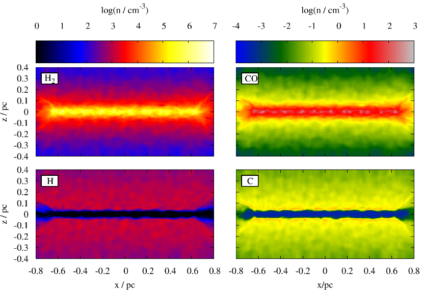
Figure 1: Spatial distribution of H, H₂, C, and CO at the end of the simulation with a parallel magnetic field, G₀ = 1.7, and a CRIR of 1.3 $\times$ 10^-17 s^-1 along a slice through the centre of the filament.

The radial density profiles of H₂, H, H⁺, CO, C, and C⁺ at 4 different times are shown in Fig. 2. In order to smooth out local fluctuations, we have averaged the densities along the major axis of the filament.

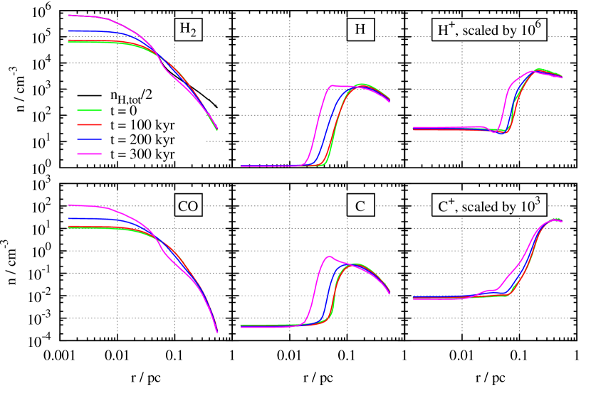
Figure 2: From left to right: Radial dependence of the density of H₂, H, H⁺ (top row), and CO, C, and C⁺ (bottom row) at t = 0, 100, 200, and 300 kyr after the start of the same simulation as in Fig. 1. Note that at t = 0, the chemical distribution corresponds to that after an initial relaxation phase of 500 kyr. In order to use the same $y$-axis, $n_{\mathrm{H^{+}}}$ and $n_{\mathrm{C^{+}}}$ are scaled up by a factor of 10⁶ and 10³, respectively. The black line in the upper left panel shows the total hydrogen density divided by two.

The constant increase of the central number densities of H₂ and CO over time is caused by the contraction of the filament along the radial direction. On the other hand, the abundance of H, H⁺, C, and C⁺ remain almost constant over time as they recombine when the filament becomes denser. In the upper left panel we also show the number density of all H atoms (divided by two in order to be comparable to $n_{\mathrm{H_{2}}}$), which represents the shape of the mass density profile. In the centre of the filament most of the hydrogen is bound in H₂, only outside $\sim$ 0.1 pc, where the black and purple line start to differ, hydrogen mainly occurs in atomic form. Hence, there is a gradual conversion of H to H₂ towards the centre of the filament as well as of C⁺ over C to CO, with $n_{\mathrm{C}}$ exceeding $n_{\mathrm{CO}}$ at $\sim$ 0.1 pc as well. This agrees with the picture obtained from Fig. 1 that H and C envelop H₂ and CO and is in good agreement with theoretical predictions of PDRs (e.g. van Dishoeck & Black, 1988). We note that a similar result was also found by Clark et al. (2013).

4.2 Impact of the ISRF and the CRIR

Next, we study the influence of the ISRF and CRIR on the properties of the filaments. In Fig. 3 we plot the radial dependence of H₂, H, and H⁺ (top row), as well as of CO, C, and C⁺ (middle row) and of $T_{\mathrm{gas}}$ and $T_{\mathrm{dust}}$, (bottom row) at the end of each of the six simulations. On the left we show the runs with a perpendicular magnetic field, on the right runs with a parallel magnetic field. As already seen in Fig. 2, we find a gradual conversion of H to H₂, and C⁺ over C to CO towards centre of the filaments for all runs.

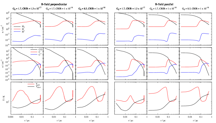
Figure 3: Radial dependence of H₂, H, H⁺ (top row), CO, C, C⁺ (middle row) as well as the gas and dust temperature (bottom row) at the end of each simulation. Left panel: runs with a perpendicular magnetic field. Right panel: runs with a parallel magnetic field.

Increasing the CRIR results in a somewhat higher ionisation reflected by the abundances of H⁺ and C⁺. Moreover, at high densities $n_{H}$ is around a few times 1 cm^-3 with somewhat higher values for higher CRIR and thus in good agreement with theoretical predictions (e.g. Tielens, 2005). Also $T_{\mathrm{gas}}$ shows a slight increase with increasing CRIR, which is due to the larger amount of energy released by various dissociation reactions caused by cosmic rays.

Increasing the strength of the ISRF only marginally affects the chemical composition of the gas. However, $T_{\mathrm{gas}}$ and $T_{\mathrm{dust}}$ are increased by a few Kelvin, which is most likely due to the increased PE heating. Interestingly, we find that for all runs $T_{\mathrm{dust}}$ decreases towards the centre of the filaments. We attribute this to the progressive attenuation of the ISRF – mainly responsible for dust heating – towards the centre of the filament (see also Clark et al., 2013). The gas temperature, however, shows a significant increase between 0.01 pc and 0.1 pc. Investigating the dynamics of the filaments, we find that this corresponds to an accretion shock where the infalling gas is decelerated.

As shown in Seifried & Walch (2015) the magnetic field has a strong impact on the dynamical evolution of the filament, which is partly also reflected in the chemical composition. In particular the two runs with G₀ = 1.7 and a CRIR of 1.3 $\times$ 10^-17 s^-1 show a somewhat different chemical composition with respect to atomic hydrogen and carbon. A more significant difference can be seen in the gas temperature, which as mentioned before, is tightly linked to the infall velocities, which in turn depends on the configuration of the magnetic field (Seifried & Walch, 2015).

5 Discussion and conclusions

5.1 Physical interpretation

As shown in Fig. 3, $T_{\mathrm{dust}}$ decreases towards the centre of the filament in all runs, which was recently also found in observations (Arzoumanian et al., 2011; Palmeirim et al., 2013; Li et al., 2014). From the averaged quantities (Figs. 2 and 3) we can now obtain the polytropic index $\gamma$ of the dust by assuming a polytropic relation $T_{\mathrm{dust}}\propto\rho^{\gamma-1}$. We note that we rather use a relation between the $T_{\mathrm{dust}}$ (instead of $T_{\mathrm{gas}}$) and $\rho$ in order to be able to directly compare our results to HERSCHEL observations: by visual inspection of the $T_{\mathrm{dust}}$ vs. $\rho$ plots (see Online Material), we find $\gamma$ to be in a range from 0.9 to 0.95, which is in good agreement with Palmeirim et al. (2013). We again emphasize that $T_{\mathrm{gas}}$ and $T_{\mathrm{dust}}$ are markedly different, which requires independent measurements for both quantities in observations. We attribute this to the fact that the collisional coupling between gas and dust at $n\sim 10^{5}-10^{6}$ cm^-3 is not yet strong enough to assure similar temperatures, although our results suggest that $T_{\mathrm{dust}}$ and $T_{\mathrm{gas}}$ approach each other towards the center of the filaments.

By inspecting Fig. 3 it can also be seen that the ratio $R=\frac{n_{\mathrm{CO}}}{n_{\mathrm{H_{2}}}}$ is not constant along the radial direction. There is a strong decline of $R$ with increasing radius of about 2 orders of magnitude, which is due to the fact that the formation of CO happens at somewhat smaller radii (i.e. higher gas column densities) than that of H₂. This variation in $R$ most likely also affects the value of the X-factor, which is used to convert CO luminosities into H₂ column densities. Our work therefore suggests that caution is recommended when using CO line intensities to obtain total gas masses. Furthermore, varying CRIR and ISRF mainly affects $R$ at radii larger than 0.05 pc. In the centre of the filament, however, $R$ is comparable for all our runs with a value around $1.5\times 10^{-4}$, and thus in good agreement with observations (see Tielens, 2013, for a recent review) despite our simplified depletion description. We note that the variation of $R$ over time is rather small, independent of the considered run.

Finally, we emphasise that also abundances of other species like H${}_{3}^{+}$, H₂O, OH, or CH included in the network seem to be in reasonable agreement with observations (e.g. Tielens, 2013). This is a significant step forward compared to smaller chemical networks used in previous works (e.g. Clark et al., 2013; Smith et al., 2014; Walch et al., 2015). We postpone a more in-depth discussion of these species to a subsequent paper.

5.2 Numerical cost/Performance

The simulations were carried out on computing nodes with 2 - 5 GB memory per CPU, which corresponds to state-of-the-art computing nodes at modern supercomputing facilities (see Acknowledgements for which facilities were used). In order to estimate the increase of computational power required, we compare our runs with an isothermal ($T$ = 15 K) simulation without a chemical network, which is also evolved for 300 kyr. The slightly different thermodynamical evolution of the filaments in runs with and without the network results in slightly different timesteps as well as different numbers of cells in the simulation domain, which cannot be avoided. However, these differences affect the cost estimates only marginally. Overall, we find that the inclusion of the network (including heating and cooling processes) increases the computation costs per timestep by roughly a factor of 7. However, tabulating the reaction rate coefficients, which avoids the repeated evaluation of the exponential function, reduces the cost increase to about a factor of 5.

Altogether we argue that – considering the ever increasing computing power, the higher accuracy as well as the significant gain of additional physical and chemical information – it seems feasible and necessary for the future to perform simulations with large chemical networks.

5.3 Conclusions and outlook

We present first results of simulations of star forming filaments using one of the largest chemical network ever applied in 3D-MHD simulations. For this we combine the versatile chemistry package KROME (Grassi et al., 2014) with the TreeCol algorithm (Clark et al., 2012; Wünsch et al., 2015, in prep.), which allows us to self-consistently calculate the optical depth and shielding parameters in the simulation domain, which in turn is required to properly determine dissociation and photoionization reactions. The network contains 37 species and 28.pdf7 thoroughly selected reactions. We show that in terms of memory consumption such simulations are feasible on modern supercomputers. Despite an increase of computation costs by a factor of $\sim$ 5 – 7, we argue that the significant gain of physical and chemical information justifies the usage of large chemical networks in future simulations.

Concerning the chemical composition as well as the thermodynamical behaviour of the simulated filaments, the results appear to be promising and in good agreement with observational results. In particular, we show that there is a gradual conversion of H to H₂ as well as of C⁺ over C to CO towards the centre of the filaments. Moreover, we find that the dust temperature $T_{\mathrm{dust}}$ decreases towards the centre of the filament following a polytropic relation $T_{\mathrm{dust}}\propto\rho^{\gamma-1}$ with $\gamma\simeq 0.9-0.95$ in agreement with recent observations (Arzoumanian et al., 2011; Palmeirim et al., 2013; Li et al., 2014). Furthermore, we show that the dust and gas temperature can be markedly different even at densities of $n\sim 10^{5}-10^{6}$ cm^-3.

This work paves the way for many future applications: The detailed chemical modelling will allow us to produce synthetic observations of several molecular lines as well as of continuum emission. Filament widths obtained from these synthetic observations allow us to study how well a projected (2D–) width matches the actual (3D–) width of the filament obtained directly from the simulation data. Furthermore, the simulations can improve our understanding of the X-factor required for the mass determination of gaseous objects. Moreover, the network will allow us to study in detail the evolution of other molecules like H₂O or the cosmic ray tracer H${}_{3}^{+}$, which, due to space limitations, we could not discuss here. We also note that we plan to include even more complex chemical networks. In particular, the inclusion of nitrogen, a constituent of a number of important observational tracers, is of large interest. Finally, we plan to improve our treatment of CO freeze-out in order to get a better handle on the X-factor.

See pages 1-6 of DSeifried_online_material.pdf

References

- André et al. (2010) André, P., Men’shchikov, A., Bontemps, S., et al. 2010, A&A, 518, L102
- Arzoumanian et al. (2011) Arzoumanian, D., André, P., Didelon, P., et al. 2011, A&A, 529, L6
- Caselli et al. (1998) Caselli, P., Walmsley, C. M., Terzieva, R., & Herbst, E. 1998, ApJ, 499, 234
- Ceccarelli et al. (2011) Ceccarelli, C., Hily-Blant, P., Montmerle, T., et al. 2011, ApJ, 740, L4
- Clark et al. (2012) Clark, P. C., Glover, S. C. O., & Klessen, R. S. 2012, MNRAS, 420, 745
- Clark et al. (2013) Clark, P. C., Glover, S. C. O., Ragan, S. E., Shetty, R., & Klessen, R. S. 2013, ApJ, 768, L34
- Draine (1978) Draine, B. T. 1978, ApJS, 36, 595
- Dubey et al. (2008) Dubey, A., Fisher, R., Graziani, C., et al. 2008, in Astronomical Society of the Pacific Conference Series, Vol. 385, Numerical Modeling of Space Plasma Flows, ed. N. V. Pogorelov, E. Audit, & G. P. Zank, 145
- Flower et al. (2005) Flower, D. R., Pineau Des Forêts, G., & Walmsley, C. M. 2005, A&A, 436, 933
- Glover et al. (2010) Glover, S. C. O., Federrath, C., Mac Low, M.-M., & Klessen, R. S. 2010, MNRAS, 404, 2
- Gómez & Vázquez-Semadeni (2014) Gómez, G. C. & Vázquez-Semadeni, E. 2014, ApJ, 791, 124
- Grassi et al. (2014) Grassi, T., Bovino, S., Schleicher, D. R. G., et al. 2014, MNRAS, 439, 2386
- Hocuk et al. (2016) Hocuk, S., Cazaux, S., Spaans, M., & Caselli, P. 2016, MNRAS, 456, 2586
- Kirk et al. (2015) Kirk, H., Klassen, M., Pudritz, R., & Pillsworth, S. 2015, ApJ, 802, 75
- Li et al. (2014) Li, D. L., Esimbek, J., Zhou, J. J., et al. 2014, A&A, 567, A10
- Li et al. (2013) Li, H.-b., Fang, M., Henning, T., & Kainulainen, J. 2013, MNRAS, 436, 3707
- Neufeld & Kaufman (1993) Neufeld, D. A. & Kaufman, M. J. 1993, ApJ, 418, 263
- Omukai et al. (2010) Omukai, K., Hosokawa, T., & Yoshida, N. 2010, ApJ, 722, 1793
- Ostriker (1964) Ostriker, J. 1964, ApJ, 140, 1056
- Palmeirim et al. (2013) Palmeirim, P., André, P., Kirk, J., et al. 2013, A&A, 550, A38
- Röllig et al. (2007) Röllig, M., Abel, N. P., Bell, T., et al. 2007, A&A, 467, 187
- Seifried & Walch (2015) Seifried, D. & Walch, S. 2015, MNRAS, 452, 2410
- Smith et al. (2014) Smith, R. J., Glover, S. C. O., & Klessen, R. S. 2014, MNRAS, 445, 2900
- Sugitani et al. (2011) Sugitani, K., Nakamura, F., Watanabe, M., et al. 2011, ApJ, 734, 63
- Tielens (2005) Tielens, A. G. G. M. 2005, The Physics and Chemistry of the Interstellar Medium
- Tielens (2013) Tielens, A. G. G. M. 2013, Reviews of Modern Physics, 85, 1021
- van Dishoeck & Black (1988) van Dishoeck, E. F. & Black, J. H. 1988, ApJ, 334, 771
- Vastel et al. (2006) Vastel, C., Caselli, P., Ceccarelli, C., et al. 2006, ApJ, 645, 1198
- Walch et al. (2015) Walch, S., Girichidis, P., Naab, T., et al. 2015, MNRAS, 454, 238
- Wilson (1999) Wilson, T. L. 1999, Reports on Progress in Physics, 62, 143
- Wünsch et al. (2015, in prep.) Wünsch, R., Walch, S., Whitworth, A., & Dinnbier, F. 2015, in prep.