Effective resonant stability of Mercury

Abstract

Mercury is the unique known planet that is situated in a 3:2 spin-orbit resonance nowadays. Observations and models converge to the same conclusion: the planet is presently deeply trapped in the resonance and situated at the Cassini state $1$, or very close to it. We investigate the complete non-linear stability of this equilibrium, with respect to several physical parameters, in the framework of Birkhoff normal form and Nekhoroshev stability theory. We use the same approach adopted for the 1:1 spin-orbit case, published in Sansottera et al. (2014), with a peculiar attention to the role of Mercury’s non negligible eccentricity. The selected parameters are the polar moment of inertia, the Mercury’s inclination and eccentricity and the precession rates of the perihelion and node. Our study produces a bound to both the latitudinal and longitudinal librations (of 0.1 radians) for a long but finite time (greatly exceeding the age of the solar system). This is the so-called effective stability time. Our conclusion is that Mercury, placed inside the 3:2 spin-orbit resonance, occupies a very stable position in the space of these physical parameters, but not the most stable possible one.

1 Introduction

Mercury is the target of the BepiColombo mission, one of ESA’s cornerstone space missions, carried out in collaboration with the Japanese Aerospace Agency (JAXA). The spacecraft will be launched in 2017 and the orbit phase around Mercury is planned in 2024 (please refer to the BepiColombo webpage on the ESA website, http://sci.esa.in/bepicolombo, for updated information). Mercury has a peculiar feature: it is the only planet in the Solar System that is locked in a spin-orbit resonance, and the only object in the Solar System trapped in a 3:2 resonance. Indeed, the Moon and most of the regular satellites of the giant planets are found in 1:1 spin-orbit resonance.

The unique situation of Mercury can partly be explained by its large orbital eccentricity, see, e.g. Colombo & Shapiro (1966), Correia & Laskar (2004) and Celletti & Lhotka (2014). A more realistic tidal model has been used in Noyelles et al. (2014), where the authors demonstrate that capture in 3:2 resonance is possible on much shorter time-scales than previously thought.

These spin-orbit locked positions are usually named the (generalized) Cassini states ($1$ to $4$) and can be suitably described in terms of celestial dynamics, see, e.g. Colombo (1966), Peale (1969), Beletskii (1972) and Ward (1975). For an extension of the theory including the polar motion, see also Bouquillon et al. (2003).

The presence of a spin-orbit resonance allows to link the observational data of the orbital and rotational states with interior structure models, this is, for Mercury, the so-called Peale’s experiment, see Peale (1976).

The first observational confirmation of the Cassini State 1 for Mercury is due to Margot et al. (2007). Earth-based radar observations have confirmed its presence with high accuracy, see, e.g., Margot et al. (2012), where the authors demonstrate that the angle between the spin axis and the orbit normal, commonly referred to as obliquity, is consistent with the equilibrium hypothesis.

The same value of the obliquity was also determined by observational results from the NASA space mission MESSENGER that has also validated the 3:2 spin-orbit resonance to high accuracy, see Mazarico et al. (2014). The most recent value of the obliquity is $\varepsilon=2.06\pm 0.16$ arcmin, the orbital period is given by $T_{o}=87.969216879$ days $\pm 6$ seconds and the spin period is $T_{s}=58.64616\pm 0.000011$ days, that gives a ratio of about 3:2 to great accuracy.

It has been shown in Peale (2005) that small free oscillations around the exact equilibrium of the spin-orbit resonance are damped due to dissipative forces (mainly tidal effects and core-mantle friction) on a timescale of $10^{5}$ years. Any effect, that may bring Mercury away from exact spin-orbit resonance, like impacts, or any mechanism that may change Mercury’s internal mass and momenta distribution, will be counteracted on relatively short time scales. It is therefore reasonable to think that Mercury is currently situated at exact resonance or very close to it.

The question arises concerning the stability of the equilibrium itself in absence of dissipative forces to separate the influence of conservative non-linear effects from dissipative ones that act on shorter time-scales. The stability of the spin-orbit resonances has been numerically investigated in, e.g., Celletti & Chierchia (2000), Celletti & Voyatzis (2010) and Lhotka (2013) by means of stability maps. The non-linear stability of the Cassini states, in the 1:1 spin-orbit resonance, has been investigated in detail in Sansottera et al. (2014), by means of normal forms and Nekhoroshev type estimates. However, such an investigation of the non-linear stability, is still lacking for Mercury. We aim to carry out this study in the present paper. In particular, we are interested in the long-term non-linear stability: our goal is to produce a bound to both the latitudinal and longitudinal librations over long but finite times, namely an effective stability time.

Let us stress that in the present work we consider a realistic model in the mathematical sense. Indeed we are able to obtain significative analytic estimates on the stability time using the real physical parameters. However, in order to obtain a better physically realistic model, one should also take into account dissipative effects and planetary perturbations.

The long-term stability of perturbed proper rotations (rotations about a principal axis of inertia) in the sense of Nekhoroshev has been shown in Benettin et al. (2004). Furthermore, the authors suggest that their results may possibly be extended to the case of spin-orbit resonances. With our study we are able to demonstrate the long-term stability for motions that are trapped in a spin-orbit resonance and in particular the possible application of Nekhoroshev theory to Mercury.

We are able to give a definitive answer: the generalized Cassini state $1$, realized in terms of the 3:2 resonance, is practically stable on long time scales. However, we also demonstrate that the actual position of Mercury, in the parameter space, is placed in a very stable region, while not the most stable one. Indeed, altering some physical parameters, namely the polar moment of inertia factor, the inclination, the eccentricity and the precession rates of the perihelion and node, we found that the stability may change from a marginal amount to orders of magnitude, depending on the quantity of interest.

The present paper represents an extension of our previous work, developed for the 1:1 spin-orbit problems, see Sansottera et al. (2014), to the case of the 3:2 resonance and in particular to Mercury. The presence of a non negligible value for the eccentricity is a new aspect of the model to take into account. The mathematical basis of our work is represented by the Birkhoff normal form (1927) and the Nekhoroshev theory (1977; 1979).

Our approach is reminiscent of similar works on the same line, see, e.g., Giorgilli et al. (2009, 2010) and Sansottera et al. (2013), in which the authors gave an estimate of the long-time stability for the Sun-Jupiter-Saturn system and the planar Sun-Jupiter-Saturn-Uranus system, respectively.

This work is organized as follows: we introduce the spin-orbit model and its Hamiltonian formulation in Section 2. In Section 3 we describe an algorithm for the evaluation of the effective stability time via Birkhoff normal form. The application of our study to Mercury is presented in Section 4, while the physical interpretations and the possible extensions are reported in Section 5.

2 The model

We consider Mercury as a triaxial rigid body whose principal moments of inertia are $A$, $B$ and $C$, with $A\leq B<C$. We denote by $m$ and $R_{\rm e}$, the mass and equatorial radius of Mercury, respectively; and by $m_{0}$ the mass of the Sun.

We closely follow the notation adopted in Sansottera et al. (2014), that was also used in some previous studies on the same subject, see, e.g., Henrard & Schwanen (2004) for a general treatment of synchronous satellites, D’Hoedt & Lemaitre (2004) and Lemaitre et al. (2006) for Mercury, Noyelles et al. (2008) for the study of Titan, Lhotka (2013) for a symplectic mapping model and Noyelles & Lhotka (2013) for an investigation concerning the obliquity of Mercury during the BepiColombo space mission. Thus we refer to the quoted works for a detailed exposition and we just report here the key points so as to make the paper quite self-contained. First, we briefly recall how to express the Hamiltonian in the Andoyer-Delaunay set of coordinates, then we introduce the simplified spin-orbit model that represents the basis of our study.

2.1 Reference frames

The usual description of the spin-orbit motion requires four basic reference frames having their common origin in the center of mass of Mercury, see D’Hoedt & Lemaitre (2004). Namely, we need: (i) the inertial frame, $(X_{0},Y_{0},Z_{0})$, with $X_{0}$ and $Y_{0}$ lying in the ecliptic (or Laplace) plane; (ii) the orbital frame, $(X_{1},Y_{1},Z_{1})$, with $Z_{1}$ perpendicular to the orbit plane; (iii) the spin frame, $(X_{2},Y_{2},Z_{2})$, with $Z_{2}$ pointing to the spin axis direction and $X_{2}$ to the ascending node of the equatorial plane in the ecliptic plane; (iv) the body frame, (or figure frame), with $Z_{3}$ pointing into the direction of the axis of greatest inertia and $X_{3}$ of smallest inertia. In order to link the different frames we define $\nu_{01}$ as the direction along the ascending node of $(X_{0},Y_{0})$, in the plane $(X_{1},Y_{1})$, and $\nu_{23}$ as the direction of the ascending node between the planes $(X_{2},Y_{2})$ and $(X_{3},Y_{3})$.

We introduce two Euler angles: (i) the inertial obliquity, $K$, that is the angle between the axes $Z_{0}$ and $Z_{2}$; (ii) the wobble, $J$, between the axes $Z_{2}$ and $Z_{3}$. Moreover, we define the angles for the rotational motion: (i) the spin node, $h_{s}$, between $X_{0}$ and $X_{2}$, measured in the plane $(X_{0},Y_{0})$; (ii) the figure node, $g_{s}$, between $\nu_{23}$ and $X_{3}$, measured in the plane $(X_{2},Y_{2})$; (iii) the rotation angle, $l_{s}$, between $\nu_{23}$ and $X_{3}$, measured in the plane $(X_{3},Y_{3})$.

For the orbital dynamics, we introduce: (i) the longitude of the ascending node, $\Omega$, that gives the direction of $\nu_{01}$ measured in the plane $(X_{0},Y_{0})$; (ii) the inclination, $i$, being the angle between the axes $Z_{0}$ and $Z_{1}$; (iii) the perihelion argument, $\omega$, that defines the direction of the pericenter $X_{1}$ in the plane $(X_{1},Y_{1})$.

We report in Figure 1 the four reference frames and the angles defined above. On its basis we introduce the Andoyer-Delaunay canonical variables.

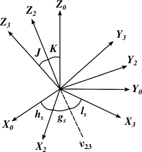
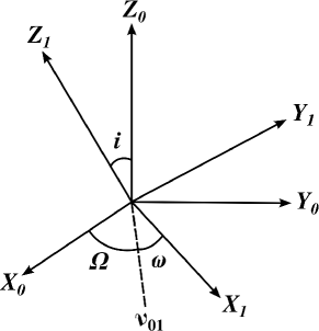
Figure 1: The four reference frames and the relevant angles related to the Andoyer (left) and Delaunay (right) canonical variables. See the text for more details.

2.2 Andoyer-Delaunay variables

We use the modified Andoyer variables in order to describe the rotational motion:

$$L_{1} =G_{s}\ , l_{1} =l_{s}+g_{s}+h_{s}\ ,$$ (1)

$$L_{2} =G_{s}-L_{s}\ , l_{2} =-l_{s}\ ,$$

$$L_{3} =G_{s}-H_{s}\ , l_{3} =-h_{s}\ ,$$

where $G_{s}$ denotes the norm of the spin angular momentum, $L_{s}=G_{s}\cos{J}$ and $H_{s}=G_{s}\cos{K}$.

For the orbital motion, we use the modified Delaunay variables, namely

$$L_{4} =L_{o}\ , l_{4} =M+\omega+\Omega\ ,$$ (2)

$$L_{5} =L_{o}-G_{o}\ , l_{5} =-\omega-\Omega\ ,$$

$$L_{6} =G_{o}-H_{o}\ , l_{6} =-\Omega\ ,$$

with $L_{o}=m\sqrt{\mu a}$, $G_{o}=L_{o}\sqrt{1-e^{2}}$, and $H_{o}=G_{o}\cos{i}$. As usual, $\mu=\mathcal{G}(m+m_{0})$ where $\mathcal{G}$ is the gravitational constant, $a$ is the semi-major axis, $e$ the eccentricity, $i$ the inclination and $M$ the mean anomaly. Let us remark that $L_{5}$ and $L_{6}$ are related to the eccentricity, $e$, and inclination, $i$, respectively. From now on, we assume that the spin-axis is aligned with the line of figure, i.e., $J=0$, and that we can neglect motion related to the conjugated variables $(L_{2},l_{2})$. Indeed, the polar motion of Mercury is assumed to be very small, see, e.g., Noyelles et al. (2010). Taking into account the 3:2 spin-orbit resonance, we introduce the resonant variables $\Sigma=(\Sigma_{1},\Sigma_{3})$, $\sigma=(\sigma_{1},\sigma_{3})$ by using the generating function

$$S_{3:2}=\Sigma_{1}\left(l_{1}-\frac{3}{2}\big{(}l_{4}+l_{5}\big{)}+l_{5}\right)+\Sigma_{3}\left(l_{3}-l_{6}\right)\ .$$

Thus we get

$$\Sigma_{1} =L_{1}\ , \sigma_{1} =l_{1}-\frac{3}{2}\big{(}l_{4}+l_{5}\big{)}+l_{5}\ ,$$

$$\Sigma_{3} =L_{3}\ , \sigma_{3} =l_{3}-l_{6}\ .$$ (3)

Here, $\sigma_{1}$ and $\sigma_{3}$ refer to the longitudinal and latitudinal librations, respectively, around the exact resonant state, placed at $\sigma_{1}=\sigma_{3}=0$.

In our model, the orbital ellipse of Mercury is assumed to be frozen but uniformly precessing due to the interactions with the other planets of the solar system. We keep fixed the semi-major axis, the eccentricity and the inclination: this corresponds to fixing the values of $L_{4}$, $L_{5}$ and $L_{6}$. Denoting by $n$ the mean motion, by $\dot{\omega}$ the mean precession rate of the argument of perihelion, by $\dot{\Omega}$ the mean regression rate of the ascending node and, without loss of generality, setting $t_{0}=0$ as the time of the perihelion passage of Mercury, we have the trivial equations of motion for the conjugated angles: $l_{4}=nt$, $l_{5}=\dot{\omega}t$ and $l_{6}=\dot{\Omega}t$. In this setting, the generating function $S_{3:2}$ is a function of time. Therefore, in order to express the Hamiltonian in the resonant variables, we have to add also the time derivative of the generating function, $\partial S_{3:2}/\partial t$.

2.3 Hamiltonian formulation

Let us denote by ${\mathcal{H}}_{s}$ and ${\mathcal{H}}_{o}$ the rotational and orbital kinetic energy, respectively, then the kinetic part reads

$$\begin{split}{\mathcal{T}}&=\mathcal{H}_{s}+\mathcal{H}_{o}+\frac{\partial S_{3:2}}{\partial t}\\ &=\frac{\Sigma_{1}^{2}}{2C}-\frac{3}{2}n\Sigma_{1}-\Sigma_{1}\dot{\omega}+\left(\Sigma_{3}-\Sigma_{1}\right)\dot{\Omega}\ ,\end{split}$$

where $C$ is the Mercury’s largest moment of inertia.

The dominant contribution of the gravitational potential is mainly due to two spherical harmonics: $C_{20}=\frac{A+B-2C}{2mR_{\rm e}^{2}}$ and $C_{22}=\frac{B-A}{4mR_{\rm e}^{2}}$. Thus we consider the potential energy

$${\mathcal{V}}=-\frac{\mathcal{G}mm_{0}R_{\rm e}^{2}}{r^{3}}\Bigl{(}C_{20}P_{20}(\sin\varphi)+C_{22}P_{22}(\sin\varphi)\cos 2\lambda\Bigr{)}\ ,$$ (4)

where $P_{20}$, $P_{22}$ are the Legendre polynomials and $\varphi$, $\lambda$ are the co-latitude and longitude of Mercury, respectively, with $\lambda$ measured east-wards from $X_{2}$ ($X_{3}$). The expression of the potential ${\mathcal{V}}$, defined in the figure frame, into the inertial frame is straightforward. Following the approach developed in Noyelles & Lhotka (2013), we write ${\mathcal{V}}$ in terms of the resonant variables and perform an average over the mean orbital longitude $l_{4}$. We denote by $\langle{\mathcal{V}}\rangle$ the averaged potential and we refer to the previous paper for all the details. We just stress that here, as an extension to Noyelles & Lhotka (2013), we consider an expansion in the eccentricity up to order 8, while we only keep the time-independent harmonics in the definition of ${\langle\mathcal{V}\rangle}$, namely the ${\langle\mathcal{V}_{20}\rangle}$ and ${\langle\mathcal{V}_{22}\rangle}$ terms, defined there.

Denoting by $\langle T\rangle$ the averaged kinetic energy and introducing the averaged Hamiltonian ${\langle\mathcal{H}\rangle=\langle T\rangle+\langle\mathcal{V}\rangle}$, the equations of motion read

$$\dot{\Sigma}=-\frac{\partial{\langle\mathcal{H}\rangle}}{\partial\sigma}\ ,\quad\dot{\sigma}=+\frac{\partial{\langle\mathcal{H}\rangle}}{\partial\Sigma}\ .$$ (5)

Setting $\sigma=0$ we look for the equilibrium $\Sigma^{*}=\left(\Sigma_{1}^{*},\Sigma_{3}^{*}\right)$ by solving the equations

$$f_{1}\left(\Sigma\right)\equiv\frac{\partial{\langle\mathcal{H}\rangle}}{\partial\Sigma_{1}}\bigg{|}_{\sigma=0}\hskip-5.0pt=0\ ,\quad f_{2}\left(\Sigma\right)\equiv\frac{\partial{\langle\mathcal{H}\rangle}}{\partial\Sigma_{2}}\bigg{|}_{\sigma=0}\hskip-5.0pt=0\ ,$$ (6)

namely the Cassini state 1.

Let us remark that, expressing $f_{1}\left(\Sigma\right)$ and $f_{2}\left(\Sigma\right)$ as functions of $(G_{s},K)$ one obtains an implicit formula for the obliquity $\varepsilon=i-K$ in terms of the system parameters, see Noyelles & Lhotka (2013). Precisely, setting $c=C/(mR_{\rm e}^{2})$, at the equilibrium, the following equation holds true

$$c=\frac{n\sin(\varepsilon)\left(C_{20}H_{20}\cos(\varepsilon)+C_{22}H_{22}(\cos(\varepsilon)+1)\right)}{\dot{\Omega}\sin(i-\varepsilon)\left(\frac{2\dot{\Omega}\cos(i-\varepsilon)}{3n}+\frac{2\dot{\omega}}{3n}+1\right)}\ ,$$ (7)

where $H_{20}$ and $H_{22}$, truncated at order 8, are given by

$$H_{20} =-1-\frac{3e^{2}}{2}-\frac{15e^{4}}{8}-\frac{35e^{6}}{16}-\frac{315e^{8}}{128}\ ,$$

$$H_{22} =\frac{7e}{2}-\frac{123e^{3}}{16}+\frac{489e^{5}}{128}-\frac{1763e^{7}}{2048}\ .$$ (8)

This relation will be useful for the physical interpretation of the results in terms of fixed $\varepsilon$. Let us remark that equation (7) represents a generalization of the one in Peale (1981).

3 Stability at the Cassini state

We now aim to study the stability properties of the Cassini state. To be more specific, our goal is to give an estimate of the effective stability time around the equilibrium point. Hereinafter we follow the exposition given in Sansottera et al. (2014) for the 1:1 spin-orbit problem.

We perform a translation in order to put the equilibrium at the origin and an expansion of the averaged Hamiltonian in power series of $(\Sigma,\sigma)$, namely

$$H(\Sigma,\sigma)=H_{0}(\Sigma,\sigma)+\sum_{j>0}H_{j}(\Sigma,\sigma)\ ,$$ (9)

where $H_{j}$ is an homogeneous polynomial of degree $j+2$ in $(\Sigma,\sigma)\,$. In the latter equation the quadratic term, $H_{0}$, has been put apart from the other terms of the Hamiltonian in view of its relevance in the perturbative scheme.

3.1 The untangling transformation

The quadratic part of the Hamiltonian reads

$$H_{0}(\Sigma,\sigma)= \mu_{{\scriptscriptstyle\Sigma_{1}\Sigma_{1}}}\Sigma_{1}^{2}+2\mu_{{\scriptscriptstyle\Sigma_{1}\Sigma_{3}}}\Sigma_{1}\Sigma_{3}+\mu_{{\scriptscriptstyle\Sigma_{3}\Sigma_{3}}}\Sigma_{3}^{2}$$

$$+\mu_{{\scriptscriptstyle\sigma_{1}\sigma_{1}}}\sigma_{1}^{2}+2\mu_{{\scriptscriptstyle\sigma_{1}\sigma_{3}}}\sigma_{1}\sigma_{3}+\mu_{{\scriptscriptstyle\sigma_{3}\sigma_{3}}}\sigma_{3}^{2}\ .$$

We perform the so-called untangling transformation, see Henrard & Lemaître (2005), that permits to get rid of the mixed terms. Thus, in the new coordinates, $H_{0}$ takes the form

$$H_{0}(\Sigma^{\prime},\sigma^{\prime})=\mu^{\prime}_{{\scriptscriptstyle\Sigma_{1}^{\prime}\Sigma_{1}^{\prime}}}\Sigma_{1}^{\prime 2}+\mu^{\prime}_{{\scriptscriptstyle\sigma_{1}^{\prime}\sigma_{1}^{\prime}}}\sigma_{1}^{\prime 2}+\mu^{\prime}_{{\scriptscriptstyle\Sigma_{3}^{\prime}\Sigma_{3}^{\prime}}}\Sigma_{3}^{\prime 2}+\mu^{\prime}_{{\scriptscriptstyle\sigma_{3}^{\prime}\sigma_{3}^{\prime}}}\sigma_{3}^{\prime 2}\ .$$

Let us remark that if both $\mu^{\prime}_{{\scriptscriptstyle\Sigma_{1}^{\prime}\Sigma_{1}^{\prime}}}\mu^{\prime}_{{\scriptscriptstyle\sigma_{1}^{\prime}\sigma_{1}^{\prime}}}$ and $\mu^{\prime}_{{\scriptscriptstyle\Sigma_{3}^{\prime}\Sigma_{3}^{\prime}}}\mu^{\prime}_{{\scriptscriptstyle\sigma_{3}^{\prime}\sigma_{3}^{\prime}}}$ are positive, as it happens in our case, the quadratic part of the Hamiltonian represents a couple of harmonic oscillators.

It is now useful to perform a rescaling and introduce the polar coordinates,

$$\Sigma_{1}^{\prime} =\sqrt{2U_{1}/U_{1}^{*}}\cos(u_{1})\ ,\qquad\sigma_{1}^{\prime}=\sqrt{2U_{1}U_{1}^{*}}\sin(u_{1})\ ,$$ (10)

$$\Sigma_{3}^{\prime} =\sqrt{2U_{3}/U_{3}^{*}}\cos(u_{3})\ ,\qquad\sigma_{3}^{\prime}=\sqrt{2U_{3}U_{3}^{*}}\sin(u_{3})\ ,$$

where

$$U_{1}^{*}=\sqrt{\mu^{\prime}_{{\scriptscriptstyle\Sigma_{1}^{\prime}\Sigma_{1}^{\prime}}}/\mu^{\prime}_{{\scriptscriptstyle\sigma_{1}^{\prime}\sigma_{1}^{\prime}}}}\ ,\qquad\hbox{and}\qquad U_{3}^{*}=\sqrt{\mu^{\prime}_{{\scriptscriptstyle\Sigma_{3}^{\prime}\Sigma_{3}^{\prime}}}/\mu^{\prime}_{{\scriptscriptstyle\sigma_{3}^{\prime}\sigma_{3}^{\prime}}}}\ .$$

Thus, the quadratic part of the Hamiltonian is expressed in action-angle variables as

$$H_{0}=\omega_{u_{1}}U_{1}+\omega_{u_{3}}U_{3}\ ,$$

where $\omega_{u_{1}}$ and $\omega_{u_{3}}$ are the frequencies of the angular variables $u_{1}$ and $u_{3}$, respectively. Again, we use the shorthand notations $U=(U_{1},U_{3})\,$, $u=(u_{1},u_{3})$ and $\omega_{u}=(\omega_{u_{1}},\omega_{u_{3}})\,$.

In these new coordinates, the transformed Hamiltonian can be expanded in Taylor-Fourier series and reads

$$H^{(0)}(U,u)=\omega_{u}\cdot U+\sum_{j>0}H^{(0)}_{j}(U,u)\ ,$$ (11)

where the terms $H_{j}$ are homogeneous polynomials of degree $j/2+1$ in $U$, whose coefficients are trigonometric polynomials in the angles $u\,$.

Mathematically speaking, the Hamiltonian (11) describes a perturbed system of harmonic oscillators, where the perturbation is proportional to the distance from the equilibrium. We now aim to investigate the stability around this equilibrium in the light of Nekhoroshev theory, introducing the so-called effective stability time.

3.2 Effective stability via Birkhoff normal form

Following a quite standard approach, we first construct the Birkhoff normal form for the Hamiltonian (11) and then give an estimate of the stability time.

The Hamiltonian is in normal form at order $r$ if

$$H^{(r)}(U,u)=Z_{0}(U)+\ldots+Z_{r}(U)+\sum_{s>r}\mathcal{R}^{(r)}_{s}(U,u)\ ,$$ (12)

where $Z_{s}$, for $s=0,\,\ldots,r\,$, is a homogeneous polynomial of degree $s/2+1$ in $U$ and in particular is zero for odd $s$. The unnormalized remainder terms $\mathcal{R}^{(r)}_{s}$, for $s>r$, are homogeneous polynomials of degree $s/2+1$ in $U$, whose coefficients are trigonometric polynomials in the angles $u\,$.

It is well known, see, e.g., Giorgilli (1988), that the Birkhoff normal form at any finite order $r$ is convergent in some neighborhood of the origin, but the analyticity radius shrinks to zero when the order $r\to\infty\,$. Therefore, we look for stability over a finite time, possibly long enough with respect to the lifetime of the system. More precisely, we want to produce quantitative estimates that allow to give a lower bound of the stability time.

We pick two positive numbers $R_{1}$ and $R_{3}$, and consider a polydisk $\Delta_{\varrho R}$ centered at the origin of $\mathbb{R}^{2}$, defined as

$$\Delta_{\varrho R}=\left\{U\in\mathbb{R}^{2}:|U_{j}|\leq\varrho R_{j}\ ,\ j=1,3\right\}\ ,$$

$\varrho>0$ being a parameter. We consider a function

$$f_{s}(U,u)=\sum_{|l|=s+2,k\in\mathbb{Z}^{2}}f_{l,k}\,U^{l/2}{\sin\atop\cos}(k\cdot u)\ ,$$

which is a homogeneous polynomial of degree $s/2+1$ in the actions $U$ and depends on the angles $u$. We define the quantity $|f_{s}|_{R}$ as

$$|f_{s}|_{R}=\sum_{|l|=s+2,k\in\mathbb{Z}^{2}}|f_{l,k}|R_{1}^{l_{1}/2}R_{3}^{l_{2}/2}\ .$$

Thus we get the estimate

$$|f(U,u)|\leq|f|_{R}\,\varrho^{s/2+1}\ ,\quad\hbox{for }U\in\Delta_{\varrho R}\,,\ u\in\mathbb{T}^{2}\ .$$

Given $U(0)\in\Delta_{\varrho_{0}R}$, with $\varrho_{0}<\varrho$, we have $U(t)\in\Delta_{\varrho R}$ for $t\leq T$, where $T$ is the escape time from the domain $\Delta_{\varrho R}$. The Hamiltonian (12) is in Birkhoff normal form up to order $r$, thus we have

$$|\dot{U}|\leq|\{U,H^{(r)}\}|=\sum_{s>r}|\{U,\mathcal{R}^{(r)}_{s}\}|\leq d|\{U,\mathcal{R}^{(r)}_{r+1}\}|_{R}\,\varrho^{r/2+1}\ ,$$

with $d\geq 1$. In fact, after having set $\varrho$ smaller than the convergence radius of the remainder series, $\mathcal{R}^{(r)}_{s}$ for $s>r$, the above inequality holds true for some value $d$.

The latter equation allows us to find a lower bound for the escape time from the domain $\Delta_{\varrho R}$, namely the time when physical librations exceed the given threshold,

$$\tau(\varrho_{0},\varrho,r)=\frac{\varrho-\varrho_{0}}{d|\{U,\mathcal{R}^{(r)}_{r+1}\}|_{R}\,\varrho^{r/2+1}}\ ,$$ (13)

which, however, depends on $\varrho_{0}$, $\varrho$, and $r$. We stress that $\varrho_{0}$ is the only physical parameter, being fixed by the initial data, while $\varrho$, and $r$ are left arbitrary. Indeed, the parameter $\varrho_{0}$ must be chosen in such a way that the domain $\Delta_{\varrho_{0}R}$ contains the initial conditions of the system. In order to achieve an estimate of the escape time, $T(\varrho_{0})$, independent of $\varrho$ and $r$, we introduce

$$T(\varrho_{0})=\max_{r\geq 1}\,\max_{\varrho>0}\,\tau(\varrho_{0},\varrho,r)\ ,$$ (14)

which is our best estimate of the escape time. We define this quantity as the effective stability time.

Figure 2: Estimated effective stability time, $T(\varrho_{0})$, versus normalized distance from the equilibrium point, $\varrho_{0}$. The time unit is the year. The three lines correspond (from bottom to top) to three different normalization orders: r = 10 (blue), r = 20 (pink) and r = 30 (red).

4 Application to Mercury

We now apply the algorithm described in the previous section to Mercury and evaluate the effective rotational stability time as a function of some relevant physical parameters.

The expansion of the Hamiltonian function and all the transformations needed to put the Hamiltonian in the form (11) have been done using the Wolfram Mathematica software, while the high-order Birkhoff normal form, up to the order $r=30$, has been computed via a specific algebraic manipulator, i.e., X$\varrho$ó$\nu o\varsigma$, see Giorgilli & Sansottera (2011).

In the actual calculations we take as reference values the physical parameters reported in Table 1, where $M$, $m$, $R$ are taken from http://ssd.jpl.nasa.gov/?planet_phys_par, we use $J_{2}$ and $C_{22}$ given in Smith et al. (2012), and $C/mR_{{\rm e}}^{2}$ is obtained by Peale’s formula (or (7)) on the basis of the data provided in Mazarico et al. (2014). Mean orbital elements (J2000) for $a$, $e$ are taken from http://ssd.jpl.nasa.gov/txt/p_elem_t2.txt. We use the value of the inclination defined with respect to the Laplace plane, $i=8.6^{\circ}$, see, e.g. Yseboodt & Margot (2006), instead of the ecliptic. Finally we compute $\dot{\omega}$ ($\dot{\Omega}$) from the precession period of the perihelion (128 ky), and the regression period of the ascending node (328 ky), respectively. Since our results rely on a qualitative study we removed non-significant digits from Table 1.

Table 1: Mercury’s physical parameters. See the beginning of Section 4 for detailed references for the parameters.

$|^{|^{|}}$ $M$	$\phantom{-}1.98843\times 10^{+30}\,$ Kg
$J_{2}$	$\phantom{-}5.031\times 10^{-5}$
$C_{22}$	$\phantom{-}8.088\times 10^{-6}$
$C/mR_{\rm e}^{2}$	$\phantom{-}3.49\times 10^{-1}$
$R_{e}$	$\phantom{-}2439.7$ Km
$m$	$\phantom{-}3.30104\times 10^{23}$ Kg
$a$	$\phantom{-}5.79091\times 10^{+7}\,$ Km
$e$	$\phantom{-}2.05630\times 10^{-1}$
$i$	$\phantom{-}1.50098\times 10^{-1}\,$ rad
$\dot{\omega}$	$\phantom{-}1.34118\times 10^{-7}\,$ rad/year
$\dot{\Omega}$	$-5.23390\times 10^{-8}\,$ rad/year
$n$	$\phantom{-}7.1229\times 10^{-2}\,$ rad/year

In Figure 2 we plot the logarithm of the effective rotational stability time of Mercury, $\log_{10}T(\varrho_{0})$, versus the distance from the equilibrium, $\varrho_{0}$. We recall that $\varrho_{0}=0$ corresponds to the Cassini state, while increasing values of $\varrho_{0}$ allow oscillations around the equilibrium point. The highest normalization order, namely $r=30$, gives the best estimate. Nevertheless, already at order $r=20$ we reach an effective stability time greatly exceeding the estimated age of the Universe, being of the order $10^{10}$, in a domain $\Delta_{R}$ that roughly corresponds to a libration of $0.1$ radian. Since the actual librations of Mercury around exact resonance are smaller, we conclude that the spin-orbit coupling of Mercury in a 3:2 spin-orbit resonance is practically stable for the age of the Universe.

Figure 3: Stability time: $\dot{\Omega}$ vs. $i$ (see text for more details).

Figure 4: Stability time: $e$ vs. $i$ (see text for more details).

Figure 5: Stability time: $c$ vs. $i$ (see text for more details).

Figure 6: Stability time: $\dot{\omega}$ vs. $i$ (see text for more details).

Figure 7: Stability time: $c$ vs. $\dot{\Omega}$ (see text for more details).

Figure 8: Stability time: $c$ vs. $\dot{\omega}$ (see text for more details).

Figure 9: Stability time: $\dot{\Omega}$ vs. $\dot{\omega}$ (see text for more details).

Figure 10: Stability time: $c$ vs. $e$ (see text for more details).

Figure 11: Stability time: $\dot{\Omega}$ vs. $e$ (see text for more details).

Figure 12: Stability time: $\dot{\omega}$ vs. $e$ (see text for more details).

4.1 Sensitivity to physical parameters

In this section we investigate the dependency of the effective stability time on the following Mercury’s physical parameters: the polar moment of inertia, $c$, the precession rate of the perihelion argument, $\dot{\omega}$, the mean regression rate of the ascending node, $\dot{\Omega}$, the eccentricity $e$ and the inclination $i$. Precisely, we consider $11$ equally spaced different values of each parameter in the ranges - $c$ $\,\in$ $[0.3,0.4]\ ;$ - $\dot{\omega}$ $\,\in$ $[1\times 10^{-7},2\times 10^{-7}]\ {\rm(rad/day)}\ ;$ - $\dot{\Omega}$ $\,\in$ $[-9\times 10^{-8},-4\times 10^{-8}]\ {\rm(rad/day)}\ ;$ - $e$ $\,\in$ $[0,0.4]\ ;$ - $i$ $\,\in$ $[0.05,0.2]\ {\rm(rad)}\ .$

The ranges are chosen in order to include possible variations of the orbital elements due to planetary perturbations, see, e.g., Laskar (2008). The choice for polar moment of inertia $c$ is motiviated to include a variety of possible interior structure models, from a thin shell to a homogenous sphere.

For each choice of parameters we compute the effective stability time (14) using the procedure outlined above. As a by-product we also compute numerically the equilibrium point $\Sigma^{*}$ using (6). From (1) we then get the corresponding value of the inertial obliquity, namely $K_{*}$, from which we obtain the observable obliquity defined as $\varepsilon_{*}=K_{*}-i$. For testing purpose we cross-check $\varepsilon_{*}$ with solutions directly obtained from (7). We notice that the knowledge of specific values of $\varepsilon$ for different given parameters allows us to relate the information about the stability time with observations, i.e. the current observed value for Mercury $\varepsilon=2.06^{\prime}$. We present our results by means of contour plots, see Figures 3–12. In each plot we report the logarithm of the estimated stability time, $\log_{10}T$, in color-code: blue (bottom of color legend) represents the smallest stability time; yellow (top of color legend) refers to the largest one. We mark the actual position of Mercury, in the parameter space, by a black dot. In addition, we draw a white curve through the sub-space of parameters that lead to $\varepsilon=2.06^{\prime}$. This curve turns out to be smooth and in perfect agreement with the one obtained directly from (7). On its basis we also plot (dashed, black) contour-curves corresponding to $\varepsilon=2.06^{\prime}\pm 5\%$ in order to investigate the sensitivity of $\varepsilon$ on the parameters.

The qualitative description of our results concerning the stability time is as follows:

• the stability time is mostly influenced by the inclination as we can see from Figures 3–6;

• the stability time is only moderately influenced by changing the following parameters: the polar moment of inertia (see Figures 7–8), the mean regression rate of the ascending node (see Figures 7 & 9), and the eccentricity (see Figures 10–12);

• the precession rate of the perihelion argument does not seem to play a major role on the stability time as we can see in Figure 8 or 12.

We now discuss in more detail the relations of the stability time, $T$, and of the equilibrium obliquity, $\varepsilon_{*}$, on specific system parameters and only summarize in Table 2 the outcome of our computations, where we report the ranges of the effective stability time and obliquity, for all the different choices of the parameters.

The stability times, in Figures 3–6, increase from $10^{12}$ to $10^{32}$ years for increasing inclination in the range $0.05\leq i\leq 0.2$, and are only marginally influenced by the parameters on the abscissæ. The obliquities turn out to increase for increasing $|\dot{\Omega}|$ and $i$ in Figure 3 (the largest value of $\varepsilon$ is found in the upper left corner). In Figure 4 the values for $\varepsilon$ increase for decreasing $e$ and increasing $i$ (being again largest in the upper left corner). Obliquities do increase for increasing $c$ and $i$ in Figure 5, while $\varepsilon$ stays constant for varying $\dot{\omega}$ in Figure 6 but increases again for increasing $i$.

The strong influence of the orbital inclination of Mercury is also present in the obliquity ranges (see Table 2): for small $i$ we find $0.52^{\prime}\leq\varepsilon\leq 0.68^{\prime}$ while for large $i$ we find $2.73^{\prime}\leq\varepsilon\leq 4.72^{\prime}$. The effect of the parameters on the abscissæ generally turn out to be small compared to changes in inclinations. For the remaining cases the stability time ranges from $\log_{10}\ T=26.80$ (large $c$ and small $e$), to $\log_{10}\ T=28.02$ (large $c$ and large $|\dot{\Omega}|$). For these cases the smallest $\varepsilon$ are still 2-3 times larger than for the previous one (ranging from $1.27^{\prime}$ to $1.77^{\prime}$) while the maxima turn out to be of the same order as before (ranging from $2.36^{\prime}$ to $4.54^{\prime}$).

We remark that the role of inclination $i$ on the stability time is related to the role of $\varepsilon$ and $K$ through the relationship $\varepsilon=K-i$. The application of formula (7) for constant parameters of Mercury, but varying $i$, shows that with increasing $i$ we find increasing $\varepsilon$. Making use of formula (7) again, we find larger $\varepsilon$ for larger values of $c$, $\dot{\omega}$ and $\dot{\Omega}$ (keeping all remaining parameters constant). We carefully checked in Figures 3–9 that maxima of the stability time correspond to maxima of obliquity $\varepsilon$. Moreover, we find that inclination $i$ most effectively increases obliquity $\varepsilon$ in (7) being consistent with our result. Contrary, the role of $e$ on the stability time is different: we find better stability for special values of $e$ within $0.085\leq e\leq 0.1$ (see Figures 10–12. Moreover, increasing $e$ gives smaller $\varepsilon$ from (7). We conclude that not only the role of $e$ on the realization of the 3:2 resonance is special, but $e$ has a special role on the stability of the resonance too.

Let us stress that the role of the eccentricity $e$ is quite subtle: a non-zero value is needed in order to ensure the existence of a 3:2 resonance, but the eccentricity plays also the role of a perturbing parameter. In our study we assume that Mercury is placed in its actual position, thus close to the 3:2 resonance, and just change the value of the eccentricity, focusing only on the perturbation character of the parameter.

Table 2: Summary of stability times and obliquity ranges for different parameter sets used to obtain Figure 3–12

set	$\varepsilon_{\min}[^{\prime}]$	$\varepsilon_{\max}[^{\prime}]$	$\log_{10}T_{\min}[y]$	$\log_{10}T_{\max}[y]$
$\dot{\Omega}\times i$:	0.52	4.72	12.00	32.00
$e\times i$:	0.55	3.49	12.00	32.00
$c\times i$:	0.59	3.13	12.00	32.00
$\dot{\omega}\times i$:	0.68	2.73	12.00	32.00
$c\times\dot{\Omega}$:	1.35	4.07	27.86	28.02
$c\times\dot{\omega}$:	1.77	2.36	27.87	27.98
$\dot{\Omega}\times\dot{\omega}$:	1.57	3.55	27.91	27.96
$c\times e$:	1.42	3.02	26.80	28.00
$\dot{\Omega}\times e$:	1.27	4.54	27.20	28.00
$\dot{\omega}\times e$:	1.66	2.63	27.20	28.00

5 Conclusions and outlook

We have investigated, analytically, the non-linear stability of Mercury’s 3:2 spin-orbit resonance. In particular, we have shown that Mercury is currently placed in a very stable position in the parameter space. Our study produces a strong bound on the longitudinal and latitudinal librations over long, but finite times: we find that libration widths up to $0.1$ rad stay bound for times exceeding the age of the Universe.

However, from the results presented in the previous section, Mercury does not seem to occupy the most stable configuration. Indeed, increasing the polar moment of inertia, $c$, and the inclination, $i$, or increasing the mean regression rate of the ascending node $|\dot{\Omega}|$ allows to get better estimates.

Our conclusions are valid on the basis of parameters that are relevant for Mercury. The possible instability of spin-orbit resonances, induced by non-linear perturbations, has been shown in, e.g., Pavlov & Maciejewski (2003), Breiter et al. (2005), and Celletti & Voyatzis (2010). In the latter study the authors find that the motion close to the 3:2 resonance, in the symmetric case ($A=B$), is essentially regular, while a chaotic layer may appear increasing the asymmetry parameter ($S\equiv(B-A)/C$) and the eccentricity $e$.

In our computations we have, at most, $S\simeq 10^{-4}$ for $c=0.3$. Thus, our analytic estimates of the effective stability time is in complete agreement with the results in Celletti & Voyatzis (2010). In fact, our value of $S$ is one order of magnitude smaller compared to the chaotic region numerically determined.

The regularity of the motion of Mercury has also been confirmed in Pavlov & Maciejewski (2003), where the authors find a soft transition from a stable periodic motion to the unstable one in the 3:2 spin-orbit resonance. The authors also give an upper estimate for the ellipticity ($d_{cr}=3(B-A)/C$) of Mercury: $d_{cr}\simeq 0.19626$. Again, in our application, the ellipticity lies well beyond $d_{cr}$.

It is interesting to notice that, in our study, the role of the precession rate of the perihelion argument, $\dot{\omega}$, and the eccentricity, $e$, on the 3:2 resonance stability is smaller compared to the one of $\dot{\Omega}$ and $c$. This result should be worthwhile to be investigated further.

Our study is based on a simplified model where the orbital ellipse of Mercury is kept constant, but precessing in the node and perihelion. Additional perturbations that may act on semi-major axis, orbital eccentricity and inclination may induce further perturbations on the rotational motion of Mercury. Furthermore, it would be interesting to extend our study to be able to include internal effects.

References

- Beletskii (1972) Beletskii V. V., 1972, Celestial Mechanics, 6, 356
- Benettin et al. (2004) Benettin G., Fasso F., Guzzo M., 2004, Communications in Mathematical Physics, 250, 133
- Birkhoff (1927) Birkhoff G., 1927, Dynamical Systems. New York, American Mathematical Society
- Bouquillon et al. (2003) Bouquillon S., Kinoshita H., Souchay J., 2003, Celestial Mechanics and Dynamical Astronomy, 86, 29
- Breiter et al. (2005) Breiter S., Melendo B., Bartczak P., Wytrzyszczak I., 2005, A&A, 437, 753
- Celletti & Chierchia (2000) Celletti A., Chierchia L., 2000, Celestial Mechanics and Dynamical Astronomy, 76, 229
- Celletti & Lhotka (2014) Celletti A., Lhotka C., 2014, Communications in Nonlinear Science and Numerical Simulations, 19, 3399
- Celletti & Voyatzis (2010) Celletti A., Voyatzis G., 2010, Celestial Mechanics and Dynamical Astronomy, 107, 101
- Colombo (1966) Colombo G., 1966, AJ, 71, 891
- Colombo & Shapiro (1966) Colombo G., Shapiro I. I., 1966, Astrophysical Journal, 145, 296
- Correia & Laskar (2004) Correia A. C. M., Laskar J., 2004, Nature, 429, 848
- D’Hoedt & Lemaitre (2004) D’Hoedt S., Lemaitre A., 2004, Celestial Mechanics and Dynamical Astronomy, 89, 267
- Giorgilli (1988) Giorgilli A., 1988, Annales de l’I. H. P., 48, 423
- Giorgilli et al. (2009) Giorgilli A., Locatelli U., Sansottera M., 2009, Celestial Mechanics and Dynamical Astronomy, 104, 159
- Giorgilli et al. (2010) Giorgilli A., Locatelli U., Sansottera M., 2010, Rendiconti dell’Istituto Lombardo Accademia di Scienze e Lettere, 143, 223
- Giorgilli & Sansottera (2011) Giorgilli A., Sansottera M., 2011, Workshop Series of the Asociacion Argentina de Astronomia, 3, 147
- Henrard & Lemaître (2005) Henrard J., Lemaître A., 2005, AJ, 130, 2415
- Henrard & Schwanen (2004) Henrard J., Schwanen G., 2004, Celestial Mechanics and Dynamical Astronomy, 89, 181
- Laskar (2008) Laskar J., 2008, Icarus, 196, 1
- Lemaitre et al. (2006) Lemaitre A., D’Hoedt S., Rambaux N., 2006, Celestial Mechanics and Dynamical Astronomy, 95, 213
- Lhotka (2013) Lhotka C., 2013, Celestial Mechanics and Dynamical Astronomy, 115, 405
- Margot et al. (2007) Margot J. L., Peale S. J., Jurgens R. F., Slade M. A., Holin I. V., 2007, Science, 316, 710
- Margot et al. (2012) Margot J.-L., Peale S. J., Solomon S. C., Hauck II S. A., Ghigo F. D., Jurgens R. F., Yseboodt M., Giorgini J. D., Padovan S., Campbell D. B., 2012, Journal of Geophysical Research (Planets), 117, 0
- Mazarico et al. (2014) Mazarico E., Genova A., Goosens S., Lemoine F., Neumann G., Zuber M., Smith D., Solomon S., 2014, arXiv, 10.01002/2014JE004675, 1
- Nekhoroshev (1977) Nekhoroshev N. N., 1977, Russian Mathematical Surveys, 32, 1
- Nekhoroshev (1979) Nekhoroshev N. N., 1979, Trudy Sem. Petrovs., 5, 5
- Noyelles et al. (2010) Noyelles B., Dufey J., Lemaitre A., 2010, Mon. Not. Roy. Astron. Soc., 407, 479
- Noyelles et al. (2014) Noyelles B., Frouard J., Makarov V. V., Efroimsky M., 2014, Icarus, 241, 26
- Noyelles et al. (2008) Noyelles B., Lemaitre A., Vienne A., 2008, A&A, 478, 959
- Noyelles & Lhotka (2013) Noyelles B., Lhotka C., 2013, Advances in Space Research, 52, 2085
- Pavlov & Maciejewski (2003) Pavlov A. I., Maciejewski A. J., 2003, Astronomy Letters, 29, 552
- Peale (1981) Peale S., 1981, Icarus, 48, 143
- Peale (1969) Peale S. J., 1969, AJ, 74, 483
- Peale (1976) Peale S. J., 1976, Nature, 262, 765
- Peale (2005) Peale S. J., 2005, Icarus, 178, 4
- Sansottera et al. (2014) Sansottera M., Lhotka C., Lemaître A., 2014, Celestial Mechanics and Dynamical Astronomy, 119, 75
- Sansottera et al. (2013) Sansottera M., Locatelli U., Giorgilli A., 2013, Mathematics and Computers in Simulation, 88, 1
- Smith et al. (2012) Smith D. E., Zuber M. T., Phillips R. J., Solomon S. C., Hauck S. A., Lemoine F. G., Mazarico E., Neumann G. A., Peale S. J., Margot J.-L., Johnson C. L., Torrence M. H., Perry M. E., Rowlands D. D., Goossens S., Head J. W., Taylor A. H., 2012, Science, 336, 214
- Ward (1975) Ward W. R., 1975, AJ, 80, 64
- Yseboodt & Margot (2006) Yseboodt M., Margot J.-L., 2006, Icarus, 181, 327