The energy level crossing behavior and quantum Fisher information in a quantum well with spin-orbit coupling

Abstract

We study the energy level crossing behavior in two-dimensional quantum well with the Rashba and Dresselhaus spin-orbit couplings (SOCs). By mapping the SOC Hamiltonian onto an anisotropic Rabi model, we obtain the approximate ground state and its quantum Fisher information (QFI) via performing a unitary transformation. We find that the energy level crossing can occur in the quantum well system within the available parameters rather than in cavity and circuit quantum eletrodynamics systems. Futhermore, the influence of two kinds of SOCs on the QFI is investigated and an intuitive explanation from the viewpoint of the stationary perturbation theory is given.

I Introduction

In semiconductor physics, the spin-orbit coupling (SOC), which is available to generate the so-called spin-orbit qubit SN , provides a useful approach to manipulate the spin by electric field instead of magnetic field RL , and is widely studied in the field of both spintronics IZ and quantum information processing DD . In the low dimensional semiconductor, there exist two types of SOCs, that is the Rashba SOC which comes from the structure inversion Rash and the Dresselhaus SOC which comes from the bulk-inversion asymmetry Dress . In general cases, the two types of SOCs coexist in a material OV .

The spin properties of the electron(s) in semiconductor have been studied widely and it shows that some novel features emerge when the SOC is present. Among the various properties, the ones for the ground state play crucial roles. In this paper, we study the ground state of the electron in a semiconductor quantum well, which is subject to the Rashba and Dresselhaus SOCs as well as a perpendicular magnetic field. The Hamiltonian in this two-dimensional structure can be mapped onto a Hamiltonian describes a qubit interacting with a single bosonic mode, where the spin degree of freedom of the electron serves as the qubit and the orbit degree of freedom serves as the bosonic mode loss1 ; SD . Furthermore, the Rashba SOC contributes to the rotating wave interaction and the Dresselhaus SOC contributes to the anti-rotating wave interaction. When the strengths and/or the phases of the two types of SOCs are not equal to each other (this is the usual case in realistic material), the mapped Hamiltonian is actually an anisotropic Rabi model qt in quantum optics.

With the available parameters in quantum well systems, it will undergo the energy level crossing between the ground and first excited states as the increase of SOC strength. This kind of energy level crossing will induce a large entanglement for the ground state, and have some potential applications in quantum information processing. Also, the steady state of the system when the dissipation is present is also affected greatly by the energy level crossing. Although the same form of Hamiltonian (i.e., anisotropic Rabi Hamiltonian) can also be achieved in cavity and circuit quantum electrodynamics (QED) systems, such a crossing would not occur since the related coupling between the bosonic mode and the qubit is too weak. In this paper, we analytically give the crossing strength of Rashba SOC in which the energy level crossing occurs when the Dresselhaus SOC is absent. Furthermore, we study the crossing phenomenon numerically when both of the two kinds of SOCs are present.

The energy level crossing behavior in our system is similar to the superradiant quantum phase transition in the Dicke model Dicke , where the quantum properties (e.g., the expectation of photon number in ground state) are subject to abrupt changes when the coupling strength between the atoms and field reaches its critical value nagy . Recently, it is found that the quantum Fisher information (QFI) is a sensitive probe to the superradiant quantum phase transition in the Dicke model jin1 . This inspires us to investigate the relation between the QFI and energy level crossing in our system. The QFI, as a key quantity in quantum estimation theory, is introduced by extending the classical Fisher information to quantum regime, and can characterize the sensitivity of a state with respect to the change of a parameter. The QFI is also related to quantum clone yaoyao14 , and quantum Zeno dynamics Smerzi12 . In our system, we find that there exists an abrupt change in the QFI at the crossing point, so that the QFI can be regarded as a signature of the energy level crossing behavior in quantum well system. Furthermore, the QFI increases with the increase of the Dresselhaus SOC. As the increase of Rashba SOC strength, the QFI nearly remains before the crossing but decreases monotonously after it. Actually, the QFI has a close connection with the entanglement LP , and can be used to detect the entanglement LSL , so our results can be explained from the viewpoint of the entanglement and intuitively understood based on the stationary perturbation theory.

The rest of the paper is organized as follows. In Sec. II, we introduce the model under consideration and map the SOC Hamiltonian onto an anisotropic Rabi model in quantum optics. Based on the mapped Hamiltonian, we study in Sec. III the energy level crossing behavior when the Dresselhaus SOC is on and off respectively. In Sec. IV, we show that the QFI of the ground state witnesses the energy level crossing, and analyse its dependence on the Rashba and Dresselhaus SOCs before and after the energy level crossing occurs. In Sec. V, we give a brief conclusion.

II System and Hamiltonian

We consider an electron with mass $m_{0}$ and effective mass $m$ moving in a two-dimensional $xy$ plane, which is provided by a semiconductor quantum well. The electron is subject to the Rashba and Dresselhaus SOCs, and a static magnetic field in positive $z$ direction $\vec{B}=B\vec{e_{z}}=\nabla\times\vec{A}$. The Hamiltonian of the system is written as loss1

$$H=\frac{1}{2m}(\Pi_{x}^{2}+\Pi_{y}^{2})+\frac{1}{2}g\mu_{B}B\sigma_{z}+H_{\mathrm{so}},$$ (1)

where $\Pi_{x}$ ($\Pi_{y}$) is the x- (y-) direction component of the canonical momentum $\vec{\Pi}\equiv\vec{p}+e\vec{A}$ with $\vec{p}$ the mechanical momentum and $\vec{A}$ the vector potential. $g$ is the Lande factor, and $\mu_{B}=e\hbar/2m_{0}$ is the Bohr magneton, $\sigma_{x,y,z}$ are the Pauli operators. Here, $\hbar$ is the Plank constant and $e=+|e|$ is the electronic charge.

The last term in Hamiltonian (1), representing the SOCs, can be divided into two terms $H_{\mathrm{so}}=H_{R}+H_{D}$, where

$$H_{R} = \alpha(\Pi_{x}\sigma_{y}-\Pi_{y}\sigma_{x}),$$ (2)

$$H_{D} = \beta(\Pi_{x}\sigma_{x}-\Pi_{y}\sigma_{y}).$$ (3)

The Hamiltonian $H_{R}$ and $H_{D}$ represent the Rashba Rash and Dresselhaus SOCs Dress term, respectively. $\alpha$ and $\beta$, which are in units of velocity, describe the related strengths of the two types of SOCs and are determined by the geometry of the heterostructure and the external electric field across the field, respectively Rash2 .

Since we consider that $\vec{B}$ is along the positive direction of $z$ axis, it is natural to choose the vector potential as $\vec{A}=(-y,x,0)/2$. By defining the operator loss1

$$b = \frac{1}{\sqrt{2\hbar eB}}(\Pi_{x}-i\Pi_{y}),$$ (4)

it is easy to verify that $[b,b^{\dagger}]=1$, so $b$ ($b^{\dagger}$) can be regarded as a bosonic annihilation (creation) operator.

In terms of $b$ and $b^{\dagger}$, the Hamiltonian can be re-written as

$$H=E_{b}b^{\dagger}b+\frac{E_{a}}{2}\sigma_{z}+(\frac{\lambda_{1}}{2}b^{\dagger}\sigma_{-}+\frac{\lambda_{2}}{2}b\sigma_{-}+\mathrm{h.c.}),$$ (5)

where $\sigma_{\pm}=\sigma_{x}\pm i\sigma_{y}$, and the parameters are calculated as

$$E_{b} = \frac{\hbar eB}{m},\,\ E_{a}=\frac{\hbar geB}{2m_{0}},$$ (6a)

$$\lambda_{1} = i\alpha\sqrt{2\hbar eB},\,\ \lambda_{2}=\beta\sqrt{2\hbar eB}.$$ (6b)

Thus, we have mapped the Hamiltonian in quantum well with SOCs onto a standard anisotropic Rabi model qt ; LTS ; zhang ; ymin ; AB which describes the interaction between a qubit and a single bosonic mode. Here the spin and orbit degrees of freedom serve as the qubit and bosonic mode respectively. In the language of quantum optics, the first two terms in Eq. (5) are the free terms of the boson mode with eig-energy $E_{b}$ and the qubit with the transition energy $E_{a}$ respectively. The first term as well as its hermitian conjugate in the braket in Eq. (5) represents the rotating-wave coupling with strength $\lambda_{1}$ and the second term as well as its hermitian conjugate represents the anti-rotating coupling with strength $\lambda_{2}$, the relative phase between these two coupling strengths is $\pi/2$ [see Eq. 6(b)]. Actually, such a kind of mapping from spintronics to quantum optics can also be performed when an additional harmonic potential is added to confine the spatial movement of the electron SD ; nzhao .

In our system, both of the bare energies of the qubit and bosonic mode as well as their coupling strength can be adjusted by changing the amplitude of the external magnetic field, so that the coupling strength can be either smaller or even (much) larger than the bare energies, this fact will lead to some intrinsic phenomena, such as the energy level crossing, which will be studied in detail in next section.

III Energy level crossing

Based on the mapped anisotropic Rabi Hamiltonian in the above section, we will discuss the energy level crossing SA ; DV in this section. Firstly, we give the crossing point without the Dresselhaus SOC analytically, then the crossing behavior for the full Hamiltonian is discussed numerically.

III.1 Without Dresselhaus SOC

When the Dresselhaus SOC is absent ($\beta=0$, then $\lambda_{2}=0$), the mapped Hamiltonian reduces to the exact Jaynes-Cummings (JC) Hamiltonian where the excitation number is conserved. The eigen-state without excitation is $|E_{0}\rangle=|0;g\rangle:=|0\rangle_{o}\otimes|g\rangle_{s}$, which represents that the orbit degree of freedom is in the bosonic vacuum state and the spin degree of freedom is in its ground state (actually, is the spin-down state because the magnetic field is in $+z$ direction in our consideration). The corresponding eigen-energy is $E_{0}=-E_{a}/2$. In the subspace with only one excitation, the pair of dressed states are

$$|1+\rangle = -\cos\frac{\theta}{2}|1;g\rangle+i\sin\frac{\theta}{2}|0;e\rangle,$$ (7)

$$|1-\rangle = \cos\frac{\theta}{2}|0;e\rangle-i\sin\frac{\theta}{2}|1;g\rangle,$$ (8)

and the corresponding eigen-energies are

$$E_{1\pm}=\frac{E_{b}}{2}\pm\frac{1}{2}\sqrt{\Delta^{2}+|\lambda_{1}|^{2}}.$$ (9)

In the above equations, we have defined $\Delta:=E_{b}-E_{a}$, and

$$\tan\theta=|\lambda_{1}|/\Delta.$$ (10)

Using the above results, it is shown that the ground state of the system is either the separated state $|E_{0}\rangle$ when $E_{1-}>E_{0}$, or the entangled state $|1-\rangle$ when $E_{1-}<E_{0}$. A simple calculation gives the crossing Rashba SOC strength ($\lambda_{1}^{c}$) which separates the entangled from unentangled (separated) ground state as

$$|\lambda_{1}^{c}|=2\sqrt{E_{a}E_{b}}.$$ (11)

III.2 With Dresselhaus SOC

On the other hand, when the Dresselhaus SOC is present, the mapped Hamiltonian yields an anisotropic Rabi Hamiltonian, in which the rotating-wave term and the anti-rotating-wave term coexist. In this case, the conservation of the excitation is broken, that is, $[\sigma_{z}/2+b^{\dagger}b,H]\neq 0$. The analytical solution of quantum Rabi model ($\lambda_{1}=\lambda_{2}$) was originally obtained by Braak braak and was developed to the case of anisotropic Rabi model ($\lambda_{1}\neq\lambda_{2}$) qt . Their results however are based on a composite transcendental function defined by power series, and are difficult to extract the fundamental physics.

To deal with the anti-rotating-wave coupling term approximately, we now resort to a unitary transformation to the Hamiltonian $H$ zhiguo ; GJ ; qingai ; LTS ,

$$H^{\prime}=e^{S}He^{-S}$$ (12)

with

$$S=(\xi b^{\dagger}-\xi^{\ast}b)\sigma_{x},$$ (13)

where the parameter $\xi$ is to be determined.

Following the similar scheme in Ref. LTS , the transformed Hamiltonian is obtained as $H^{\prime}=H_{a}+H_{b}+H_{c}$ where

$$H_{a} = \frac{\tilde{E_{a}}}{2}\sigma_{z}+(E_{b}-\tilde{E_{b}}\sigma_{z})b^{\dagger}b+E,$$ (14)

$$H_{b} = \frac{[(\lambda_{1}+\lambda_{2}-4\xi E_{b})b^{\dagger}+h.c.]\sigma_{x}}{4}$$ (15)

$$-i\eta\sigma_{y}\{[E_{a}-\tilde{E_{c}}+\frac{\lambda_{1}-\lambda_{2}}{4}]b^{\dagger}-h.c.\},$$

$$H_{c} = \frac{1}{2}(E_{a}-\tilde{E_{c}})(\hat{\kappa}_{1}\sigma_{z}-i\hat{\kappa}_{2}\sigma_{y})+\hat{O}$$ (16)

$$+\frac{1}{4}(\hat{\kappa}_{2}\sigma_{z}-i\hat{\kappa}_{1}\sigma_{y})[(\lambda_{1}-\lambda_{2})b^{\dagger}-h.c.]$$

with $\eta=e^{-2|\xi|^{2}}$, $\tilde{E}_{a}:=E_{a}\eta-\tilde{E}_{b}$, $\tilde{E}_{b}:=\mathrm{Re}[\xi^{\ast}(\lambda_{1}-\lambda_{2})]$, and $\tilde{E_{c}}:=i\mathrm{Im}[\xi^{\ast}(\lambda_{1}-\lambda_{2})]$. Here $\hat{O}:=(\lambda_{1}-\lambda_{2})\xi\eta b^{\dagger 2}\sigma_{z}/2+h.c.$ corresponds to the “two-photon” processing. And we have also defined $\hat{\kappa}_{1}:=\cosh[2(\xi b^{\dagger}-\xi^{\ast}b)]-\eta$ and $\hat{\kappa}_{2}:=\sinh[2(\xi b^{\dagger}-\xi^{\ast}b)]-2(\xi b^{\dagger}-\xi^{\ast}b)$, which are in the order of $|\xi|^{2}$ and $|\xi|^{3}$, respectively.

When $|\xi|\ll 1$ (which is valid as shown in what follows), we will neglect $H_{c}$ and then $H^{\prime}=H_{a}+H_{b}$. For further simplicity, we can properly choose $\xi$ to eliminate the anti-rotating-wave terms in $H_{b}$, for which $\xi$ satisfies

$$\eta^{-1}(\frac{\lambda_{1}+\lambda_{2}}{4}-E_{b}\xi)=E_{a}\xi+\frac{1}{4}(\lambda_{1}-\lambda_{2})-\xi\tilde{E_{c}},$$ (17)

and then

$$H_{b}=(\frac{\lambda_{1}+\lambda_{2}}{2}-2E_{b}\xi)b^{\dagger}\sigma_{-}+h.c..$$ (18)

Thus, the approximate Hamiltonian $H^{\prime}=H_{a}+H_{b}$ can be solved exactly.

We note that, when both $\lambda_{1}$ and $\lambda_{2}$ are real numbers, $\xi$ is also real, then our transformed Hamiltonian and the equation $\xi$ satisfies coincide exactly with those in Ref. LTS . However, as shown in Sec. II [see Eq. (6)], here $\lambda_{1}$ is a pure imaginary number and $\lambda_{2}$ is a real number, so that $\xi$ is a complex number. We numerically solve Eq. (17), and plot the real and imaginary parts of $\xi$ in Fig. 1 as functions of $\alpha$ and $\beta$ for $B=0.01$ T. It is obvious that $|\xi|$ is indeed much smaller than $1$, so that we can safely neglect the effect of $H_{c}$ which is at least in the order of $|\xi|^{2}$.

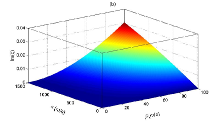
Figure 1: (Color online) The real and imaginary parts of $\xi$ as functions of $\alpha$ and $\beta$. The parameters are chosen as $g=1.52$, $m_{0}=9\times 10^{-31}$ kg, $m=0.15m_{0}$, $B=0.01$T. Under these parameters, we will have $E_{a}/\hbar\approx 1.35$ GHz, $E_{b}/\hbar\approx 1.70$ GHz, and $(|\lambda_{1}/\hbar|,|\lambda_{2}/\hbar|)\approx 5.52\times(\alpha,\beta)$ MHz.

It is obvious that the approximate Hamiltonian $H\mathcal{{}^{\prime}}$ has a similar form as the JC Hamiltonian, and the energy spectrum in the subspace of zero- and one-excitation are obtained as

$$E_{0}^{d} = -\frac{\tilde{E}_{a}}{2}+E,$$ (19)

$$E_{1\pm}^{d} = E+\frac{E_{b}+\tilde{E}_{b}}{2}\pm\sqrt{|\tilde{g}|^{2}+\tilde{\Delta}^{2}},$$ (20)

where

$$\tilde{g} = \frac{\lambda_{1}+\lambda_{2}}{2}-2E_{b}\xi,$$ (21a)

$$E = E_{b}|\xi|^{2}-\frac{\mathrm{Re}[(\lambda_{1}+\lambda_{2})\xi]}{2},$$ (21b)

$$\tilde{\Delta} = \frac{E_{b}+\tilde{E}_{b}-\tilde{E}_{a}}{2}.$$ (21c)

The energy level crossing then occurs when $E_{1-}^{d}=E_{0}^{d}$. In Fig. 2, we plot the energy gap $\Delta E^{d}:=E_{1-}^{d}-E_{0}^{d}$ as a function of $\alpha$ and $\beta$.

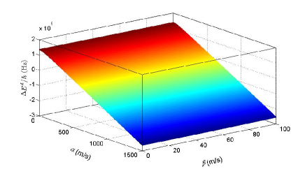
Figure 2: (Color online) The energy gap as a function of $\alpha$ and $\beta$. The parameters are same as those in Fig. 1.

As shown in Fig. 2, for small $\alpha$, $\Delta E^{d}>0$, and the ground state is

$$|G_{1}\rangle = e^{-S}|0;g\rangle$$ (22)

$$= \frac{1}{\sqrt{2}}(|-\xi;+\rangle-|\xi;-\rangle),$$

where $|\pm\rangle$ are the eigen states of Pauli operator $\sigma_{x}$ satisfying $\sigma_{x}|\pm\rangle=\pm|\pm\rangle$, and $|\pm\xi\rangle$ are the bosonic coherent states with amplitudes $\pm\xi$.

As the increase of $\alpha$, the energy level crossing occurs, that is, $\Delta E^{d}$ becomes negative, and the ground state becomes

$$|G_{2}\rangle = e^{-S}[\cos\frac{\theta_{d}}{2}|0;e\rangle-\sin\frac{\theta_{d}}{2}e^{i\phi}|1;g\rangle]$$

$$= e^{-(\xi b^{\dagger}-\xi^{*}b)\sigma_{x}}[\cos\frac{\theta_{d}}{2}|0;e\rangle-\sin\frac{\theta_{d}}{2}e^{i\phi}|1;g\rangle],$$

where

$$\tan\theta_{d}=\frac{|\tilde{g}|}{\tilde{\Delta}},\,\tan\phi=\frac{\mathrm{Im}[\tilde{g}]}{\mathrm{Re}[\tilde{g}]}.$$ (24)

In the end of this section, we would like to emphasize the following point. Besides the quantum well system as discussed in this paper, the anisotropic Rabi model can be realized in various systems, e.g., in the cavity or circuit QED systems. In a typical cavity QED system, in which the atom interacts with the optical cavity mode, the frequencies of the atomic transition and the cavity mode are of the order of $10^{4}-10^{5}$ GHz, and the coupling strength reaches hundreds of MHz AL . In a typical circuit QED system, where the artificial atom (superconducting qubit) couples to the transmission line resonator, the frequencies of the qubit and the resonator are about several GHz, and the coupling strength can be realized by hundreds of MHz IC ; KV . In these two kinds of systems, which motivate many research interests during the past decades, the energy level crossing hardly occurs since the coupling strength is not strong enough. However, the energy level crossing can be available in the realistic quantum well material. Taking the AlAs material as an example, the Lande factor is $g=1.52$, the mass of electron is $m_{0}=9\times 10^{-31}$ kg, and the effective mass is $m=0.15m_{0}$ MV . When the quantum well is subject to a magnetic field $B=0.01$ T in $+z$ direction, we will have $E_{a}/\hbar\approx 1.35$ GHz, $E_{b}/\hbar\approx 1.70$ GHz, and $(|\lambda_{1}|/\hbar,|\lambda_{2}|/\hbar)\approx 5.52\times(\alpha,\beta)$ MHz. When choosing the parameters $\alpha$ in the order of hundreds of m/s and $\beta$ in the order of tens of m/s, which can be achieved easily with recent available experimental techniques loss1 , the coupling strength could be in the same order or even larger than the energies of $E_{a}$ and $E_{b}$. Therefore, the two-dimensional quantum well system provides a promising platform to simulate the energy level crossing behavior and related phenomenon.

IV Quantum Fisher information of the ground state

In the above section, we have depicted the energy level crossing behavior in our system. In this section, the QFI of the ground state is adopted to further characterize the level crossing behavior, and its dependence on $\alpha$ and $\beta$ is detailed studied. We will also give an intuitive explanation about the obtained results based on the stationary perturbation theory.

The so-called quantum Cramér-Rao (CR) inequality, obtained by extending the classical CR inequality to quantum probability and choosing the quantum measurement procedure for any given quantum state to maximize the classical CR inequality, gives a bound to the variance Var$(\hat{\varphi})$ of any unbiased estimator $\hat{\varphi}$ SL ,

$$\text{Var}(\hat{\varphi})\geq\frac{1}{NF_{\varphi}},$$ (25)

where $F_{\varphi}$ is the QFI and $N$ is the number of independent measurements. A larger QFI corresponds to a more accurate estimation to the parameter $\varphi$. Moreover, the QFI is connected to the Bures distance SL through

$$D_{B}^{2}[\rho_{\varphi},\rho_{\varphi+d\varphi}]=\frac{1}{4}F_{\varphi}d\varphi^{2},$$ (26)

where the Bures distance is defined as $D_{B}[\rho,\sigma]:=[2(1-\mathrm{Tr}\sqrt{\rho^{1/2}\sigma\rho^{1/2}})]^{1/2}$.

For an arbitrary given quantum state, its QFI can be determined by the spectrum decomposition of the state. Fortunately, for a pure quantum state given by the wave function $|\psi\rangle$, its QFI with respect to the parameter $\varphi$ has a relatively simple form, given as SL2 ; weizhong ; YMZhang ; Qzheng

$$F_{\varphi}=4(\langle\partial_{\varphi}\psi|\partial_{\varphi}\psi\rangle-|\langle\psi|\partial_{\varphi}\psi\rangle|^{2}).$$ (27)

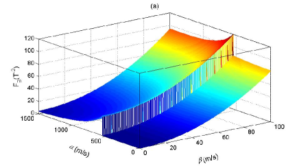
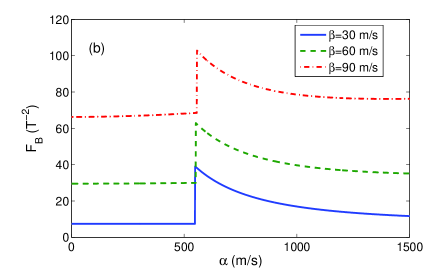
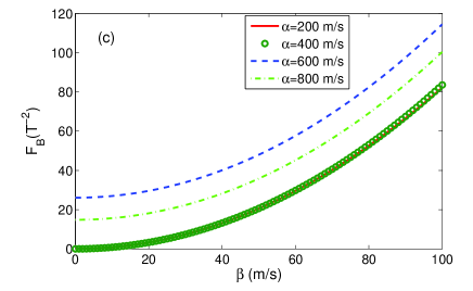
Figure 3: (Color online) (a) The QFI with respect to the external magnetic field $B$, $F_{B}$, as a function of $\alpha$ and $\beta$. (b) $F_{B}$ as a function of $\alpha$ for different $\beta$. (c) $F_{B}$ as a function of $\beta$ for different $\alpha$. The other parameters are the same as those in Fig. 1.

Before the energy level crossing occurs, that is $\Delta E^{d}>0$, the ground state of the system with the presence of both the Rashba and Dresselhaus SOCs is shown in Eq. (22). After some straightforward calculations, its QFI with respect to the external magnetic field $B$ is given as

$$F_{B}=4[(\frac{\partial\mathrm{Re}{\xi}}{\partial B})^{2}+(\frac{\partial\mathrm{Im}{\xi}}{\partial B})^{2}].$$ (28)

After the energy level occurs, that is $\Delta E^{d}<0$, the ground state is given in Eq. (III.2), the expression of the QFI with respective to $B$ is tedious and we will only give the numerical results here.

In Fig. 3(a), we plot the QFI as a function of $\alpha$ and $\beta$. It obviously shows that the QFI undergoes a sudden change when the energy level crossing occurs. Therefore, the QFI of the ground state can be regarded as a witness to the energy level crossing behavior.

Furthermore, in Fig. 3(b), we plot the QFI as a function of $\alpha$ for different values of $\beta$. On one hand, the QFI nearly keeps constant when $\alpha$ approaches the crossing point from small values, and decreases monotonously when $\alpha$ surpasses the crossing value $\alpha^{c}$ ($\alpha^{c}\approx 550$ m/s within our chosen parameters and it corresponds to $|\lambda_{1}^{c}|/\hbar\approx 3$ GHz). On the other hand, a larger $\beta$ will lead to a larger QFI, which implies a more precise measurement about the magnetic field. This result is also demonstrated in Fig. 3(c), where the QFI is plotted as a function of $\beta$ for different values of $\alpha$. It shows that the curves for $\alpha=200$ m/s and $\alpha=400$ m/s, which are both below the crossing values, coincide with each other. As for the values above the crossing point, we observe a decreasing behavior of QFI as the increase of $\alpha$, for example, the QFI for $\alpha=600$ m/s is larger than that for $\alpha=800$ m/s as shown in Fig. 3(c).

The dependence of QFI on the strengths of the Rashba and Dresselhaus SOCs can be explained from the viewpoint of the stationary perturbation theory qualitatively as what follows. In our consideration, the strength of Dresselhaus SOC is much weaker than that of the Rashba SOC and the bare energy of spin/orbit degree of the freedom, so it can be regarded as a perturbation. In this sense, the mapped Hamiltonian [Eq. (5)] can be divided into $H=H_{0}+H_{I}$, where the un-perturbation part is

$$H_{0}=E_{b}b^{\dagger}b+\frac{E_{a}}{2}\sigma_{z}+(\frac{\lambda_{1}}{2}b^{\dagger}\sigma_{-}+\frac{\lambda_{1}^{\ast}}{2}\sigma_{+}b),$$ (29)

and the perturbation part is

$$H_{I}=(\frac{\lambda_{2}}{2}b\sigma_{-}+\frac{\lambda_{2}^{\ast}}{2}\sigma_{+}b^{\dagger}).$$ (30)

For small $\alpha$ or $|\lambda_{1}|$, the ground state of $H_{0}$ is $|0;g\rangle$ which is independent of the field $B$ and yields a zero QFI. The perturbation part, which is contributed from the Dresselhaus SOC, mixes the state $|0;g\rangle$ with $|1;e\rangle$, yields an entangled ground state and gives a non-zero $\beta$ ($|\lambda_{2}|$) dependent QFI. It is obvious that the Dresselhaus SOC will enhance the entanglement, so that the QFI also increases as $\beta$ becomes larger.

For large $\alpha$ or $|\lambda_{1}|$, the energy level crossing occurs, and the ground state of $H_{0}$ becomes the wave function given in Eq. (8), which is an entangled state, yields a non-zero QFI. Furthermore, the entanglement decreases (increases) with the increase of $\alpha$ ($\beta$), and so the QFI behaves in a similar way.

V Conclusion

In this paper, we investigate the energy level crossing behavior and the QFI of the ground state in the AlAs semiconductor quantum well. The Hamiltonian of the system with the Rashba and Dresselhaus SOCs simultaneously is mapped onto an anisotropic Rabi model in quantum optics. We find that although the mapped Hamiltonian is similar to that in cavity and circuit QED systems, the energy level crossing behavior only occurs in our current system with the available parameters. As a probe of the energy level crossing in our system, we discuss the QFI of the ground state and find that the QFI exhibits different dependences on the strengths of the Rashba and Dresselhaus SOCs and has a sudden jump when the crossing happens. Based on the stationary perturbation theory, we give an intuitive explanation to the results.

- (1) S. Nadj-Perge, S. M. Frolov, E. P. A. M. Bakkers, and L. P. Kouwenhoven, Nature (London) 468, 1084 (2010).
- (2) R. Li, J. Q. You, C. P. Sun, and F. Nori, Phys. Rev. Lett. 111, 086805 (2013).
- (3) I. Zutic, J. Fabian, and S. Das Sarma, Rev. Mod. Phys. 76, 323 (2004).
- (4) D. D. Awschalom, N. Samarth, and D. Loss, Semiconductor Spintronics and Quantum Computation (Springer-Verlag, Berlin, 2002).
- (5) E. I. Rashba, Fiz. Tverd. Tela (Leningrad) 2, 1224 (1960) [Sov. Phys. Solid State 2, 1109 (1960)]; Y. A. Bychkov and E. I. Rashba, J. Phys. C 17, 6039 (1984).
- (6) G. Dresselhaus, Phys. Rev. 100, 580 (1955).
- (7) O. Voskoboynikov, C. P. Lee, and O. Tretyak, Phys. Rev. B 63, 165306 (2001).
- (8) J. Schiemann, J. C. Egues, and D. Loss, Phys. Rev. B 67, 085302 (2003).
- (9) S. Debald and C. Emary, Phys. Rev. Lett. 94, 226803 (2005).
- (10) Q.-T. Xie, S. Cui, J.-P. Cao, L. Amico, and H. Fan, Phys. Rev. X 4, 021046 (2014).
- (11) R. H. Dicke, Phys. Rev. 93, 99 (1954).
- (12) D. Nagy, G. Konya, G. Szirmai, and P. Domokos, Phys. Rev. Lett. 104, 130401 (2010).
- (13) T.-L. Wang, L.-N. Wu, W. Yang, G.-R. Jin, N. Lambert, and F. Nori, New J. Phys. 16, 063039 (2014).
- (14) Y. Yao, L. Ge, X. Xiao, X. G. Wang, and C. P. Sun, Phys. Rev. A 90, 022327 (2014); H. Song, S. Luo, N. Li, and L. Chang, Phys. Rev. A 88, 042121 (2013).
- (15) A. Smerzi, Phys. Rev. Lett. 109, 150410 (2012).
- (16) L. Pezze and A. Smerzi, Phys. Rev. Lett. 102, 100401 (2009).
- (17) N. Li and S. Luo, Phys. Rev. A 88, 014301 (2013).
- (18) E. I. Rashba, Physica E 20, 189 (2004).
- (19) L.-T. Shen, Z.-B. Yang, M. Lu, R.-X. Chen, and H.-Z. Wu, Applied Physics B 117, 195 (2014).
- (20) G. Zhang and H. Zhu, Sci. Rep. 5, 8756 (2015).
- (21) Y. Wang and J. Y. Haw, Phys. Lett. A 379, 779 (2015).
- (22) A. Baksic and C. Cuiti, Phys. Rev. Lett. 112, 173601 (2014).
- (23) N. Zhao, L. Zhong, J.-L. Zhu, and C. P. Sun, Phys. Rev. B 74, 075307 (2006).
- (24) S. Ashhab, Phys. Rev. A 87, 013826 (2013).
- (25) D. V. Bulaev and D. Loss, Phys. Rev. B 71, 205324 (2005).
- (26) D. Braak, Phys. Rev. Lett. 107, 100401 (2011).
- (27) Z. G. Lü and H. Zheng, Phys. Rev. B 75, 054302 (2007).
- (28) G. J. Gan and H. Zheng, Eur. Phys. J. D 59, 473 (2010).
- (29) Q. Ai, Y. Li, H. Zheng, and C. P. Sun, Phys. Rev. A 81, 042116 (2010).
- (30) A. L. Grimsmo and S. Parkins, Phys. Rev. A 87, 033814 (2013).
- (31) I. Chiorescu, P. Bertet, K. Semba, Y. Nakamura, C. J. P. M. Harmans, and J. E. Mooij, Nature (London) 431, 159 (2004).
- (32) K. V. R. M. Murali, Z. Dutton, W. Oliver, D. Crankshaw, and T. Orlando, Phys. Rev. Lett. 93, 087003 (2004).
- (33) M. V. Rodriguez and R. G. Nazmitdinov, Phys. Rev. B 73, 235306 (2006).
- (34) S. L. Braunstein and C. M. Caves, Phys. Rev. Lett. 72, 3439 (1994).
- (35) S. L. Braunstein, C. M. Caves, and G. J. Milburn, Ann. Phys. (N.Y.) 247, 135 (1996).
- (36) W. Zhong, Zhe Sun, J. Ma, X. Wang, and F. Nori, Phys. Rev. A 87, 022337 (2013).
- (37) Y. M. Zhang, X. W. Li, W. Yang, and G. R. Jin, Phys. Rev. A 88, 043832 (2013).
- (38) Q. Zheng, L. Ge, Y. Yao, and Q.-j. Zhi, Phys. Rev. A 91, 033805 (2015).