Measurement of spin-flip probabilities for ultracold neutrons interacting with nickel phosphorus coated surfaces

Abstract

We report a measurement of the spin-flip probabilities for ultracold neutrons interacting with surfaces coated with nickel phosphorus. For 50 $\mu$m thick nickel phosphorus coated on stainless steel, the spin-flip probability per bounce was found to be $\beta_{\rm NiP\;on\;SS}=(3.3^{+1.8}_{-5.6})\times 10^{-6}$. For 50 $\mu$m thick nickel phosphorus coated on aluminum, the spin-flip probability per bounce was found to be $\beta_{\rm NiP\;on\;Al}=(3.6^{+2.1}_{-5.9})\times 10^{-6}$. For the copper guide used as reference, the spin flip probability per bounce was found to be $\beta_{\rm Cu}=(6.7^{+5.0}_{-2.5})\times 10^{-6}$. The results on the nickel phosphorus-coated surfaces may be interpreted as upper limits, yielding $\beta_{\rm NiP\;on\;SS}<6.2\times 10^{-6}$ (90% C.L.) and $\beta_{\rm NiP\;on\;Al}<7.0\times 10^{-6}$ (90% C.L.) for 50 $\mu$m thick nickel phosphorus coated on stainless steel and 50 $\mu$m thick nickel phosphorus coated on aluminum, respectively. Nickel phosphorus coated stainless steel or aluminum provides a solution when low-cost, mechanically robust, and non-depolarizing UCN guides with a high-Fermi-potential are needed.

1 Introduction

Ultracold neutrons (UCNs) are defined operationally to be neutrons of sufficiently low kinetic energies that they can be confined in a material bottle, corresponding to kinetic energies below about 340 neV. UCNs are playing increasingly important roles in the studies of fundamental physical interactions (for recent reviews, see e.g. Refs. [1, 2]).

Experiments using UCNs are being performed at UCN facilities around the world, including Institut Laue-Langevin (ILL) [3], Los Alamos National Laboratory (LANL) [4], Research Center for Nuclear Physics (RCNP) at Osaka University [5], Paul Scherrer Institut (PSI) [6], and University of Mainz [7]. One important component for experiments at such facilities is the UCN transport guides. These guides are used to transport UCNs from a source to experiments and from one part of an experiment to another. For applications that require spin polarized UCNs, it is important that UCNs retain their polarization as they are transported (see e.g. Ref. [8]).

In other applications in which polarized UCNs are stored for extended periods of time, such as neutron electric dipole moment experiments (see e.g. Ref. [9]) and the UCNA experiment (see e.g. Ref. [10]), it is also important that UCNs remain highly polarized while they are stored in a material bottle. In some cases, the depolarization of UCNs due to wall collisions is one of the dominant sources of systematic uncertainties in the final result of the experiment [11].

Because of its importance for these applications, the study of spin-flip probabilities and the possible mechanisms for spin flip is an active area of research [12, 13, 14, 15]. The spin-flip probability per bounce has been measured for various materials. References [12, 14] report results on beryllium, quartz, beryllium oxide, glass, graphite, brass, copper, and Teflon, whereas Ref. [15] discusses results on diamond-like carbon (DLC) coated on aluminum foil and on polyethylene terephthalate (PET) foil. In addition, measurements of the spin-flip probability per bounce have been performed for DLC-coated quartz [16], stainless steel, electropolished copper, and DLC-coated copper [17]. (The results from Ref. [17] are available in Ref. [18].) The reported values for the spin-flip probability per bounce are on the order of $10^{-6}-10^{-5}$ for all of these materials with the exception of stainless steel, for which a reported preliminary value for the spin-flip probability per bounce is on the order of $10^{-3}$ [17], two to three orders of magnitude larger.

The spin-flipping elastic or quasielastic incoherent scattering from protons in surface hydrogen contamination has been considered to be a possible mechanism for UCN spin flip upon interaction with a surface [12, 13, 14, 15]. So far, however, data and model calculations have not been in agreement.

Another possible mechanism is Majorana spin flip [19] due to magnetic field inhomogeneity near material surfaces, from ferromagnetic impurities or magnetization of the material itself. In addition, the sudden change in direction that occurs when a UCN reflects from a surface can cause a spin flip in the presence of moderate gradients [13]. Gamblin and Carver [20] discuss such an effect for ³He atoms. The high spin-flip probability observed for stainless steel in a large holding field [17] is likely due to magnetic field inhomogeneity near material surfaces or magnetization of the material itself.

Recently, based on the suggestion from Ref. [21], we have identified nickel phosphorus (NiP) coating to be a promising UCN coating material with a small loss per bounce and a high Fermi potential [22]. The Fermi potentials of NiP samples with a phosphorus content of 10.5 wt.% (18.2 at.%) coated on stainless steel and on aluminum were both found to be $\approx$213 neV [22], which is consistent with the calculated value and is to be compared to 188 neV for stainless steel and 168 neV for copper. NiP coating is extremely robust and is widely used in industrial applications. It is highly attractive from a practical point of view because the coating can be applied commercially in a rather straightforward chemical process, and there are numerous vendors that can provide such a service economically. It is important that the coating process not use neutron absorbing materials such as cadmium. Furthermore, alloying nickel with phosphorus lowers its Curie temperature (see e.g. Refs. [23, 24, 25]). As a result, when made with high enough phosphorus content, NiP is known to be non-magnetic at room temperature. Therefore, it is of great interest to study its UCN spin depolarization properties and how depolarization depends on the material used for the substrate.

In this paper, we report a measurement of the spin-flip probabilities for UCNs interacting with NiP-coated surfaces. We investigated aluminum and stainless steel as the substrate. The results obtained with NiP-coated surfaces are compared to those obtained with copper guides. This measurement was performed as part of development work for a new neutron electric dipole moment experiment at the LANL UCN facility [26] and an associated UCN source upgrade [27].

This paper is organized as follows. In Sec. 2, the experimental apparatus and method are described. Section 3 describes the analysis of the data. In Sec. 4, we discuss the implication of the results on future experiments using UCNs. Section 5 provides a short summary of the content of this paper.

2 Experiment

2.1 Apparatus and method

The measurement was performed at the LANL UCN facility [4]. Spallation neutrons produced by a pulsed 800-MeV proton beam striking a tungsten target were moderated by beryllium and graphite moderators at ambient temperature and further cooled by a cold moderator that consisted of cooled polyethylene beads. The cold neutrons were converted to UCNs by a solid deuterium (SD₂) converter. UCNs were directed upward 1 m along a vertical guide coated with ⁵⁸Ni and then 6 m along a horizontal guide made of stainless steel before exiting the biological shield. At the bottom of the vertical UCN guide was a butterfly valve that remained closed when there was no proton beam pulse striking the spallation target in order to keep the UCNs from returning to the SD₂ where they would be absorbed.

A schematic diagram of the experimental setup for the depolarization measurement is shown in Fig. 1.

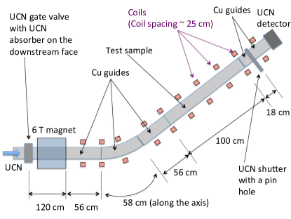
Figure 1: Schematic diagram of the experimental setup

When the UCN gate valve was opened, UCNs transported from the source entered the apparatus. UCNs in one spin state, the so-called “high-field seekers” for which $\bm{\mu}\cdot\bm{B}<0$ where $\bm{\mu}$ is the magnetic dipole moment of the neutron and $\bm{B}$ is a magnetic field, were able to move past the 6 T magnetic field provided by a superconducting solenoidal magnet. UCNs in the other spin state, the so-called “low-field seekers”, were reflected back by the potential barrier due to $\bm{\mu}\cdot\bm{B}>0$. For $|\bm{B}|=6$ T, $|\bm{\mu}\cdot\bm{B}|=360$ neV, much larger than the kinetic energy of the neutrons from the LANL UCN source, which has a cutoff at $\approx$190 neV.

On the other side of the high-field region was a UCN guide system (76.2 mm in OD, 72.9 mm in ID) that consisted of a set of copper guide sections, a NiP-coated guide section, a section of a copper guide with a UCN shutter, and a short section of a copper guide followed by a UCN detector [28]. The guides were placed in a $\sim$2 mT magnetic field provided by a set of coils in order to retain the polarization of the UCNs. The UCN shutter, made of copper, had a pinhole 5 mm in diameter. The gap between the UCN shutter and the end of the guide leading to it was measured to be $\sim$0.05 mm.

The high-field seekers were able to move freely through the high magnetic field region, colliding with the inner walls of the guide system. The number of collisions per second for the high-field seekers in the guide system downstream of the 6 T field region is given by

$$R_{\rm hfs}=\frac{1}{4}A_{\rm tot}\,\langle v_{\rm hfs}\rangle\,n_{\rm hfs},$$ (1)

where $A_{\rm tot}$ is the total inner surface of the system that the high field seekers interacted with in the guide system downstream of the 6 T field region, $\langle v_{\rm hfs}\rangle$ is the average velocity of the high-field seekers, and $n_{\rm hfs}$ is the density of the high-field seekers. The rate of collisions for the high field seekers was monitored during this time by detecting neutrons that leaked through a pinhole on the shutter in the downstream end of the test guide assembly. If UCNs are detected at a rate of $R_{\rm h}$ and the area of the pinhole is $A_{\rm h}$, $R_{\rm hfs}$ can be inferred to be

$$R_{\rm hfs}=\frac{A_{\rm tot}}{A_{\rm h}}R_{\rm h},$$ (2)

assuming that the distribution of UCNs inside the system is uniform and isotropic. We discuss the validity of this assumption in Sec. 3. For our geometry, ${A_{\rm tot}}/{A_{\rm h}}=3.36\times 10^{4}$.

While the high-field seekers collided with the inner wall of the system at the rate of $R_{\rm hfs}$, spin-flipped neutrons were produced at a rate of

$$R_{\rm dep}=R_{\rm hfs}\,\beta=\frac{A_{\rm tot}}{A_{\rm h}}R_{\rm h}\,\beta,$$ (3)

where $\beta$ is the probability of spin flip per bounce. While in principle $\beta$ can depend on the neutron velocity as well as the angle of incidence, and such dependencies can give important information on the possible mechanism of UCN depolarization upon wall collision, we assumed $\beta$ to be independent of the velocity and angle of incidence in our analysis. Reference [15] observed no indication of energy dependence within the accuracy of their measurement for the depolarization per bounce on DLC.

The spin-flipped neutrons were not able to pass through the 6 T field region and hence became “trapped” in the guide assembly downstream of the 6 T field region. The number of trapped spin-flipped neutrons in the system at time $t$, $n_{\rm dep}(t)$, satisfies the following differential equation:

$$\frac{dn_{\rm dep}(t)}{dt}=\beta\frac{A_{\rm tot}}{A_{\rm h}}R_{\rm h}(t)-\frac{1}{\tau_{\rm dep}}n_{\rm dep}(t),$$ (4)

where $\tau_{\rm dep}$ is the lifetime of the spin-flipped neutrons. If $R_{\rm hfs}$ was constant, then the number of the spin-flipped low-field seekers built up as $[1-\exp(-t/\tau_{\rm dep})]$. In general, $\tau_{\rm dep}$ depends on the UCN velocity $v$. With the velocity dependence taken into account, Eq. (4) becomes

$$\frac{\partial^{2}n_{\rm dep}}{\partial v\,\partial t}=\beta\frac{A_{\rm tot}}{A_{\rm h}}P(v,t)R_{\rm h}(t)-\frac{1}{\tau_{\rm dep}(v)}\frac{\partial n_{\rm dep}}{\partial v},$$ (5)

where $P(v,t)$ is the normalized velocity distribution of UCNs at the time of spin flip, and $\int_{0}^{v_{c}}\frac{\partial n_{\rm dep}}{\partial v}dv=n_{\rm dep}$ where $v_{\rm c}$ is the cutoff velocity.

The UCN gate valve upstream of the 6 T region was then closed, after which time the high-field seekers were quickly absorbed by a thin sheet of polymethylpentene (TPX) attached to the downstream side of the gate valve. On the other hand, the spin-flipped low-field seekers remained trapped in the volume between the 6 T field and the UCN shutter. Opening the shutter allowed the trapped spin-flipped UCNs to be rapidly drained from the guide system into the detector.

If the UCN gate valve initially remained open for loading time $T_{\rm L}$ , followed by cleaning time $T_{\rm C}$ during which time both the UCN gate valve and the UCN shutter remained closed and at the end of which the UCN shutter was opened, the number of the detected spin-flipped neutrons is given by integrating Eq. (5):

$$N_{\rm dep}=\beta\frac{A_{\rm tot}}{A_{\rm h}}\int_{0}^{T_{\rm L}+T_{\rm C}}\int_{0}^{v_{\rm c}}P(v,t)R_{\rm h}(t)e^{-\frac{T_{\rm L}+T_{\rm C}-t}{\tau_{\rm dep}(v)}}dv\,dt,$$ (6)

where $N_{\rm dep}=n_{\rm dep}(t)$ at $t=T_{\rm L}+T_{\rm C}$. Since both the high-field seekers and the spin-flipped low-field seekers are detected by the same UCN detector, the possible finite detection efficiency cancels in Eqs. (4), (5), and (6). Measuring $N_{\rm dep}$ and $R_{\rm h}(t)$, with sufficient knowledge of $P(v,t)$ and $\tau_{\rm dep}(v)$, determines $\beta$.

The currents for the coils providing the holding field were adjusted so that the field was higher than 2 mT and the gradient was smaller than 10 mT/cm to ensure that the probability of Majorana spin flip due to UCN passing an inhomogeneous field region or due to wall collision in an inhomogeneous field was less than $10^{-6}$ per pass or per bounce [19].

As seen in Fig. 1 and Table 1, a large portion of the guide system downstream of the 6 T field was made of copper. Copper was chosen because its spin-flip probability was determined to be low by previous measurements [12, 14]. The surface area of the test sample was $\sim$35% of the total surface area of the guide system, diluting the sensitivity to the spin flip due to the test sample. This was due to geometrical constraints in the experimental area.

2.2 Sample preparation

Two NiP-coated samples were prepared, one on a 316L stainless steel tube and the other on an aluminum tube. Both tubes had an ID of 72.9 mm. The 316L stainless steel tube was cut from welded tubing that had been polished and electropolished to roughness average (Ra) of 10 microinches (0.254 $\mu$m), purchased from Valex (specification 401) [29]. The aluminum tube was cut from unpolished 6061-T6511 aluminum tubing.

The coating was applied using high-phosphorus content electroless nickel phosphorus plating. Electroless nickel plating is an autocatalytic process in which the deposition of nickel is brought by chemical reduction of a nickel salt with a reducing agent [30, 31]. Electroless NiP deposits exhibit numerous advantages over those done by other methods [31]. The advantages include hardness, corrosion and wear resistance, plating thickness uniformity, and adjustable magnetic and electrical properties. Because of these advantages, the electroless plating method is widely used in industry. The coating of our samples was done by Chem Processing, Inc. [32]. The phosphorus content was $10.5\pm 0.25$ wt.% ($18.2\pm 0.4$ at.%). The thickness of the coating was 50 $\mu$m, the largest thickness provided by the vendor, for both samples. We made this choice as we were interested in seeing if this coating material could keep UCNs from seeing the stainless steel’s magnetic surface. (We prepared samples with thinner coating but the limited beam time available to us did not allow us to make measurements with them.) Post-baking at 375$\degree$C for 20 hours was performed for both samples to increase the hardness. Baking also has the effect of removing hydrogen from the NiP coating [33]. The coated surface was then cleaned with the following procedure:

1. The samples were submerged in Alconox solution (1 wt.%) at 60^∘C for 10 hours.

2. The samples were then rinsed with deionized water and then with isopropyl alcohol.

2.3 Measurement

Measurements were performed for both NiP-coated guide samples. In addition, to measure the contributions from the rest of the system including the copper guides and the shutter, measurements were made with the NiP samples removed. (The limited beam time did not allow us to perform measurements on uncoated stainless steel samples.) A description of the three configurations for which measurements were made is listed in Table 1. For all configurations, two series of measurements were performed: one in which $T_{\rm C}$ was fixed and $T_{\rm L}$ was varied (loading time scan) and another in which $T_{\rm L}$ was fixed and $T_{\rm C}$ was varied (cleaning time scan). Table 2 lists the values of $T_{\rm C}$ and $T_{\rm L}$ used in the measurements, and Fig. 2 shows an example of the measured neutron count rate as a function of time.

Table 1: Description of the three configurations for which measurements were performed.

Configuration	Description	Cu guide length	NiP guide length
C1	SS guide with 50 $\mu$m NiP coating	188 cm	100 cm
C2	Al guide with 50 $\mu$m NiP coating	188 cm	100 cm
C3	No NiP-coated guide	188 cm	0 cm

Table 2: The values of $T_{\rm C}$ and $T_{\rm L}$ used for the loading-time and the cleaning-time scans.

Scan	$T_{\rm L}$ (s)	$T_{\rm C}$ (s)
Loading time scan	10, 20, 40, 60, 80 (C1 only)	60
Cleaning time scan	20 (C2), 50 (C1, C3)	20, 40, 60, 80

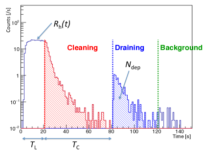
Figure 2: Neutron count rate as a function of time obtained for configuration C2 for $T_{\rm L}=20$ s and $T_{\rm C}=60$ s.

3 Data Analysis

As mentioned earlier, Eq. (6) allows determination of $\beta$ from experimentally measured $R_{\rm h}(t)$ and $N_{\rm dep}$ if $P(v,t)$ and $\tau_{\rm dep}(v)$ are known with sufficient accuracy. $P(v,t)$ depends not only on the velocity distribution of the UCN entering the system but also on the lifetime of high-field seekers in the system $\tau_{\rm hfs}(v)$. In turn, $\tau_{\rm hfs}(v)$, as well as $\tau_{\rm dep}(v)$, depends not only on the surface-UCN interactions but also on how the system was assembled, as for many systems the UCN loss is dominated by gaps at joints between UCN guide sections.

Equation (6) assumes [through Eq. (2)] that the distribution of UCNs inside the system was uniform and isotropic. This assumption is justified as follows. Firstly, the $1/e$ time to drain the system was measured to be $\sim$3 s for C1 and C2, and $\sim$2 s for C3, by fitting the “Cleaning” part of the neutron time spectra (such as the one shown in Fig. 2). This indicates that the system reached a uniform density within 2 to 3 s, a time scale much shorter than the loading time. Secondly, the transport properties of the UCN guides that we use are typically well described with Monte Carlo simulations when we use a nonspecularity of $\epsilon\sim 0.03$ or higher with the Lambertian angular distributions for nonspecular reflection [34]. Since the mean free path between collisions in a tube of radius $R$ is $2R$, UCNs undergo nonspecular reflection approximately every $2R/(v\,\epsilon)\sim 0.6$ s. This indicates that UCNs in the system reached an isotropic distribution in a time period much smaller than the loading time.

In the absence of sufficiently accurate experimentally obtained information on $P(v,t)$ and $\tau_{\rm dep}$, we resorted to analysis models in which approximations were made to Eq. (6) and evaluated the effect of those approximations to the extracted values of $\beta$. Below we describe the two specific analysis models we employed and the results obtained from them.

3.1 Analysis model 1

In this model, $\tau_{\rm dep}$ is assumed to be independent of neutron velocity $v$. With this assumption, Eq. (6) simplifies to

$$N_{\rm dep}=\beta\frac{A_{\rm tot}}{A_{\rm h}}\int_{0}^{T_{\rm L}+T_{\rm C}}R_{\rm h}(t)\,e^{-\frac{T_{\rm L}+T_{\rm C}-t}{\tau_{\rm dep}}}dt.$$ (7)

From the experimentally measured $R_{\rm h}(t)$ and $N_{\rm dep}$, we obtained the values of $\beta$ for a set of assumed values for $\tau_{\rm dep}$. For the correct value of $\tau_{\rm dep}$, $\beta$ should be independent of $T_{\rm L}$ and $T_{\rm C}$. Figure 3 shows plots of $\beta$ for a set of values of $\tau_{\rm dep}$ for both the $T_{\rm L}$ and $T_{\rm C}$ scans.

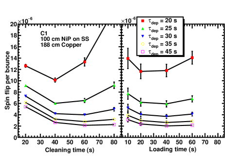
Figure 3: Plots of $\beta$ for a set of values of $\tau_{\rm dep}$ for both the $T_{\rm L}$ and $T_{\rm C}$ scans obtained assuming Eq. (7). The error bar on each point represent the statistical uncertainty, which is dominated by the counting statistics of $N_{\rm dep}$.

In this analysis, $N_{\rm dep}$ was determined by counting UCNs over a period of 40 s after $t=T_{\rm L}+T_{c}$ and subtracting the background estimated from the counts after the counting period.

From these results we see the following:

• $\beta\sim 4\times 10^{-6}$ can describe data for all combinations of $T_{\rm L}$ and $T_{\rm C}$ for all three configurations reasonably well except for $T_{\rm C}=20$ s.

• The deviation for $T_{\rm C}=20$ s is larger for configurations C1 and C2 than for configuration C3.

The deviation of the data points for $T_{\rm C}=20$ s from other data points can be attributed to the fact that 20 s was not sufficiently long to remove all the high-field seekers, and as a result there were high-field seekers included in what was counted as $N_{\rm dep}$. That $T_{\rm C}$ of 20 s was not sufficient to remove all the high-field seekers can be clearly seen in Fig. 2.

The “best fit” values of $\beta$ and $\tau_{\rm dep}$ can be obtained by minimizing $\chi^{2}$ defined as

$$\chi^{2}=\sum_{i=\{T_{\rm C},T_{\rm L}\}}\frac{\{\beta_{i}(\tau_{\rm dep})-\beta\}^{2}}{(\delta\beta_{i})^{2}},$$ (8)

where the summation is over all combinations of $\{T_{\rm C},T_{\rm L}\}$ except for $T_{\rm C}=20$ s. The obtained best fit values of $\beta$ and $\tau_{\rm dep}$ as well as the 1 $\sigma$ boundary are graphically indicated in Fig. 4 for each configuration. The numerical results are listed in Table 3.

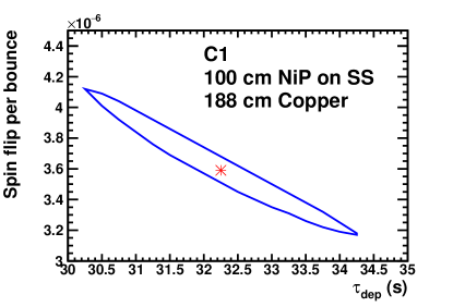
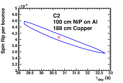
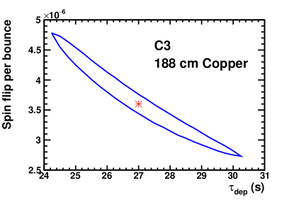
Figure 4: best fit values of $\beta$ and $\tau_{\rm dep}$ as well as the 1 $\sigma$ boundary for each configuration for analysis model 1.

Table 3: Results obtained from Analysis Model 1. Only the best fit values are listed for $\tau_{\rm dep}$. For description of the guide configurations, see Table 1.

Guide	$\beta$	$\tau_{\rm dep}$ (s)	$\chi^{2}$/DOF
C1	$(3.6^{+0.5}_{-0.4})\times 10^{-6}$	32.3	1.49
C2	$(4.1^{+0.5}_{-0.5})\times 10^{-6}$	30.3	0.94
C3	$(3.6^{+1.2}_{-0.9})\times 10^{-6}$	27.0	0.84

3.2 Analysis model 2

In this model, we assumed $P(v)\propto v^{2}$. The $v^{2}$ dependence is well motivated from Monte Carlo simulations performed on the UCN production and transport [34]. For the UCN loss, we assumed

$$\tau_{\rm dep}(v)=\left(\frac{v}{4}\frac{A_{\rm tot}}{V}f\right)^{-1},$$ (9)

where $V$ is the volume of the trap and $f$ is a factor corresponding to the probability of UCN loss per collision. In this model we assumed $f$ to be independent of the UCN energy and the angle of incidence. This is a good approximation when UCN loss is dominated by gaps in the system, and not by the interaction of UCNs with walls, as is the case for this system as discussed in Sec. 3.3.

Substituting Eq. (9) into Eq. (6) with a model $P(v)=\frac{3}{v_{\rm c}^{3}}v^{2}$ and integrating over $v$ yields

$$N_{\rm dep} = \beta\frac{A_{\rm tot}}{A_{\rm h}}\frac{3}{v_{\rm c}^{3}}\int_{0}^{T_{\rm L}+T_{\rm C}}dt\,R_{\rm h}(t)$$ (10)

$$\times \frac{2+e^{-a\,v_{\rm c}}\left\{-2-a\,v_{\rm c}\left(2+a\,v_{\rm c}\right)\right\}}{a^{3}},$$

where $a=\frac{1}{4}\frac{A_{\rm tot}}{V}f\,(T_{\rm L}+T_{\rm C}-t)$.

From the experimentally measured $R_{\rm h}(t)$ and $N_{\rm dep}$, we obtained the values $\beta$ for a set of assumed values of $f$ using Eq. (10) with $v_{\rm c}=5.66$ m/s corresponding to the cutoff energy for copper. The “best fit” values of $\beta$ and $\tau_{\rm dep}$ were obtained by minimizing $\chi^{2}$ defined as

$$\chi^{2}=\sum_{i=\{T_{\rm C},T_{\rm L}\}}\frac{\{\beta_{i}(f)-\beta\}^{2}}{(\delta\beta_{i})^{2}},$$ (11)

where the summation is over all combinations of $\{T_{\rm C},T_{\rm L}\}$ except for $T_{\rm C}=20$ s. The obtained best fit values of $\beta$ and $f$ as well as the 1 $\sigma$ boundary are graphically indicated in Fig. 5 for each configuration. The numerical results are listed in Table 4.

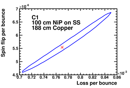
Figure 5: best fit values of $\beta$ and $\tau_{\rm dep}$ as well as the 1 $\sigma$ boundary for each configuration for analysis model 2.

Table 4: Results obtained from Analysis Model 2. Only the best fit values are listed for $f$. For description of the guide configurations, see Table 1.

Guide	$\beta$	$f$	$\chi^{2}$/DOF
C1	$(5.5^{+1.3}_{-1.0})\times 10^{-6}$	$7.7\times 10^{-4}$	0.99
C2	$(5.6^{+1.2}_{-0.9})\times 10^{-6}$	$7.7\times 10^{-4}$	0.97
C3	$(6.7^{+5.0}_{-2.5})\times 10^{-6}$	$1.0\times 10^{-3}$	0.99

3.3 Discussion of the analysis results

While the two analysis methods yielded somewhat different values for $\beta$, in each analysis, the difference in $\beta$ among different guide configurations were small, indicating that the NiP-coated guide sections were as non-depolarizing as copper guides.

Now we discuss possible systematic biases introduced in the results due to the simplifying assumptions made for each of the analysis models. In Analysis Model 1, it was assumed that the lifetime of the depolarized neutrons was the same regardless of the UCN velocity. It is usually the case that slower neutrons have a longer lifetime, because the loss rate is proportional to the rate of collision with the walls and also the loss per bounce is larger for faster neutrons. This effect causes the average velocity of UCNs trapped for an extended period of time to be lower than the initial average velocity. Thus the assumption of velocity independent UCN lifetime ignores the possible spectral difference between the high-field seekers that initially occupied the system and the detected spin-flipped UCNs. Since the detected spin-flipped UCNs tended to have lower velocities than the initial high-field seekers, the estimation of the collision rate using the measured $R_{\rm h}$ is an overestimate for the detected spin-flipped UCNs. This results in an underestimate of the spin flip probability $\beta$.

Analysis Model 2 addresses this problem. It describes UCN loss with a single parameter, the loss per bounce $f$, which is independent of the UCN velocity. As mentioned earlier, this is a good approximation when the UCN loss is dominated by gaps in the system. In fact, the obtained values of $f$ are $\sim$10^-3, much larger than the typical loss per bounce due to collision with material walls. Here, $f\sim 10^{-3}$ indicates a 1 mm wide gap for every 1 m of guide, which agrees with previous assessments of gaps in typical guide assemblies of this type. The contribution to $f$ from the pinhole is much smaller, $\approx 2.9\times 10^{-5}$ for C1 and C2 and $\approx 1.3\times 10^{-5}$ for C3.

The values of $\beta$ obtained from Analysis Model 2 are larger than those from Analysis 1 by a factor of 1.4-1.9. This can be explained by the underestimation of $\beta$ in Analysis Model 1 that was discussed earlier. The size of this effect can be estimated as follows. For a neutron velocity spectrum proportional to $v^{2}$, the average velocity is $v_{\rm ave}=\frac{3}{4}v_{\rm c}$. If the UCN loss is described by a constant loss per bounce $f$, then the average velocity of the UCN after time $t$ is

$$v_{\rm ave}(t) = \frac{\int_{0}^{v_{\rm c}}v^{3}e^{-b\,v\,t}\,dv}{\int_{0}^{v_{\rm c}}v^{2}e^{-b\,v\,t}\,dv}$$ (12)

$$= \frac{6+e^{-c}[-6-c\,\{6+c\,(3+c)\}]}{b\,t\,[2+e^{-c}\{-2-c\,(2+c)\}]},$$

where $b=\frac{1}{4}\frac{A_{\rm tot}}{V}f$ and $c=b\,t\,v_{\rm c}$. Inserting the values from this experiment of $v_{\rm c}=5.66$ m/s, $4V/A_{\rm tot}=7.62$ cm, and $f=0.7\times 10^{-3}$ gives $\frac{v_{\rm ave}(t)}{v_{\rm ave}(0)}\simeq 1.5$ for e.g. $t=100$ s, consistent with the observation made with the comparison between Analysis Models 1 and 2.

Both analysis results indicate that the UCN loss was smaller when a NiP-coated guide section was included in the system than it was when the system was solely made of copper guides. This can be attributed to two factors: (1) the smaller average number of gaps per unit length when the NiP-coated guide is included in the system as the NiP-coated section is longer than the other guide section (see Fig. 1), and (2) the superior UCN storage properties of NiP-coated guides that we observed [22], which is due to the higher Fermi potential of NiP.

Assuming that UCNs were uniformly distributed inside the system we can relate the spin flip probabilities obtained for the three configurations to separate contributions from NiP-coated and copper surfaces:

$$\beta_{\rm C1,C2}=f_{\rm Cu}\,\beta_{\rm Cu}+f_{\rm NiP}\,\beta_{\rm NiP},$$ (13)

where $f_{\rm Cu}$ and $f_{\rm NiP}$ are the fraction of the copper surface and that of the NiP-coated surface in the system with $f_{\rm NiP}=0.35$ and $f_{\rm Cu}=0.65$ for configurations C1 and C2, and $\beta_{\rm Cu}=\beta_{\rm C3}$. The results obtained from Eq. (13) and Analysis Model 2 (Table 4) are shown in Table 5. Here we assumed that the uncertainties on $\beta_{\rm C1}$, $\beta_{\rm C2}$, and $\beta_{\rm C3}$, which are dominated by the uncertainties on the loss per bounce parameters, are 100% correlated.

The resulting $\beta$ for the NiP-coated guides include the unphysical region $\beta<0$ within 1 $\sigma$. They can be interpreted as upper limits, giving $\beta_{\rm NiP\;on\;SS}<6.2\times 10^{-6}$ (90% C.L.) and $\beta_{\rm NiP\;on\;Al}<7.0\times 10^{-6}$ (90% C.L.). Here we followed the Feldman-Cousins prescription [35].

Table 5: Values of the spin-flip probability per bounce $\beta$ determined from our work

Material	$\beta$
NiP on 316L SS	$(3.3^{+1.8}_{-5.6})\times 10^{-6}$
NiP on Al	$(3.6^{+2.1}_{-5.9})\times 10^{-6}$
Copper	$(6.7^{+5.0}_{-2.5})\times 10^{-6}$

The uncertainties of our results were dominated by the uncertainty on the value of the loss per bounce for UCN stored in the system, in particular that for C3, the contribution of which had to be subtracted from the results obtained for C1 and C2. For future experiments, the uncertainty can be significantly reduced by making the entire guide system out of NiP-coated guide sections. The uncertainty can be further reduced by making an auxiliary measurement to determine the loss per bounce parameter. This could be achieved by, for example, performing a measurement without opening the shutter and observing the rate at which the depolarized neutrons leak through the pinhole on the shutter, if there is a sufficiently high UCN density stored in the system. With such an auxiliary measurement, it would be possible to determine the value of $\beta$ on NiP-coated surfaces to better than 10%.

In addition, studying the energy dependence of the depolarization probability is of great interest, as it may shed light on the mechanism of UCN depolarization. Such a study can be performed by repeating measurements described in this paper for different field strength settings for the superconducting magnet, thus varying the cutoff energy of the stored neutrons as was done in Ref. [15]. Such a study of energy dependence would also allow a determination of the energy dependence of the UCN loss parameter.

4 Discussion

Our results indicate that the depolarization per bounce on the surface of NiP-coated 316L SS as well as NiP-coated Al is as small as that of copper surfaces. 316L stainless steel is austenitic and is considered to be “non-magnetic.” However, stress due to cold working can cause it to develop martensitic microstructure. Such surface magnetism is likely to be the reason for the large depolarization probability observed previously. The 50 $\mu$m thick NiP coating seems to be sufficiently thick to keep UCNs from “seeing” the magnetic surface.

As mentioned earlier, NiP coating is extremely robust and is widely used in industrial applications. The coating can be applied commercially in a rather straightforward chemical process and there are numerous vendors that can provide such a service inexpensively. The ability of NiP coatings to turn SS surfaces non-depolarizing has many practical applications. SS UCN guides are widely used in UCN facilities because of its mechanical robustness and relatively high UCN potential. However, because of its highly depolarizing nature, other guide materials, such as quartz coated with DLC or nickel molybdenum, have so far been used when non-depolarizing guides were needed. Simple NiP coatings can dramatically reduce the depolarization on SS surfaces. In addition, NiP has a higher Fermi potential than SS. We have confirmed that SS flanges retain their sealing properties even after they are coated with NiP. Therefore NiP-coated SS guides can be used where both mechanical robustness as well as non-depolarizing properties are required.

5 Summary

We measured the spin-flip probabilities for ultracold neutrons interacting with surfaces coated with nickel phosphorus. For 50 $\mu$m thick nickel phosphorus coated on stainless steel, the spin-flip probability per bounce was found to be $\beta_{\rm NiP\;on\;SS}=(3.3^{+1.8}_{-5.6})\times 10^{-6}$. For 50 $\mu$m thick nickel phosphorus coated on aluminum, the spin-flip probability per bounce was found to be $\beta_{\rm NiP\;on\;Al}=(3.6^{+2.1}_{-5.9})\times 10^{-6}$. For the copper guide used as reference, the spin flip probability per bounce was found to be $\beta_{\rm Cu}=(6.7^{+5.0}_{-2.5})\times 10^{-6}$. The results on the nickel phosphorus-coated surfaces may be interpreted as upper limits, yielding $\beta_{\rm NiP\;on\;SS}<6.2\times 10^{-6}$ (90% C.L.) and $\beta_{\rm NiP\;on\;Al}<7.0\times 10^{-6}$ (90% C.L.) for 50 $\mu$m thick nickel phosphorus coated on stainless steel and 50 $\mu$m thick nickel phosphorus coated on aluminum, respectively.

Our results indicate that NiP coatings can make SS surfaces competitive with copper for experiments that require maintaining high UCN polarization. Because NiP has a higher Fermi potential than copper, can be used with SS guide tubes, has excellent corrosion resistance, and coatings are available commercially, it may become the ”coating of choice” for a number of applications in experiments conducted with polarized UCNs.

References

References

- [1] D. Dubbers and M. G. Schmidt, Rev. Mod. Phys. 83, 1111 (2011).
- [2] A. R. Young, et al. J. Phys. G: Nucl. Part. Phys. 41, 114007 (2014).
- [3] A. Steyerl, et al., Phys. Lett. A 116, 347 (1986)
- [4] A. Saunders, et al., Rev. Sci. Instrum. 84, 013304 (2013).
- [5] Y. Masuda, et al., Phys. Rev. Lett. 108, 134801 (2012)
- [6] H. Becker, et al. Nucl. Instrum. Methods Phys. Res. A 777, 20 (2015).
- [7] Th. Lauer and Th. Zechlau, Eur. Phys. J. A 49, 104 (2013).
- [8] D. J. Salvat, et al., Phys. Rev. C 89, 052501(R) (2014).
- [9] C. A. Baker, et al., Phys. Rev. Lett 97, 131801 (2006).
- [10] B. Plaster, et al., Phys. Rev. C 86, 055501 (2012).
- [11] M. Mendenhall, et al., Phys. Rev. C 87, 032501(R) (2013).
- [12] A. Serebrov, et al., Nucl. Instrum. Methods Phys. Res. A 440, 717 (2000).
- [13] Yu. N. Pokotilovski, JETP Lett. 76, 162 (2002).
- [14] A. P. Serebrov, et al. Phys. Lett. A 313, 373 (2003).
- [15] F. Atchison, et al. Phys. Rev. C 76, 044001 (2007).
- [16] M. Makela, PhD Thesis, Virginia Polytechnic Institute and State University, 2005.
- [17] R. Rios, APS Meeting Abstract BAPS.2009.APS.C14.3 (2009).
- [18] A. T. Holley, PhD Thesis, North Carolina State University (2012).
- [19] V. V. Vladimirskii, Sov. Phys. JETP 12, 740 (1961).
- [20] R. L. Gamblin and T. R. Carver, Phys. Rev. 138 A946 (1965).
- [21] Y. Masuda (private communication).
- [22] R. W. Pattie Jr., et al., in preparation.
- [23] P. A. Albert, Z. Kovac, H. R. Lilenthal, T. R. McGuire, and Y. Nakamura, J. Appl. Phys. 38, 1258 (1967).
- [24] A. Berrada, M. F. Lapierre, B. Loegel, P. Panissod, and C. Robert, J. Phys. F 8, 845 (1978).
- [25] E. Humbert, A. J. Tosser, J. Mat. Sci. Lett. 17, 167 (1998).
- [26] Los Alamos National Laboratory LDRD Project #20140015DR, “Probing New Sources of Time-Reversal Violation with Neutron EDM”, Takeyasu Ito, PI.
- [27] T. M. Ito, et al., in preparation.
- [28] Z. Wang, et al. Nucl. Instrum. Methods Phys. Res. Sect. A 798, 30 (2015).
- [29] Valex Corp. http://www.valex.com.
- [30] A. Brenner and G. E. Riddell, J. Res. Nat. Bur. Stand., 37, 91 (1946).
- [31] W. Sha, X. Wu, and K. G. Keong, Electroless Copper and Nickel-Phosphorus Plating (Woodhead Publishing, Cambridge, United Kingdom, 2011).
- [32] Chem Processing, Inc. http://www.chemprocessing.com.
- [33] I. Apachitei and J. Duszczyk, J. Appl. Electrochem. 29, 837 (1999).
- [34] S. M. Clayton (unpublished).
- [35] G. J. Feldman and R. D. Cousins, Phys. Rev. D 57, 3873 (1998).