The Mass Profile of the Milky Way to the Virial Radius from the Illustris Simulation

Abstract

We use particle data from the Illustris simulation, combined with individual kinematic constraints on the mass of the Milky Way (MW) at specific distances from the Galactic Centre, to infer the radial distribution of the MW’s dark matter halo mass. Our method allows us to convert any constraint on the mass of the MW within a fixed distance to a full circular velocity profile to the MW’s virial radius. As primary examples, we take two recent (and discrepant) measurements of the total mass within 50 kpc of the Galaxy and find that they imply very different mass profiles and stellar masses for the Galaxy. The dark-matter-only version of the Illustris simulation enables us to compute the effects of galaxy formation on such constraints on a halo-by-halo basis; on small scales, galaxy formation enhances the density relative to dark-matter-only runs, while the total mass density is approximately 20% lower at large Galactocentric distances. We are also able to quantify how current and future constraints on the mass of the MW within specific radii will be reflected in uncertainties on its virial mass: even a measurement of $M(<\!50\,{\rm kpc})$ with essentially perfect precision still results in a 20% uncertainty on the virial mass of the Galaxy, while a future measurement of $M(<\!100\,{\rm kpc})$ with 10% errors would result in the same level of uncertainty. We expect that our technique will become even more useful as (1) better kinematic constraints become available at larger distances and (2) cosmological simulations provide even more faithful representations of the observable Universe.

1 Introduction

While living within the Milky Way (MW) galaxy does have its virtues, easily and accurately determining the mass distribution of the Galaxy’s dark matter halo is not one of them. This is not for lack of trying, naturally; a variety of techniques have been crafted for just this purpose, and multiple classes of kinematic tracers are available.

The difficulty in measuring the MW’s mass distribution is two-fold. First, only line-of-sight information is available for the vast majority of kinematic measurements. While great strides are being made in measuring the proper motions of both individual stars (Cunningham et al. 2015) and dwarf galaxies (e.g., Piatek et al. 2007; Sohn et al. 2013; van der Marel et al. 2014; Pryor et al. 2015) at large Galactocentric distances in the MW’s halo, the number of tracers at $\sim 50-100$ kpc with full 6D phase space information will remain small even in the Gaia era (de Bruijne et al. 2014). Perhaps more importantly, the level of precision desired for the MW’s mass is simply higher than is the case for other galaxies. Whereas a factor of $\pm 2$ uncertainty in the mass of a typical galaxy’s halo would be considered an excellent measurement, it is often thought of more as an embarrassment in the case of the MW.

For example, if we take a dark matter halo mass of $10^{12}\,M_{\odot}$ as a fiducial estimate for the MW, changes by a factor of 2 in either direction are the difference between: (1) an implied conversion efficiency of baryons into stars of $\approx 70\%$ (at $M=5\times 10^{11}\,M_{\odot}$) and $16\%$ (at $2\times 10^{12}\,M_{\odot}$); (2) eliminating the too-big-to-fail problem (Boylan-Kolchin et al. 2011b, 2012) and severely exacerbating it (Wang et al. 2012; Vera-Ciro & Helmi 2013; Jiang & van den Bosch 2015); and (3) placing the Large Magellanic Cloud and the Leo I dwarf spheroidal on unbound versus bound orbits (Kallivayalil et al. 2006; Kallivayalil et al. 2013; Besla et al. 2007; Boylan-Kolchin et al. 2013). Our understanding of the MW in cosmological context relies on our ability to know its mass to high precision.

While uncertainties are most pronounced in the outer dark matter halo of the MW, where there are few tracers of the total mass, they also persist at small Galactocentric distances: there are disagreements about the mass within the solar circle at the 25% level (e.g., Bovy et al. 2012; Schönrich 2012). At 40–80 kpc, estimates differ at the 50% level (see, e.g., Williams & Evans 2015).

In this paper, we take an alternate approach to constraining the mass distribution of the MW. Cosmological hydrodynamic simulations are now producing galaxies that match a variety of observations both for statistical samples of galaxies and for individual galaxies themselves. In particular, both the Illustris (Vogelsberger et al. 2014b) and Eagle (Schaye et al. 2015) simulations use $\sim 10^{10}$ particles within $\sim 100$ Mpc boxes, meaning they contain thousands of haloes with masses comparable to that of the MW, each with of the order 1 million particles within the virial radius. The successes of these models, and the underlying successes of the $\Lambda$ cold dark matter ($\Lambda$CDM) model, motivate using the results of cosmological simulations to constrain the mass distribution of the MW.

There are a number of ways one could use cosmological simulations for this purpose. Indeed, several previous works on the mass of the MW have used cosmological simulations in some capacity. One possibility is to use dark matter haloes from large cosmological simulations as point particles and calibrate the timing argument (Kahn & Woltjer 1959) for measuring the total mass of the MW (Li & White 2008; González et al. 2014). Alternately, properties of satellites from cosmological simulations can be compared to those of MW satellites such as the Magellanic Clouds, yielding estimates of the virial mass of the MW (Boylan-Kolchin et al. 2011a; Busha et al. 2011; González et al. 2013; Fattahi et al. 2016). Yet another possibility is to use individual, high-resolution simulations of Milky Way-sized haloes in conjunction with kinematic information about dwarf satellites of the MW (Boylan-Kolchin et al. 2013; Barber et al. 2014). Cosmological hydrodynamic simulations of individual MW-mass haloes have also been used to calibrate kinematic analyses of tracer populations in order to measure the mass of the MW (Xue et al. 2008; Rashkov et al. 2013; Piffl et al. 2014; Wang et al. 2015).

Our approach is to use importance sampling in a homogeneously-resolved, large-volume cosmological simulation, weighing each simulated halo by its level of consistency with the MW; for a clear description of this technique applied to cosmological simulations, see Busha et al. (2011). By taking any individual constraint and using it to perform importance sampling from simulations, we can find the mass distributions of haloes that are consistent with the imposed constraint. An advantage of this technique is that it allows us to easily map different constraints, with different errors, on to mass distributions for the MW and its dark matter halo.

Variants of importance sampling have been used to measure the mass of the MW (Li & White 2008; Boylan-Kolchin et al. 2011a; Busha et al. 2011; González et al. 2014). However, previous work has generally focused on using dark-matter-only (DMO) simulations to measure the total (virial) mass of the MW. With hydrodynamic simulations, we are able to make two improvements. First, we are able to measure the mass distribution of the MW in simulations that self-consistently model the effects of galaxy formation on the dark matter haloes of galaxies. Secondly, we are able to compare our constraints directly to those obtained from DMO simulations, as a DMO version of Illustris is also publicly available. By matching objects between the two simulations, we are able to investigate, in detail, the effects of baryonic physics on inferences of the mass distribution of the MW from cosmological simulations.

We generally use the mass within 50 kpc as our primary constraint, as this is approximately the largest radius where stellar kinematic tracers are found in large enough numbers to facilitate a mass measurement. We also provide estimates for how a measurement of the mass within 100 kpc – which future surveys may provide – will improve our knowledge of the mass distribution at even larger radii.

This paper is structured as follows. Section 2 describes our basic approach, provides information about the Illustris simulation, and describes our primary analysis of the simulation. Section 3 contains our main results regarding the mass distribution of the MW as derived from haloes taken from the Illustris simulation. We also quantify how inferences on the enclosed mass at large scales (at 250 kpc and various spherical overdensity values) depend on the measured mass within 50 kpc and quantify the stellar masses of galaxies having haloes consistent with the adopted mass constraint. A discussion of our results and prospects for future improvements is given in Section 4; our primary conclusions are given in Section 5. Throughout this paper, error bars give 68% confidence intervals unless otherwise noted.

2 Methods

2.1 Simulations and Importance Sampling

Our analysis is based on the Illustris suite of cosmological simulations (Vogelsberger et al. 2014b), which consists of paired hydrodynamic and DMO simulations at three different resolution levels. Each simulation uses a periodic box of length $75\,h^{-1}$ Mpc and an initial redshift of $z=127$. The highest resolution simulation, Illustris-1, uses $1820^{3}$ dark matter particles and an equal number of hydrodynamic cells initially, with a spatial resolution of $1\,h^{-1}$ kpc for the dark matter. The DMO version of this simulation, Illustris-Dark-1, uses identical initial conditions but treats the baryonic component as collisionless mater. Two lower resolution simulation of the same volume, Illustris-2 and Illustris-3, were also performed, with 8 and 64 times fewer particles, respectively. The background cosmology for all of the simulations was chosen to be consistent with Wilkinson Microwave Anisotropy Probe-9 results (Hinshaw et al. 2013): $\Omega_{\rm m,0}=0.2726$, $\Omega_{\Lambda,0}=0.7274$, $\Omega_{\rm b,0}=0.0456$, $\sigma_{8}=0.809$, $n_{\rm s}=0.963$, and $h=0.704$. Haloes and subhaloes in the Illustris simulations were identified using a friends-of-friends algorithm followed by SUBFIND (Springel et al. 2001). For further information about the Illustris suite, including details about the implementation of galaxy formation physics, see Vogelsberger et al. (2013); Vogelsberger et al. (2014a).

Using Illustris to inform our understanding of the mass distribution of the MW requires calculations of the mass profiles of an unbiased sample of dark matter haloes within the simulation. Although the halo catalogues provide the centres for each halo (we only consider central halos, not subhaloes, as possible centres), a brute-force calculation of the mass profile for each halo is prohibitively expensive, as it requires repeated searches through the $\sim 10^{10}$ particles of the simulation. We instead use a K-D tree algorithm, taking into account the periodic boundary conditions of the simulation volume. The algorithm was verified against brute-force calculations applied to Illustris-3 and Illustris-2.

In addition to considering the mass within spherical apertures, we also compute spherical overdensity masses with respect to three common overdensity choices: $M_{\rm 200,c}$ (measured with respect to $200\,\rho_{\rm crit}$), $M_{\rm 200,m}$ (measured with respect to $200\,\rho_{\rm m}\approx 55\,\rho_{\rm crit}$ for the Illustris cosmology at $z=0$), and $M_{\rm vir}$ (measured with respect to $\Delta_{\rm vir}\,\rho_{\rm crit}$; for the Illustris cosmology at $z=0$, $\Delta_{\rm vir}\approx 97$; Bryan & Norman 1998).

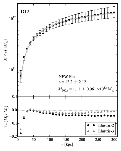
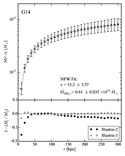
Figure 1: Top: the mass distribution $M(<r)$ derived from Illustris-1, using the D12 (left) and G14 (right) constraints on $M(<\!50\,{\rm kpc})$. Error bars represent 68% confidence intervals. The grey lines show best-fitting NFW profiles for the full mass distribution (dark matter and baryonic); the NFW fit parameters are given in the figure. The two constraints result in very different estimates of $M_{\rm 200,c}$; the concentration parameters are less disparate. Bottom: residuals between the mass distribution obtained from Illustris-1 and Illustris-2 (black circles) or Illustris-3 (grey triangles). At $r<30$ kpc, systematic differences are evident; these likely result from a combination of numerical resolution and differences in the stellar masses at fixed halo mass. Small differences of 2-5% exist at larger radii; however, such deviations are much smaller than the uncertainties we derive in Table 1.

2.2 Statistical Analysis

Our basic framework is to consider the Illustris simulation a plausible model of galaxies in our Universe, then to assign each halo in the simulation a weight based on how closely its enclosed mass at some radius (we typically use 50 kpc in what follows) matches observational data. The resulting weights for the halo sample then provide a constraint on the enclosed mass of the MW at other radii.

In more detail, we take an observational measurement of the total MW mass within a specific radius and assign a weight to each halo in the Illustris galaxy catalog: assuming the observed mass has a value of $\mu$ and an associated (Gaussian) error of $\sigma$, then the weight $W_{i}$ contributed by an individual halo $i$ with enclosed mass $M_{i}$ at the specified radius is

$$\centering W_{i}=\frac{1}{\sqrt{2\rm{\pi}}\sigma}\exp\left(\frac{-(M_{i}-\mu)^{2}}{2\sigma^{2}}\right)\,.\@add@centering$$ (1)

We can then construct the full mass or circular velocity profile and compute the total stellar or halo mass that is consistent with the observed constraint by using the distribution of weights assigned to the haloes. In this analysis, we assume that observed constraints all follow Gaussian distributions, consistent with the analyses we incorporate, but this technique can be easily extended to any other analytic or numerical probability distribution. In what follows, we quote median values and confidence intervals that are centred on the median and contain 68% of the probability distribution.

The primary observational constraint we use is the total mass of the MW within 50 kpc, $M(<\!50\,{\rm kpc})$. There are many literature estimates of the MW’s mass at approximately this scale (e.g., Wilkinson & Evans 1999; Battaglia et al. 2005; Xue et al. 2008; Brown et al. 2010; Gnedin et al. 2010; Kafle et al. 2014; Eadie et al. 2015), in large part because (1) this is approximately the distance to which large samples of blue horizontal branch (BHB) stars are currently available from surveys such as the Sloan Digital Sky Survey, and (2) the LMC lies at a Galactocentric distance of $\approx 50\,{\rm kpc}$, meaning estimates of the MW mass based on LMC’s dynamics directly constrain $M(<\!50\,{\rm kpc})$. We focus on two recent and disparate measurements of $M(<\!50\,{\rm kpc})$: Deason et al. (2012, hereafter D12), who used BHB stars and found $M(<\!50\,{\rm kpc})=4.2\pm 0.4\times 10^{11}\,M_{\odot}$, and Gibbons et al. (2014, hereafter G14), who used the Sagittarius stream to measure $M(<\!50\,{\rm kpc})=2.9\pm 0.4\times 10^{11}\,M_{\odot}$ (Gómez et al. 2015). These measurements are clearly incompatible at the $3\,\sigma$ level and therefore are useful for showing the effects of varying $M(<\!50\,{\rm kpc})$ on the inferred mass distribution at larger radii. In Sec. 3.2, we explicitly show how estimates of $M_{\rm 200,c}$ vary as a function of $M(<\!50\,{\rm kpc})$.

In principle, a complete analysis would include every dark matter halo in Illustris. In practice, however, only a relatively narrow range of masses contribute any weight to our inferences. We therefore restrict our analysis to all haloes with $M_{\rm 200,c}=(0.1-10)\times 10^{12}M_{\odot}$, which includes $14\,192$ haloes for Illustris-1, $14\,316$ haloes for Illustris-2, and $12\,885$ haloes for Illustris-3. As we show below, this mass range is more than sufficient for including all relevant haloes in our analysis and does not bias our results in any way.

3 The Mass Distribution of the MW

3.1 The MW’s radial mass profile

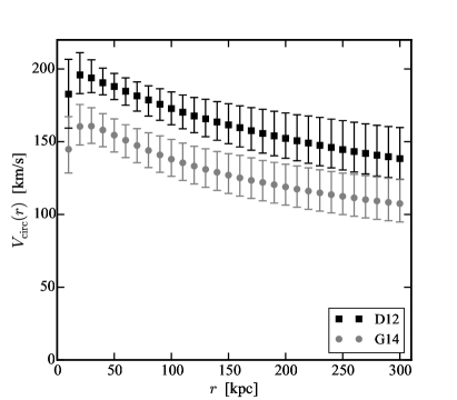
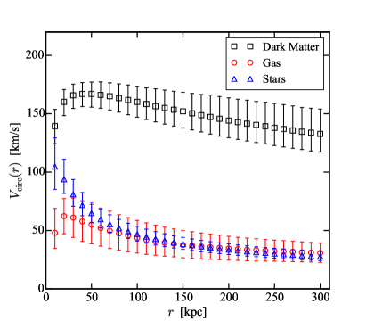
Figure 2: Circular velocity curves. Left: $V_{\rm{circ}}(r)$ for the mass profiles given in Fig. 1. The overall mass profile using G14’s constraint is lower at every Galactocentric distance compared to the profile derived using the D12 constraint, and the 68% confidence intervals are disjoint up to $280\,{\rm kpc}$. Right: a decomposition of the circular velocity profile derived using the D12 constraint (black points in the left panel of Fig. 1) into separate contributions from dark matter (black), stars (blue) and gas (red). At all radii probed here, dark matter dominates. The contribution from gas matches that from stars near a halo-centric distance of 100 kpc.

Fig. 1 presents the mass distributions obtained using the constraints on $M(<\!50\,{\rm kpc})$ from D12 (left-hand panel) and G14 (right-hand panel) from the Illustris-1 sample. The best-fitting Navarro-Frenk-White (1997, hereafter, NFW) profiles for the total mass distribution are given in the figure as well. The fits were performed over the radial range of 40–300 kpc, as we find a lack of convergence among different resolution versions of Illustris on smaller scales (see below; convergence in density profiles should occur at smaller scales, as density is a differential quantity while mass and circular velocity are cumulative quantities). Unsurprisingly, given the significantly higher value of $M(<\!50\,{\rm kpc})$ found in D12 relative to G14, the best-fitting NFW value of $M_{\rm 200,c}$ for D12 is much larger than for G14, $1.1\times 10^{12}\,M_{\odot}$ versus $0.61\times 10^{12}\,M_{\odot}$. The best fitting concentration parameters are similar: $c_{\rm 200,c}=12.2\pm 2.12$ for D12 and $c_{\rm 200,c}=13.2\pm 3.57$ for G14. Both of these concentrations are larger than those derived from large DMO simulations, which typically find $c_{\rm 200,c}\approx 8.33$ for haloes of $M_{\rm 200,c}\approx 10^{12}\,M_{\odot}$ (e.g., Dutton & Macciò 2014).

The lower panels of the figures show the fractional differences of Illustris-2 and Illustris-3 with respect to their high-resolution counterpart, with error bars representing 68% confidence intervals. There are relatively large differences between the different levels of resolution at relatively small radii ($r<30$ kpc), while differences are much less substantial farther away from Galactic Centre. With a gravitational softening length $\sim$ 1 kpc and baryonic sub-grid routines tailored specifically to the highest resolution simulation. This lack of convergence on small scales is not surprising. For instance, Schaller et al. (2016) show that the dark matter density profiles of Eagle galaxy haloes are only converged at $\approx 20$ kpc (their fig. 3). We therefore strongly caution against extrapolating the NFW fits presented in this paper to small radii ($r\la 30$ kpc). If future generations of simulations provide well-converged results at smaller radii, the dark matter fraction within $\sim 2$ disc scale lengths will likely provide important constraints on feedback models (Courteau & Dutton 2015).

The circular velocity profiles, $V_{\rm circ}(r)$, corresponding to the cumulative mass profiles of Fig. 1 are shown in the left-hand panel of Fig. 2. This highlights the large difference in the two determinations of the MW potential, as well as how this difference persists in predicted profiles out to 300 kpc. It is only at distances $>250$ kpc that the 68% confidence intervals begin to overlap.

The distribution of mass among dark matter, stars, and gas within any given radius is interesting to consider: observationally, we can measure the stellar mass with reasonable accuracy and infer the dark matter mass, but constraining the distribution of the Galaxy’s gaseous component at large distances is much more difficult (see, e.g., Gupta et al. 2012; Fang et al. 2013). In the right-hand panel of Fig. 2, we plot the circular velocity profile decomposed into the contributions from each of these components. Dark matter dominates the potential at all radii we study, and while stars substantially outweigh the gas for $r\la 50$ kpc, the two contribute approximately the same mass by $r\approx 100$ kpc.

3.2 Mass constraints within specific radii

In this subsection, we explore predictions for enclosed masses at specific radii in more detail. In particular, we are interested in understanding how observational constraints at $M(<\!50\,{\rm kpc})$ translate into inferences on masses at other radii. We consider both individual physical radii (in particular, 100 and 250 kpc) and various definitions of spherical overdensity masses ($M_{\rm 200,c}$, $M_{\rm vir}$, and $M_{\rm 200,m}$).

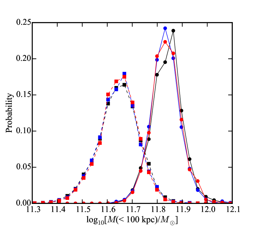
Figure 3: The probability distribution of $M(<\!100\,{\rm kpc})$ derived from the G14 (squares, connected by dashed lines) and D12 (circles, connected by solid lines) constraints on $M(<\!50\,{\rm kpc})$. The colours represent the individual resolution levels: Illustris-1 (black), Illustris-2 (blue), and Illustris-3 (red). The excellent agreement across the three levels of resolution indicates that the total mass profiles are well-converged in Illustris.

Fig. 3 presents the probability distribution for $M(<\!100\,{\rm kpc})$, with black, blue, and red symbols representing Illustris-1, Illustris-2, and Illustris-3 respectively. The results using the D12 constraint on $M(<\!50\,{\rm kpc})$ are presented as circles connected with solid lines, while those using the G14 constraint are shown as squares with dashed connecting lines. As expected, and shown previously, the D12 constraint on $M(<\!50\,{\rm kpc})$ results in a significantly higher predicted total mass within 100 kpc (approximately 0.2 dex). The smaller (relative) error quoted in D12 also results in a narrower distribution for $M(<\!100\,{\rm kpc})$.

Perhaps the most important aspect of Fig. 3 is the excellent convergence seen across the three Illustris simulations (a factor of 64 in mass resolution and 4 in force resolution). Not only is the peak or median value well converged, the entire distribution is essentially identical in each case. This indicates that, while masses on small scales (10–30 kpc) are affected by resolution and baryonic physics, enclosed masses at larger radii are not subject to such effects. The consistency of the mass distributions at large radii, subject to a constraint at 50 kpc, points to robustness of our technique for constraining the mass distribution of the MW.

Table 1: Median values, along with 68% and 90% confidence intervals, for mass measures explored in this paper; all masses are expressed in units of $10^{12}\,M_{\odot}$. In each case, we calculate values using constraints from both D12 (column 2) and G14 (column 3) on each of the three Illustris resolution levels. Good convergence across the three levels of resolution is evident.

	D12	G14
	Illustris-1
$M_{\rm 200,c}$	$1.12^{+0.370\,(0.747)}_{-0.240\,(0.357)}$	$0.612^{+0.196\,(0.384)}_{-0.148\,(0.227)}$
$M_{\rm vir}$	$1.30^{+0.511\,(1.12)}_{-0.304\,(0.445)}$	$0.711^{+0.251\,(0.522)}_{-0.179\,(0.274)}$
$M_{\rm 200,m}$	$1.48^{+0.642\,(1.49)}_{-0.361\,(0.536)}$	$0.798^{+0.306\,(0.632)}_{-0.213\,(0.319)}$
$M(<100\,{\rm kpc})$	$0.695^{+0.091\,(0.166)}_{-0.090\,(0.149)}$	$0.443^{+0.087\,(0.148)}_{-0.076\,(0.127)}$
$M(<250\,{\rm kpc})$	$1.22^{+0.334\,(0.631)}_{-0.236\,(0.355)}$	$0.736^{+0.209\,(0.406)}_{-0.164\,(0.255)}$
	Illustris-2
$M_{\rm 200,c}$	$1.06^{+0.296\,(0.674)}_{-0.196\,(0.297)}$	$0.597^{+0.166\,(0.340)}_{-0.134\,(0.206)}$
$M_{\rm vir}$	$1.24^{+0.419\,(0.954)}_{-0.243\,(0.366)}$	$0.691^{+0.213\,(0.430)}_{-0.163\,(0.250)}$
$M_{\rm 200,m}$	$1.40^{+0.490\,(1.19)}_{-0.306\,(0.442)}$	$0.766^{+0.253\,(0.543)}_{-0.186\,(0.283)}$
$M(<100\,{\rm kpc})$	$0.678^{+0.090\,(0.164)}_{-0.078\,(0.129)}$	$0.444^{+0.077\,(0.144)}_{-0.077\,(0.124)}$
$M(<250\,{\rm kpc})$	$1.17^{+0.283\,(0.588)}_{-0.194\,(0.293)}$	$0.714^{+0.184\,(0.360)}_{-0.148\,(0.229)}$
	Illustris-3
$M_{\rm 200,c}$	$1.09^{+0.332\,(0.626)}_{-0.193\,(0.304)}$	$0.614^{+0.170\,(0.332)}_{-0.135\,(0.214)}$
$M_{\rm vir}$	$1.29^{+0.441\,(0.853)}_{-0.249\,(0.386)}$	$0.712^{+0.220\,(0.434)}_{-0.160\,(0.253)}$
$M_{\rm 200,m}$	$1.46^{+0.562\,(1.252)}_{-0.293\,(0.450)}$	$0.804^{+0.256\,(0.519)}_{-0.190\,(0.298)}$
$M(<100\,{\rm kpc})$	$0.685^{+0.092\,(0.183)}_{-0.080\,(0.134)}$	$0.444^{+0.078\,(0.133)}_{-0.073\,(0.122)}$
$M(<250\,{\rm kpc})$	$1.20^{+0.300\,(0.546)}_{-0.192\,(0.302)}$	$0.741^{+0.178\,(0.342)}_{-0.148\,(0.238)}$

Inferred values of aperture masses within 100 and 250 kpc and three different spherical overdensity masses, along with 68% and 90% confidence intervals, are given in Table 1. The estimated virial mass, $M_{\rm{vir}}$, using D12 is $1.3\times 10^{12}\,M_{\odot}$, with a 90% confidence interval of $0.86-2.3\times 10^{12}\,M_{\odot}$. This is similar to the result of Boylan-Kolchin et al. (2013), who found a 90% confidence interval of $1.0-2.4\times 10^{12}\,M_{\odot}$ for $M_{\rm{vir}}$ based on the dynamics of the Leo I satellite galaxy. Using the G14 estimate of $M(<\!50\,{\rm kpc})$, we find a median value of $M_{\rm{vir}}=0.71\times 10^{12}\,M_{\odot}$ with a 90% confidence interval of $0.44-1.2\times 10^{12}\,M_{\odot}$, both of which are substantially lower than our inference based on the results of D12. These results highlight the importance of accurate determinations of $M(<\!50\,{\rm kpc})$ for understanding the large-scale properties of the MW. We note that the 99.95% confidence interval for haloes consistent with the D12 constraint is $5.17\times 10^{11}<M_{\rm 200,c}<5.06\times 10^{12}\,M_{\odot}$ (the range for the G14 constraint is $2.12\times 10^{11}<M_{\rm 200,c}<3.48\times 10^{12}\,M_{\odot}$), confirming that our range of $10^{11}\leq M_{\rm 200,c}\leq 10^{13}\,M_{\odot}$ is more than sufficient for inferences about the mass of the MW.

Figure 4: The dependence of the inferred value of $M_{\rm 200,c}$ on the input (measured) value of $M(<\!50\,{\rm kpc})$. The data points with error bars show values of $M_{\rm 200,c}$ based on our weighting procedure, assuming a 10% error in $M(<\!50\,{\rm kpc})$. The G14 and D12 determinations of $M(<\!50\,{\rm kpc})$ are highlighted with yellow and magenta vertical bands, respectively, with the widths of the bands showing the 68% confidence intervals. The best-fitting log-quadratic relation between $M(<\!50\,{\rm kpc})$ and $M_{\rm 200,c}$ (given in equation 2) is plotted as a solid grey line, while the dashed grey line shows the fit to the unweighted data; see the text for details. This relation can be used to map any constraint on $M(<\!50\,{\rm kpc})$ to an inferred value of $M_{\rm 200,c}$.

Given the uncertainties in $M(<\!50\,{\rm kpc})$, it is also important to understand how inferences of spherical overdensity masses depend on $M(<\!50\,{\rm kpc})$. To do this, we assume that $M(<\!50\,{\rm kpc})$ can be measured with an accuracy of 10% (i.e., $X\pm 0.1\,X$) and compute the resulting median value and 68% confidence intervals for $M_{\rm 200,c}$. The resulting dependence of $M_{\rm 200,c}$ on $M(<\!50\,{\rm kpc})$ is shown in Fig. 4, where the error bars show 68% confidence intervals. It is clear that there is a strong correlation between $M(<\!50\,{\rm kpc})$ and $M_{\rm 200,c}$. We fit this with a quadratic function in log space:

$$\log_{10}\left(\frac{M_{\rm 200,c}}{M_{\odot}}\right)=A+B\,\mu+C\,\mu^{2}\,,$$ (2)

$$\mu=\log_{10}\left(\frac{M(<50\,{\rm kpc})}{4\times 10^{11}\,M_{\odot}}\right)\,.$$

Fitting to the weighted results plotted in Fig. 4, we find $A=12.0,\,B=1.60,\,C=0.373$ with an rms scatter of 0.069, whereas fitting the unweighted data, we find $A=12.0,\,B=1.62,\,C=0.325$ with an rms scatter of 0.067. The latter is offset slightly higher at fixed $M(<\!50\,{\rm kpc})$, as the weighted results naturally involve averaging over the dark halo mass function within each bin, which is a steeply declining function of mass, whereas the unweighted results do not.

Equation 2 can be used to convert any constraint on $M(<\!50\,{\rm kpc})$ into a constraint on $M_{\rm 200,c}$. It is also straightforward to convert this fit to a constraint on $M_{\rm vir}$ or $M_{\rm 200,m}$, as $M_{\rm{vir}}\approx 1.17\,M_{\rm 200,c}$ and $M_{\rm 200,m}\approx 1.32\,M_{\rm 200,c}$ for the typical mass profiles in Illustris. If Equation 2 or a similar relation holds broadly for other hydrodynamic simulations with different galaxy formation physics implementations, then it will be of tremendous value for MW mass inference studies. We plan to examine this issue in more detail in future work (and see further discussion below).

3.3 The Impact of Baryonic Physics

Our primary analysis, presented over the previous subsections, makes use of the highest resolution Illustris simulation. This, and all other hydrodynamic simulations of the evolution of a representative galaxy population over cosmic time, require a number of assumptions in order to produce a realistic set of galaxies. One of the primary calibrations for Illustris, for example, was to match the $z=0$ galaxy stellar mass function. As shown in fig. 7 of Vogelsberger et al. (2014a), the galaxy formation prescriptions in Illustris result in notable changes in the total masses of dark matter haloes over a wide range in halo mass. Moreover, these changes depend on specific choices made in the galaxy formation modelling, as the galaxy formation modelling within the Eagle simulation results in substantially different effects on halo masses (see fig. 1 of Schaller et al. 2015).

It is not a priori obvious whether using the DMO run should result in similar or different predictions from the fully hydrodynamic simulation, and if the results are different, it is not clear whether they will be higher or lower. Certainly, we expect that the formation of a galaxy will lead to a more centrally concentrated mass distribution relative to the DMO run, to some extent. Adiabatic contraction of the dark matter in response to gas cooling will also tend to increase the amount of dark matter in the central regions of the halo. On the other hand, it is well established that galaxy formation must be inefficient in $\Lambda$CDM (e.g., Fukugita & Peebles 2004), meaning that only a relatively small fraction of the baryonic allotment of a dark matter halo ($\sim 20\%$ for MW-mass haloes) will be converted into stars by $z=0$. Strong feedback from galaxy formation can change the structure of dark matter haloes, reducing their mass within a given radius compared to what would be obtained in a DMO version (e.g., Vogelsberger et al. 2014b; Schaller et al. 2015). It is therefore of great interest to study precisely how inferences about the MW’s mass profile change from using DMO simulations – which, for given cosmological parameters, are uniquely predicted – to using cosmological hydrodynamic simulations.

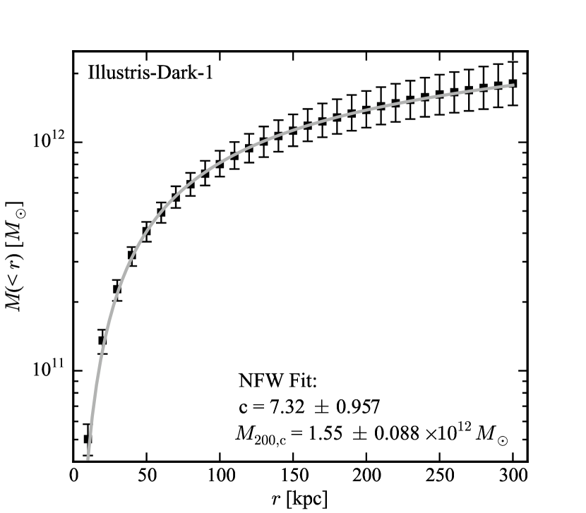
Figure 5: The cumulative mass distribution from Illustris-Dark-1 (black points with error bars), along with the best-fitting NFW profile (grey line), derived assuming the D12 constraint on $M(<\!50\,{\rm kpc})$. This figure can be directly compared to the left-hand panel of Fig. 1, which shows the same quantities from the full hydrodynamic run. While both versions of Illustris are well-fitted by NFW profiles, the fit parameters differ substantially between the two: the DMO run is fitted by a higher-mass (37% higher), lower-concentration (40% lower) halo. If DMO runs are used for modelling the MW mass distribution based on $M(<\!50\,{\rm kpc})$, or a similar constraint, this effect must be taken into account.

Table 2: Median values, along with 68% and 90% confidence intervals, for a variety of mass measures explored in this paper (similar to Table 1); all values are in units of $10^{12}\,M_{\odot}$. In contrast to Table 1, however, these results use the Illustris-Dark simulations.

	D12	G14
	Illustris-Dark-1
$M_{\rm 200,c}$	$1.57^{+0.460\,(1.28)}_{-0.343\,(0.519)}$	$0.836^{+0.296\,(0.605)}_{-0.220\,(0.336)}$
$M_{\rm vir}$	$1.88^{+0.676\,(1.65)}_{-0.445\,(0.654)}$	$0.993^{+0.382\,(0.805)}_{-0.275\,(0.417)}$
$M_{\rm 200,m}$	$2.15^{+0.841\,(1.91)}_{-0.545\,(0.808)}$	$1.12^{+0.466\,(0.997)}_{-0.318\,(0.482)}$
$M(<100\,{\rm kpc})$	$0.803^{+0.116\,(0.198)}_{-0.095\,(0.161)}$	$0.521^{+0.105\,(0.169)}_{-0.095\,(0.154)}$
$M(<250\,{\rm kpc})$	$1.62^{+0.357\,(0.830)}_{-0.299\,(0.452)}$	$0.971^{+0.283\,(0.548)}_{-0.231\,(0.355)}$
	Illustris-Dark-2
$M_{\rm 200,c}$	$1.59^{+0.515\,(1.48)}_{-0.344\,(0.531)}$	$0.838^{+0.296\,(0.593)}_{-0.219\,(0.338)}$
$M_{\rm vir}$	$1.91^{+0.712\,(1.86)}_{-0.452\,(0.681)}$	$0.991^{+0.399\,(0.793)}_{-0.268\,(0.412)}$
$M_{\rm 200,m}$	$2.18^{+0.920\,(2.19)}_{-0.565\,(0.835)}$	$1.12^{+0.476\,(1.02)}_{-0.312\,(0.478)}$
$M(<100\,{\rm kpc})$	$0.807^{+0.116\,(0.204)}_{-0.095\,(0.161)}$	$0.523^{+0.103\,(0.170)}_{-0.094\,(0.153)}$
$M(<250\,{\rm kpc})$	$1.63^{+0.396\,(0.968)}_{-0.290\,(0.462)}$	$0.971^{+0.290\,(0.548)}_{-0.221\,(0.352)}$
	Illustris-Dark-3
$M_{\rm 200,c}$	$1.61^{+0.567\,(1.39)}_{-0.349\,(0.530)}$	$0.859^{+0.302\,(0.665)}_{-0.231\,(0.348)}$
$M_{\rm vir}$	$1.96^{+0.760\,(1.98)}_{-0.488\,(0.708)}$	$1.01^{+0.389\,(0.904)}_{-0.271\,(0.423)}$
$M_{\rm 200,m}$	$2.23^{+1.00\,(2.31)}_{-0.601\,(0.868)}$	$1.15^{+0.459\,(1.09)}_{-0.316\,(0.487)}$
$M(<100\,{\rm kpc})$	$0.826^{+0.115\,(0.213)}_{-0.113\,(0.177)}$	$0.526^{+0.107\,(0.178)}_{-0.090\,(0.152)}$
$M(<250\,{\rm kpc})$	$1.65^{+0.417\,(0.901)}_{-0.311\,(0.481)}$	$0.988^{+0.292\,(0.599)}_{-0.225\,(0.361)}$

The first test we perform to gauge the effects of including galaxy formation physics on mass inferences is to rerun our analysis on the DMO versions of Illustris. Fig. 5 shows the results of applying the D12 constraint to Illustris-Dark-1. It can be directly compared to Fig. 1, in which the D12 constraint was applied to the hydrodynamic version of Illustris-1. Relative to the full Illustris simulation, inferences based on the DMO version result in a significantly higher estimate of $M_{\rm 200,c}$ ($1.5\times 10^{12}$ versus $1.1\times 10^{12}\,M_{\odot}$) and a significantly lower version of the NFW concentration ($c=7.4$ versus 12.3). Table 2 provides an alternate version of Table 1 in which all constraints are obtained using the DMO version of Illustris-1. In all cases, the net effect of using the DMO run rather than the hydrodynamic version is to infer higher values for a given aperture mass.

We can use the Illustris suite to perform an additional test of the effects of galaxy formation on the mass distribution within dark matter halos (and for accompanying inferences on the mass distribution of the MW): since Illustris and Illustris-Dark share the same initial conditions, individual dark matter halos can be matched between the two simulations (for details, see section 3.2 of Vogelsberger et al. 2014a). In this way, we can study the effects of galaxy formation on a halo-by halo basis by identifying the DMO analogue of each halo in the full Illustris run and comparing the resulting mass distributions.

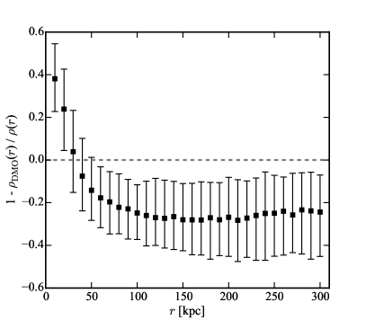
Figure 6: Fractional differences in the density (left) and enclosed mass (right) profiles between Illustris-1 and Illustris-Dark-1, where haloes are individually matched across the two simulations (see the text for details). Data points represent the median differences between Illustris-1 and Illustris-Dark-1, while error bars show the central 68% range of the data. On small scales, the inclusion of baryonic physics results in more mass at a given radius owing to the formation of the central galaxy. On large scales, however, feedback causes an overall reduction in mass on a halo-by-halo basis for the full hydrodynamic simulation relative to the DMO run. The effect in the density profile is $\sim 20\%$ at large radii, while the effect in the cumulative mass profile is $\sim 10\%$ at large distances.

Fig. 6 shows the results of this comparison, for which we use haloes in Illustris-1 falling within the 68% confidence interval of $M_{\rm 200,c}$ computed using the D12 constraint (see Table 1) – assigning equal weight to all such haloes – and their counterparts in the DMO run. The left-hand panel shows how the density profiles are affected at each radius. On small scales ($r\la 30\,{\rm kpc}$), the hydrodynamic run has higher densities on a halo-by-halo basis. This is caused by the formation of the central galaxy, both through its mass and through any adiabatic contraction. On larger scales ($r\ga 40\,{\rm kpc}$), a given halo in the hydrodynamic run is less dense than its equivalent in the DMO run by approximately 20%. This reduction in density is likely caused by outflows and the loss of gas mass (or the prevention of gas accretion). The effect on the cumulative mass distribution is shown in the right-hand panel of Fig. 6. On a halo-by-halo basis, the hydrodynamic run results in larger masses out to $\approx 100$ kpc; on larger scales, the masses in the DMO run are larger, with the difference reaching an asymptotic value of $\approx 10\%$ at 250-300 kpc. As discussed in Section 4, the details of the reduction in mass may depend on the adopted models of galaxy formation modelling.

3.4 The Stellar Mass of the Galaxy

Table 3: Inferred values of $M_{\star}$, in units of $10^{10}\,M_{\odot}$, using the D12 (column 2) and G14 (column 3) constraints on $M(<\!50\,{\rm kpc})$. The quoted errors are the 68% and 90% confidence intervals. The Illustris feedback prescriptions were calibrated for the highest-resolution simulation (Illustris-1), so perfect convergence in $M_{\star}$ across the three simulations is not expected.

	D12	G14
Illustris-1	$5.04^{+1.47\,(2.72)}_{-1.32\,(2.03)}$	$2.41^{+0.98\,(1.74)}_{-0.72\,(1.12)}$
Illustris-2	$4.09^{+1.19\,(2.15)}_{-1.15\,(1.66)}$	$1.83^{+0.76\,(1.36)}_{-0.59\,(0.90)}$
Illustris-3	$2.57^{+0.79\,(1.52)}_{-0.71\,(1.07)}$	$1.03^{+0.48\,(0.92)}_{-0.35\,(0.55)}$

We can also use the technique explored in the previous sections to compute the galaxy stellar masses from Illustris that are consistent with the adopted mass constraints at 50 kpc. Table 3 gives the median values as well as 68% and 90% confidence intervals based on the D12 and G14 constraints in each of the three Illustris resolution levels. Unlike the total enclosed mass at large radii, which is well-converged across the three different Illustris resolutions, the stellar masses in these haloes increase by a factor of $\sim 2$ from Illustris-3 to Illustris-1. This difference is not large enough to be reflected in stellar mass functions (which are reasonably similar for the different resolution levels studied here; see, e.g., Vogelsberger et al. 2013 and Torrey et al. 2014). It is larger than the uncertainty on the measured $M_{\star}$ of the MW, however: most recent estimates for the Galaxy fall in the range $M_{\star}=5-6.5\times 10^{10}\,M_{\odot}$ (e.g., McMillan 2011; Bovy & Rix 2013; Licquia & Newman 2015).

Differences in the simulated stellar masses at the factor of $\sim 2$ level are unsurprising, as the galaxy formation models used in the Illustris suite were calibrated at the resolution of Illustris-1; we would not expect the same models to work identically at significantly lower resolution. Specifically, the minimum resolution required for the feedback implementation in Illustris to produce a realistic galaxy population is not achieved in Illustris-3 (Vogelsberger et al. 2013). We therefore consider the results from Illustris-1 to be the most reasonable comparison to make with observations.

We adopt the measurement of Licquia & Newman (2015, hereafter, LN15), in which the authors used results derived in Bovy & Rix (2013) to obtain $M_{\star}=6.08\pm 1.14\times 10^{10}\,M_{\odot}$, as a representative value of the stellar mass of the MW and use it as a reference point in what follows. Comparing this number to the results for Illustris-1 in Table 3, we see that D12 agrees well with the observed value, while G14 is substantially lower. This is not surprising, given the results of Table 1. The very low value of $M_{\rm 200,c}$ obtained based on G14 is much lower than the typical value found for haloes with the stellar mass of the MW via either abundance matching (Guo et al. 2010; Behroozi et al. 2013; Moster et al. 2013), galaxy-galaxy lensing (Mandelbaum et al. 2016), or satellite kinematics (e.g., Watkins et al. 2010; Boylan-Kolchin et al. 2013). Even accounting for possible differences in halo masses of red and blue galaxies at fixed stellar mass (Mandelbaum et al. 2016), the MW would be a strong outlier if its mass is as low as the median value indicated by our analysis using the G14 constraint on $M(<\!50\,{\rm kpc})$.

As noted in Section 2, our methodology for constraining the mass profile of the MW is quite general. While we have focused on constraining the total mass at large radii based on measurements of the total mass within 50 kpc, we can instead use other quantities – for example, $M_{\star}$ – for our inference. Following the same procedure outlined in Section 2, we estimate $M(<\!50\,{\rm kpc})$, $M(<\!100\,{\rm kpc})$, and the three spherical overdensity masses used above based on LN15’s determination of $M_{\star}$; the results are presented in the second column of Table 4. The results are very similar to those obtained using the D12 determination of $M(<\!50\,{\rm kpc})$, with LN15-based estimates being 5-7% higher (the results are approximately a factor of 1.6–2 larger than G14-based estimates).

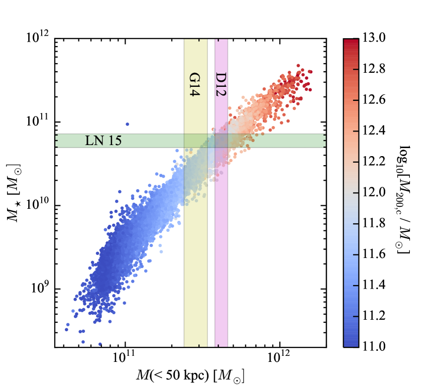
Figure 7: The correlation between $M_{\star}$ and $M(<\!50\,{\rm kpc})$ for all haloes in the Illustris-1 sample; the haloes are coloured by the value of $M_{\rm 200,c}$. Vertical shaded bands show G14 (yellow) and D12 (magenta) determinations of $M(<\!50\,{\rm kpc})$ while the horizontal band shows the LN15 determination of $M_{\star}$ for the MW. Very few haloes agree with both the G14 measurement of the total mass at 50 kpc and the MW’s stellar mass; many more of the simulated galaxies match the D12 value for $M(<\!50\,{\rm kpc})$ and the LN14 $M_{\star}$ value simultaneously.

Since $M_{\star}$ and $M(<\!50\,{\rm kpc})$ can be considered independent variables, we can also study the joint probability of obtaining various mass measures conditioned on $M_{\star}$ and $M(<\!50\,{\rm kpc})$. These joint constraints, using D12’s estimate of $M(<\!50\,{\rm kpc})$, are given in the third column of Table 4. The joint constraints are similar to both the estimates using $M_{\star}$ alone and the estimate using $M(<\!50\,{\rm kpc})$ (from D12) alone, which is a result of the good agreement of each of these estimates individually. Had we used the G14 value of $M(<\!50\,{\rm kpc})$, the constraints would have shifted substantially. This is highlighted in Fig. 7, which shows the Illustris-1 data in $M_{\star}-M(<\!50\,{\rm kpc})$ space; each halo assigned a colour according to its value of $M_{\rm 200,c}$. The intersection of the D12 and LN15 constraints falls along the main locus of the points while the G14 constraint intersects the LN 15 constraint in a part of parameter space with very few haloes. The D12 and LN15 measurements are therefore in good agreement based on the Illustris haloes, while the G14 and LN15 measurements are not.

Table 4: The 68% and 90% confidence intervals of various mass measures of the MW (all in units of $10^{12}\,M_{\odot}$) inferred using the LN15 measurement of the MW’s $M_{\star}$ alone (column 2) and jointly with the D12 constraint on $M(<\!50\,{\rm kpc})$ (column 3).

	$P(M|M_{\star})$	$P(M|M_{\star},M_{\rm D12})$
$M_{\rm 200,c}$	$1.19^{+0.62\,(1.44)}_{-0.35\,(0.52)}$	$1.13^{+0.36\,(0.80)}_{-0.22\,(0.36)}$
$M_{\rm vir}$	$1.40^{+0.81\,(1.86)}_{-0.43\,(0.64)}$	$1.33^{+0.49\,(1.20)}_{-0.29\,(0.46)}$
$M_{\rm 200,m}$	$1.60^{+1.00\,(2.15)}_{-0.53\,(0.78)}$	$1.50^{+0.65\,(1.66)}_{-0.35\,(0.54)}$
$M(<100\,{\rm kpc})$	$0.725^{+0.179\,(0.358)}_{-0.145\,(0.231)}$	$0.707^{+0.081\,(0.155)}_{-0.087\,(0.144)}$
$M(<250\,{\rm kpc})$	$1.29^{+0.51\,(1.08)}_{-0.34\,(0.51)}$	$1.23^{+0.34\,(0.67)}_{-0.21\,(0.36)}$

4 Discussion and future prospects

Figure 8: The precision attained in measurements of $M_{\rm 200,c}$ as a function of the precision in the input constraint. We consider input constraints of the total mass within 50, 80, and 100 kpc (black circles, red squares, and blue triangles, respectively) to show how more precise determinations of masses within larger radii can affect the inferred value of $M_{\rm 200,c}$. The figure shows the trade-off between precision and distance: for example, an error of 15% in $M(<\!100\,{\rm kpc})$ results in the same precision in the estimate of $M_{\rm 200,c}$ as an error of 9% in $M(<\!50\,{\rm kpc})$.

As larger samples of halo stars at greater distances become available, it may become possible to constrain the mass of the MW enclosed within 80 or even 100 kpc (see, e.g., Gnedin et al. 2010; Cohen et al. 2015 for initial work in this direction). Such measurements would have the benefit of providing stronger constraints on the virial mass of the MW. Fig. 8 shows the fractional uncertainty in $M_{\rm 200,c}$ as a function of the error in the mass contained within 50 (black circles), 80 (red squares), and 100 kpc (blue triangles). At a fixed uncertainty in $M(<r)$, the implied uncertainty in $M_{\rm 200,c}$ does indeed become smaller as one moves to greater Galactocentric distance.

The figure quantifies how improving uncertainties at a given distance will be reflected in uncertainties on $M_{\rm 200,c}$: for example, reducing the error on $M(<\!50\,{\rm kpc})$ from 10 to 5% would reduce the error on $M_{\rm 200,c}$ from 28 to 23%. On the other hand, an measurement of the mass within 80 kpc that is accurate to 10% results in an error of 22% in $M_{\rm 200,c}$, while the same accuracy on a measurement of the mass within 100 kpc of the Galaxy would yield errors of 19% in $M_{\rm 200,c}$. The figure also shows the fundamental limitations in extrapolating to $M_{\rm 200,c}$ based on measured aperture masses within smaller radii. Some level of irreducible uncertainty is unavoidable in standard cosmological models, as extrapolation from mass at a given radius to the virial radius depends on the halo concentration (e.g. Navarro et al. 1997; Bullock et al. 2001). For example, consider the recent study of Williams & Evans (2015), who found that $M(<\!50\,{\rm kpc})=4.48^{+0.15}_{-0.14}\times 10^{11}\,M_{\odot}$, or an error of approximately 3% on $M(<\!50\,{\rm kpc})$. Using this constraint, we obtain $M_{\rm 200,c}=1.25^{+0.35}_{-0.18}\times 10^{12}\,M_{\odot}$; the uncertainty on the derived value of $M_{\rm 200,c}$ remains large in spite of the high precision of the input measurement. Fig. 8 makes it clear that measurements of the mass within 50 (80, 100) kpc will result in an uncertainty on $M_{\rm 200,c}$ of no better than 23% (17%, 14%).

A central assumption of the techniques we employ here is that Illustris-1 provides a faithful representation of galaxies and the effects of galaxy formation on dark matter halo structure. Since cosmological hydrodynamic simulations are still at the point of relying on subgrid models of physics, and will be for the foreseeable future, a logical extension of our work would be to investigate predictions in future generations of simulations to test the robustness of our results. It would also be interesting to compare the results we have obtained with Illustris to the Eagle simulations, as the galaxy formation modelling employed there is somewhat different. Given the differences seen in the ratio of masses in hydrodynamic to DMO simulations in Illustris versus Eagle (compare fig. 7 of Vogelsberger et al. 2014a and fig. 1 of Schaller et al. 2015), such a comparison would be timely.

One effect that appears to be particularly important for setting the amount of mass reduction for a given halo in the hydrodynamic run relative to its counterpart in the DMO version is the underlying model of AGN feedback. Vogelsberger et al. (2014b) adopted an AGN model that drives very strong outflows, perhaps unrealistically so (Genel et al. 2014). Forthcoming updates to the Illustris suite will use modified versions of AGN feedback that are less powerful and may result in different modifications of the large-scale halo properties of galaxies, which may in turn affect how $M(<\!50\,{\rm kpc})$ maps on to $M_{\rm 200,c}$.

To explore the potential impact of this effect on our results, we use the current generation of Illustris and compare the effects of BH mass for galaxies of a fixed halo mass (we use the haloes that are closest to the median value of $M_{\rm 200,c}$ found in Illustris-Dark-1 using the D12 constraint). We rank this sample according to black hole mass and then compute the difference in mass in the hydrodynamic simulation relative to the DMO run. There is indeed a difference: the galaxies with the highest-mass black holes show a 20% reduction in their overall mass, on average, while the galaxies with the lowest mass black holes see a 10% reduction in mass compared to their DMO counterparts. The total halo mass therefore appears to depend somewhat on the choice of black hole feedback model, although this does not appear to be a large source of uncertainty in our predictions. Future generations of Illustris-like simulations with modified black hole feedback models will allow us to directly test the effects on inferences regarding the MW mass.

It is not entirely obvious how the effects of vigorous feedback propagate through our analysis, as this will depend on the change in enclosed mass within 50 kpc relative to the change in enclosed mass within larger radii. However, given that the black hole feedback in the current version of Illustris may be too effective and that the larger-mass black holes correlate with larger reductions in halo mass as compared to lower-mass black holes, it is likely that any modified prescriptions will result in slightly higher inferences on the total halo mass compared to our current results, should there be a difference.

Future work would also benefit significantly from cosmological simulations with larger volumes and higher mass resolution. Importance sampling relies on having a well-sampled parameter space, which can be an issue if not many haloes match the desired constraint(s) (see Busha et al. 2011 and González et al. 2014 for more details). Our current analysis has many haloes contributing significant weights: 870 and 2196 haloes contribute weights that are at least 10% of the maximum possible weight ($W_{\rm max}=1/\sqrt{2\rm{\pi}\sigma^{2}}$ from equation. 1) for the D12 and G14 constraints, respectively. However, if we wish to add additional restrictions – based on morphology, disc size, star formation history, or specific star formation rate, for example – the sample would likely become significantly smaller, which would be the limiting factor in the conclusions we could draw. With larger sample sizes, such concerns would be eliminated. From Fig. 7, joint constraints on $M(<\!50\,{\rm kpc})$ and $M_{\star}$ are unlikely to be strongly affected by sample size unless a much larger volume produced many haloes with much larger stellar masses at fixed halo mass [in which case, the G14 measurement of $M(<\!50\,{\rm kpc})$ would be more consistent with the simulation results than it is at present].

5 Conclusions

In this paper, we have explored how the Illustris suite can be used to inform our understanding of the mass distribution around the MW. Our main conclusions are as follows.

• The mass profiles of haloes consistent with a given constraint on $M(<\!50\,{\rm kpc})$ differ substantially between DMO and hydrodynamic versions of Illustris. Using DMO simulations to extrapolate from 50 kpc to larger radii results in an overestimate of the halo mass and an underestimate of the halo concentration.

• The effects of baryonic physics on the mass distribution of MW-like systems in Illustris are substantial: by matching haloes between the DMO and hydrodynamic simulations, we find that the latter have more mass on small scales and less mass on large scales. The asymptotic difference in the total mass density at large radii is approximately 20%.

• Since different feedback models result in very different effects on the mass distribution of dark matter even at large distances from halo centres (e.g., fig. 7 of Vogelsberger et al. 2014a compared to fig. 1 of Schaller et al. 2015), it is imperative to test how inferences on the mass of the MW depend on galaxy formation modelling.

• The mass distribution in the inner $\sim 20$ kpc is not converged in the Illustris suite [see Schaller et al. 2016 for similar results in the Eagle simulations]; this is a much larger distance than the formal convergence radius for the dark matter simulations. Results regarding the density distribution for $r\la 20$ kpc must therefore be interpreted with caution, and our best-fitting NFW profiles for the hydrodynamic simulations, which were obtained over the radial range of 40-300 kpc, should not be extrapolated to smaller radii.

• The relationship between $M(<\!50\,{\rm kpc})$ and $M_{\rm 200,c}$ in Illustris-1 is well-described by a log-quadratic relationship (equation. 2). This relationship enables the translation of any existing or future constraint on $M(<\!50\,{\rm kpc})$ into a measurement $M_{\rm 200,c}$.

• The constraints on $M(<\!50\,{\rm kpc})$ derived by D12 ($4.2\pm 0.4\times 10^{11}\,M_{\odot}$) and G14 ($2.9\pm 0.4\times 10^{11}\,M_{\odot}$) predict very different values for the virial mass of the Galaxy’s halo when using Illustris: for D12, we find $M_{\rm 200,c}=1.12^{+0.37}_{-0.24}\times 10^{12}\,M_{\odot}$ (68% confidence), while for G14, we find $M_{\rm 200,c}=0.612^{+0.196}_{-0.148}\times 10^{12}\,M_{\odot}$ (68% confidence). The values for $M_{\rm{vir}}$ and $M_{\rm 200,m}$ are 17% and 32% larger, respectively.

• Illustris haloes that have galaxies with stellar masses consistent with measurements of the MW’s $M_{\star}$ have significantly more mass within $50\,{\rm kpc}$ than the result of G14; the measurements of D12 and Williams & Evans (2015) are in much better agreement with Illustris haloes that match the observed value of $M_{\star}$. In particular, almost no haloes in Illustris jointly satisfy the G14 constraint and the LN15 measurement of $M_{\star}$ for the MW.

• From our analysis of the Illustris simulation, even an infinitely precise measurement of $M(<\!50\,{\rm kpc})$ would result in an uncertainty of $>$20% in $M_{\rm 200,c}$. The same uncertainty can be achieved for 10% errors on $M(<80\,{\rm kpc})$ or 12% errors on $M(<\!100\,{\rm kpc})$. A measurement of $M(<\!100\,{\rm kpc})$ that is accurate to 5% will translate into 15% uncertainties on $M_{\rm 200,c}$.

As ever larger and ever more realistic hydrodynamic simulations become available, so too will better statistical constraints on the mass profile of our Galaxy.

References

- Barber et al. (2014) Barber C., Starkenburg E., Navarro J. F., McConnachie A. W., Fattahi A., 2014, MNRAS, 437, 959
- Battaglia et al. (2005) Battaglia G., et al., 2005, MNRAS, 364, 433
- Behroozi et al. (2013) Behroozi P. S., Wechsler R. H., Conroy C., 2013, ApJ, 770, 57
- Besla et al. (2007) Besla G., Kallivayalil N., Hernquist L., Robertson B., Cox T. J., van der Marel R. P., Alcock C., 2007, ApJ, 668, 949
- Bovy & Rix (2013) Bovy J., Rix H.-W., 2013, ApJ, 779, 115
- Bovy et al. (2012) Bovy J., et al., 2012, ApJ, 759, 131
- Boylan-Kolchin et al. (2011a) Boylan-Kolchin M., Besla G., Hernquist L., 2011a, MNRAS, 414, 1560
- Boylan-Kolchin et al. (2011b) Boylan-Kolchin M., Bullock J. S., Kaplinghat M., 2011b, MNRAS, 415, L40
- Boylan-Kolchin et al. (2012) Boylan-Kolchin M., Bullock J. S., Kaplinghat M., 2012, MNRAS, 422, 1203
- Boylan-Kolchin et al. (2013) Boylan-Kolchin M., Bullock J. S., Sohn S. T., Besla G., van der Marel R. P., 2013, ApJ, 768, 140
- Brown et al. (2010) Brown W. R., Geller M. J., Kenyon S. J., Diaferio A., 2010, AJ, 139, 59
- Bryan & Norman (1998) Bryan G. L., Norman M. L., 1998, ApJ, 495, 80
- Bullock et al. (2001) Bullock J. S., Kolatt T. S., Sigad Y., Somerville R. S., Kravtsov A. V., Klypin A. A., Primack J. R., Dekel A., 2001, MNRAS, 321, 559
- Busha et al. (2011) Busha M. T., Wechsler R. H., Behroozi P. S., Gerke B. F., Klypin A. A., Primack J. R., 2011, ApJ, 743, 117
- Cohen et al. (2015) Cohen J. G., Sesar B., Banholzer S., PTF Consortium t., 2015, arXiv:1509.05997,
- Courteau & Dutton (2015) Courteau S., Dutton A. A., 2015, ApJ, 801, L20
- Cunningham et al. (2015) Cunningham E. C., Deason A., Guhathakurta P., Rockosi C., Kirby E., van der marel r. p., Sohn S. T., 2015, IAU General Assembly, 22, 55864
- Deason et al. (2012) Deason A. J., Belokurov V., Evans N. W., An J., 2012, MNRAS, 424, L44
- Dutton & Macciò (2014) Dutton A. A., Macciò A. V., 2014, MNRAS, 441, 3359
- Eadie et al. (2015) Eadie G. M., Harris W. E., Widrow L. M., 2015, ApJ, 806, 54
- Fang et al. (2013) Fang T., Bullock J., Boylan-Kolchin M., 2013, ApJ, 762, 20
- Fattahi et al. (2016) Fattahi A., et al., 2016, MNRAS, 457, 844
- Fukugita & Peebles (2004) Fukugita M., Peebles P. J. E., 2004, ApJ, 616, 643
- Genel et al. (2014) Genel S., et al., 2014, MNRAS, 445, 175
- Gibbons et al. (2014) Gibbons S. L. J., Belokurov V., Evans N. W., 2014, MNRAS, 445, 3788
- Gnedin et al. (2010) Gnedin O. Y., Brown W. R., Geller M. J., Kenyon S. J., 2010, ApJ, 720, L108
- Gómez et al. (2015) Gómez F. A., Besla G., Carpintero D. D., Villalobos Á., O’Shea B. W., Bell E. F., 2015, ApJ, 802, 128
- González et al. (2013) González R. E., Kravtsov A. V., Gnedin N. Y., 2013, ApJ, 770, 96
- González et al. (2014) González R. E., Kravtsov A. V., Gnedin N. Y., 2014, ApJ, 793, 91
- Guo et al. (2010) Guo Q., White S., Li C., Boylan-Kolchin M., 2010, MNRAS, 404, 1111
- Gupta et al. (2012) Gupta A., Mathur S., Krongold Y., Nicastro F., Galeazzi M., 2012, ApJ, 756, L8
- Hinshaw et al. (2013) Hinshaw G., et al., 2013, ApJS, 208, 19
- Jiang & van den Bosch (2015) Jiang F., van den Bosch F. C., 2015, MNRAS, 453, 3575
- Kafle et al. (2014) Kafle P. R., Sharma S., Lewis G. F., Bland-Hawthorn J., 2014, ApJ, 794, 59
- Kahn & Woltjer (1959) Kahn F. D., Woltjer L., 1959, ApJ, 130, 705
- Kallivayalil et al. (2006) Kallivayalil N., van der Marel R. P., Alcock C., Axelrod T., Cook K. H., Drake A. J., Geha M., 2006, ApJ, 638, 772
- Kallivayalil et al. (2013) Kallivayalil N., van der Marel R. P., Besla G., Anderson J., Alcock C., 2013, ApJ, 764, 161
- Li & White (2008) Li Y.-S., White S. D. M., 2008, MNRAS, 384, 1459
- Licquia & Newman (2015) Licquia T. C., Newman J. A., 2015, ApJ, 806, 96
- Mandelbaum et al. (2016) Mandelbaum R., Wang W., Zu Y., White S., Henriques B., More S., 2016, MNRAS, 457, 3200
- McMillan (2011) McMillan P. J., 2011, MNRAS, 414, 2446
- Moster et al. (2013) Moster B. P., Naab T., White S. D. M., 2013, MNRAS, 428, 3121
- Navarro et al. (1997) Navarro J. F., Frenk C. S., White S. D. M., 1997, ApJ, 490, 493
- Nelson et al. (2015) Nelson D., et al., 2015, arXiv:1504.00362,
- Piatek et al. (2007) Piatek S., Pryor C., Bristow P., Olszewski E. W., Harris H. C., Mateo M., Minniti D., Tinney C. G., 2007, AJ, 133, 818
- Piffl et al. (2014) Piffl T., et al., 2014, A&A, 562, A91
- Pryor et al. (2015) Pryor C., Piatek S., Olszewski E. W., 2015, AJ, 149, 42
- Rashkov et al. (2013) Rashkov V., Pillepich A., Deason A. J., Madau P., Rockosi C. M., Guedes J., Mayer L., 2013, ApJ, 773, L32
- Schaller et al. (2015) Schaller M., et al., 2015, MNRAS, 451, 1247
- Schaller et al. (2016) Schaller M., et al., 2016, MNRAS, 455, 4442
- Schaye et al. (2015) Schaye J., et al., 2015, MNRAS, 446, 521
- Schönrich (2012) Schönrich R., 2012, MNRAS, 427, 274
- Sohn et al. (2013) Sohn S. T., Besla G., van der Marel R. P., Boylan-Kolchin M., Majewski S. R., Bullock J. S., 2013, ApJ, 768, 139
- Springel et al. (2001) Springel V., White S. D. M., Tormen G., Kauffmann G., 2001, MNRAS, 328, 726
- Torrey et al. (2014) Torrey P., Vogelsberger M., Genel S., Sijacki D., Springel V., Hernquist L., 2014, MNRAS, 438, 1985
- Vera-Ciro & Helmi (2013) Vera-Ciro C., Helmi A., 2013, ApJ, 773, L4
- Vogelsberger et al. (2013) Vogelsberger M., Genel S., Sijacki D., Torrey P., Springel V., Hernquist L., 2013, MNRAS, 436, 3031
- Vogelsberger et al. (2014a) Vogelsberger M., et al., 2014a, MNRAS, 444, 1518
- Vogelsberger et al. (2014b) Vogelsberger M., et al., 2014b, Nature, 509, 177
- Wang et al. (2012) Wang J., Frenk C. S., Navarro J. F., Gao L., Sawala T., 2012, MNRAS, 424, 2715
- Wang et al. (2015) Wang W., Han J., Cooper A. P., Cole S., Frenk C., Lowing B., 2015, MNRAS, 453, 377
- Watkins et al. (2010) Watkins L. L., Evans N. W., An J. H., 2010, MNRAS, 406, 264
- Wilkinson & Evans (1999) Wilkinson M. I., Evans N. W., 1999, MNRAS, 310, 645
- Williams & Evans (2015) Williams A. A., Evans N. W., 2015, MNRAS, 454, 698
- Xue et al. (2008) Xue X. X., et al., 2008, ApJ, 684, 1143
- de Bruijne et al. (2014) de Bruijne J. H. J., Rygl K. L. J., Antoja T., 2014, in EAS Publications Series. pp 23–29 (arXiv:1502.00791), doi:10.1051/eas/1567004
- van der Marel et al. (2014) van der Marel R. P., et al., 2014, in Seigar M. S., Treuthardt P., eds, Astronomical Society of the Pacific Conference Series Vol. 480, Structure and Dynamics of Disk Galaxies. p. 43 (arXiv:1309.2014)