On the limiting Markov process of energy exchanges in a rarely interacting ball-piston gas

Abstract

We analyse the process of energy exchanges generated by the elastic collisions between a point-particle, confined to a two-dimensional cell with convex boundaries, and a ‘piston’, i.e. a line-segment, which moves back and forth along a one-dimensional interval partially intersecting the cell. This model can be considered as the elementary building block of a spatially extended high-dimensional billiard modeling heat transport in a class of hybrid materials exhibiting the kinetics of gases and spatial structure of solids. Using heuristic arguments and numerical analysis, we argue that, in a regime of rare interactions, the billiard process converges to a Markov jump process for the energy exchanges and obtain the expression of its generator.

1 Introduction

Fourier’s law of heat conduction Fourier:1822 , according to which the heat current in a material is proportional to the gradient of its local temperature, has over the last two centuries proved a powerful phenomenological tool for describing the process of energy transfer in physical systems. Yet, in spite of being well understood at a macroscopic level, the derivation of this law from a microscopic point of view arguably remains one of mathematical physics’ great challenges. Thus, in their millenium review, Bonetto et al. Bonetto:2000p13477 , after offering “a selective overview of the current state of our [then] knowledge (more precisely of our ignorance) regarding the derivation of Fourier’s Law”, proceeded to the observation that

“There is however at present no rigorous mathematical derivation of Fourier’s law […] for any system (or model) with a deterministic, e.g. Hamiltonian, microscopic evolution.”

An intriguing review of Fourier’s work and its influence with a detailed chronology of some of the main developments can be found in reference Narasimhan:1999FourierHistory . Other useful reviews devoted to the non-equilibrium statistical mechanics of low-dimensional systems include references Lepri:2003p8721 and Dhar:2008p539 .

Building upon the earlier work of Bunimovich et al. Bunimovich:1992p621 , Gaspard and Gilbert then set out in 2008 Gaspard:2008PRL101 to consider the regime of rare interactions of a class of models, henceforth referred to as GG-models, which, from the point of view of ergodic theory Bunimovich:1992p621 , are intermediate between the gas of hard balls and the periodic Lorentz gas. In general, the GG-model can be thought of as a billiard chain (or $\mathbb{Z}^{d}$-network in dimension $2\leq d\leq n$) of $n$-dimensional cells with (semi-) dispersing walls, each containing a single ball particle trapped inside it. Ball particles are moreover let to interact among neighbours under the control of the geometry of the interface between their respective cells. Hence by excluding mass transport the model focuses on energy transport solely.

A standard two-step strategy for analysing the process of heat transport is to first identify the conditions under which a mesoscopic description can be attained from the microscopic one, and second, by taking the hydrodynamic limit of the mesoscopic process to obtain, in the diffusive scaling, the heat equation at the macroscopic scale. The completion of this step also implies gaining an analytical form for the coefficient of heat conductivity.

The present work does not deal with the analysis of the second step of this strategy. In particular, we will not address the precise form of the coefficient of thermal conductivity associated with our model. We note, however, that Sasada, inspired by Stefano Olla’s remarks on the results announced in reference Gaspard:2008PRL101 , recently reported Sasada:2015 that the coefficient of heat conductivity figuring in the papers of Gaspard and Gilbert, see in particular reference Gaspard:200811P021 , corresponds to the contribution to the heat conductivity from the static correlations alone, while the true transport coefficient should also include a contribution from dynamic correlations. Whereas the latter contribution appears to be very small in comparison to the former, it does not vanish. This issue, which deserves further clarification, will be the subject of future work. Another important remark here is that for handling the second step of the strategy for GG-models the necessary spectral gap has already been obtained in reference Sasada:2015Gap ; see also reference Grigo:2012MixingRate . The analogous lower estimate of the spectral gap for the model to be introduced below is so far an open question.

We mention here that progress in this area has been paralleled by interesting prospects aiming at understanding the emergence of Fourier’s law when small noise is added to simple deterministic models, e.g. to weakly anharmonic crystals Liverani:2012Toward ; Bricmont:2007Towards , or harmonic oscillators Bernardin:2005Fourier . Such systems have also been considered in regimes of rare interactions Keller:2009p2845 ; Huveneers:2012Energy Another line of research aims at studying energy exchanges between the cells of regular lattices through the mediation of point particles Eckmann:2006Nonequilibrium ; see also reference Li:2016Local for recent progress based on the seminal work of Kipnis et al. Kipnis:1982Heat . A mixture of those two approaches was treated in reference Bonetto:2004Fourier .

Going back to the first step of the strategy described above, in the GG-model, the reduction from the deterministic dynamics at the microscopic scale to a stochastic process at the mesoscopic scale, emerges in the rare interaction limit (RIL), out of a two-stage relaxation process. In the RIL, the rate of interactions between neighbouring ball particles is arbitrarily low, which implies that a form of local equilibrium is achieved on the scale of every cell, each kept at constant energy. The convergence to local equilibrium is indeed controlled by the rate of collisions between a particle and the walls of its cell, which can be made much larger than the rate of binary collisions, i. e. of collisions between two neighbouring particles. Since averaging takes place, energy transfers between neighbouring particles behave stochastically, with every cell of the system acting as a fundamental unit whose state is specified by the energy of its ball particle. In effect, the RIL yields for the Hamiltonian kinetic equation of any finite subsystem the generator of a Markov jump process for the energies of the ball particles.

The GG-model can consist of networks of two-dimensional particles (discs) confined to identical cells Gaspard:2008NJP3004 . It can also consist of networks of three (or higher)-dimensional particles (spheres) confined to identical cells Gaspard:2012p26117 . One can think of extensions of such models with several particles trapped in every cell; their numbers may be identical or vary from cell to cell and the cells of the network may no be all identical. The dimensionality of the dynamics would then vary from cell to cell. One main goal of the present paper is to introduce yet another version of the GG-model, the simplest of its class, for which we deem the (mathematically rigorous) completion of the first step of the GG-strategy realistic.

Let us explain why we think that such a modification is necessary. The ‘simplest’ task in the original GG-programme is the treatment of a two-cell system with two interacting discs. This is actually isomorphic to a 4-dimensional semi-dispersing billiard. However, statistical properties of higher-dimensional (larger than two) billiards are so far understood exclusively for finite-horizon strictly dispersing billiards Balint:2008p1309 , and even then only under the notorious ‘complexity hypothesis’.

It was therefore suggested in reference PajorGyulai:2010p17699 that by exploiting the RIL feature of the approach of reference Gaspard:2008PRL101 , a way out of this high-dimensional quagmire would be to apply the method of ‘standard pairs’ Chernov:2009brownian , a very efficient tool stemming from the development of Markov approximation methods, which permits the use of statistical properties of lower dimensional projections of the model—in this case of well-understood planar Sinai-billiards. Be that as it may, this idea led to further technical difficulties.

For this reason we introduce below a ball-piston model, which belongs to the class of GG-models, but for which the dimension of the (simplest) isomorphic semi-dispersing billiard shrinks from 4 to 3. In this model, a disc particle caged in a two-dimensional cell with dispersing walls is let to interact with a ‘piston’ moving in a one-dimensional interval. This is isomorphic to a 3-dimensional semi-dispersing billiard. We believe that coping with its RIL is already a realistic question, which is the subject of a longer project, involving four of us, and still in progress; as to the first related publication, see balint:2015winp . Suffice it to say here that the application of the method of standard pairs to the ball-piston model is met with difficulties similar to those alluded to above. However, in this model their occurrence can be tracked and explicitly described and ultimately, as we hope, treated.

In this respect, it is worth mentioning that the method of standard pairs has already been successfully applied to models of heat conduction. Thus, in reference Dolgopyat:2011Energy a model of weakly interacting Anosov flows was considered for which the appropriate long time limit is a chain of interacting diffusion processes rather than the kind of Markov jump processes which are expected to arise in rarely interacting systems. More recently, in reference Dolgopyat:2016Encounter , the authors obtained an exponential limit law for the first encounter of two small discs on a planar Sinai billiard table, a result somewhat closer to our program.

A further aim of the present work is the calculation of several relevant characteristics of the ball-piston model, in particular:

• The unconditional and conditional mean free times of binary collisions (conditioning on the outgoing energy partition between the two particles after a binary collision);

• The transition kernel of the Markov jump process expected to emerge in the RIL;

• The restriction of the invariant measure to the binary collision surface at fixed energy.

Since some of these calculations are new, even as to their mathematical content, we endeavour to formulate our arguments in a language which we hope will be accessible to both mathematicians and physicists.

Finally, we describe a computational test of the conjecture that the emerging mesoscopic limit of the rarely interacting ball-piston model is indeed the Markov jump process we claim it is. This conjecture relies on the assumption that, in the RIL, two successive binary collisions are separated by enough wall collision events that averaging takes place. We test this by considering several outgoing laws from a binary collision and compare the ingoing laws at the next binary collision event to the relevant equilibrium law by using the Kullback-Leibler divergence Kullback:1951information . We provide numerical evidence that reducing the rate of binary collisions yields a limiting distribution of energy exchanges consistent with the expected result.

The paper is organised as follows. The ball-piston model is introduced in section 2. Section 3 is devoted to the calculation of the ball-piston mean free time and collision rate. In section 4 we introduce the notion of conditional mean free time and proceed to its calculation. The derivation of the transition kernel of the conjectured Markov jump process is provided in section 5, together with a description of our numerical test of the validity of the conjecture, as well as a discussion of numerical results. Concluding remarks are given in section 6. Specific calculations are provided in appendix A (volume integrals), appendix B (wall collision frequencies) and appendix C (restriction of the invariant measure to the binary collision surface at fixed energy).

2 Minimal ball-piston model

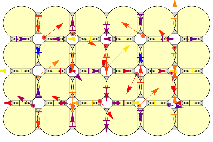
Figure 1: Ball-piston gas in a random configuration of the positions and velocities of the balls and pistons. The arrows’ lengths and colours reflect the magnitude of the corresponding particle or piston’s kinetic energy (blends of blue for low energy values, red and yellow for high energy values). Here periodic boundary conditions are applied: the piston cells of the right-most column are identical to those of the left-most column, and similarly for the upper and lower rows.

The ball-piston gas, shown in figure 1, is a collection of alternating balls and pistons, arranged in a periodic structure, with every particle confined to its own cell. Balls and pistons are particles of two different types. On the one hand, balls are point-particles with two degrees of freedom. They move in two-dimensional closed cells whose boundaries are defined by impenetrable circular obstacles placed at the vertices of a square lattice. Pistons, on the other hand, have only one degree of freedom. They are one-dimensional vertical or horizontal line-segments that are allowed to move back and forth along perpendicular intervals placed between two neighbouring ball cells. Whereas pistons are unaffected by the presence of the circular obstacles in the ball cells, they do interact elastically with balls whenever collisions occur, thereby exchanging their horizontal or vertical velocity components (both balls and pistons have unit masses). By choosing the lengths of the piston cells large enough that their extremities lay inside the ball cells (one symmetrically on each side), we allow for energy exchanges between every ball and piston pair, the likelihood of which depends on the piston’s penetration length into the ball cell. In turn, whereas mass transport of either species is prohibited by the confining walls in every cell, energy exchanges between balls and pistons induce heat transport on the scale of the ball-piston gas.

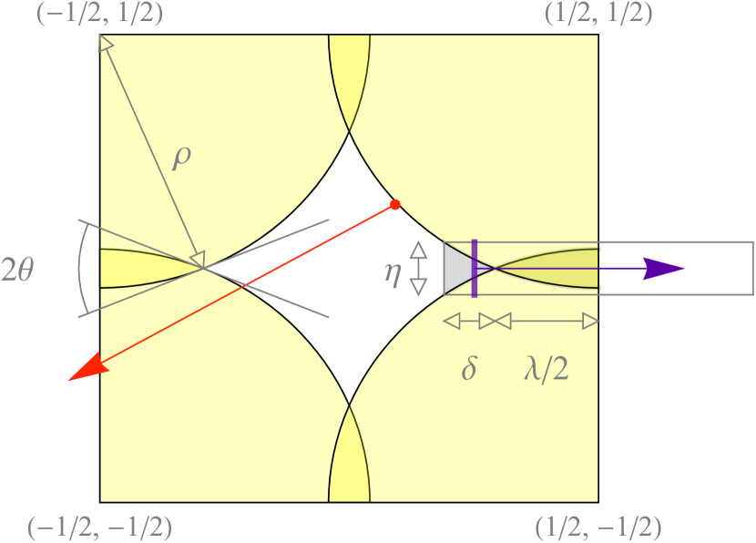
(a) Minimal ball-piston model

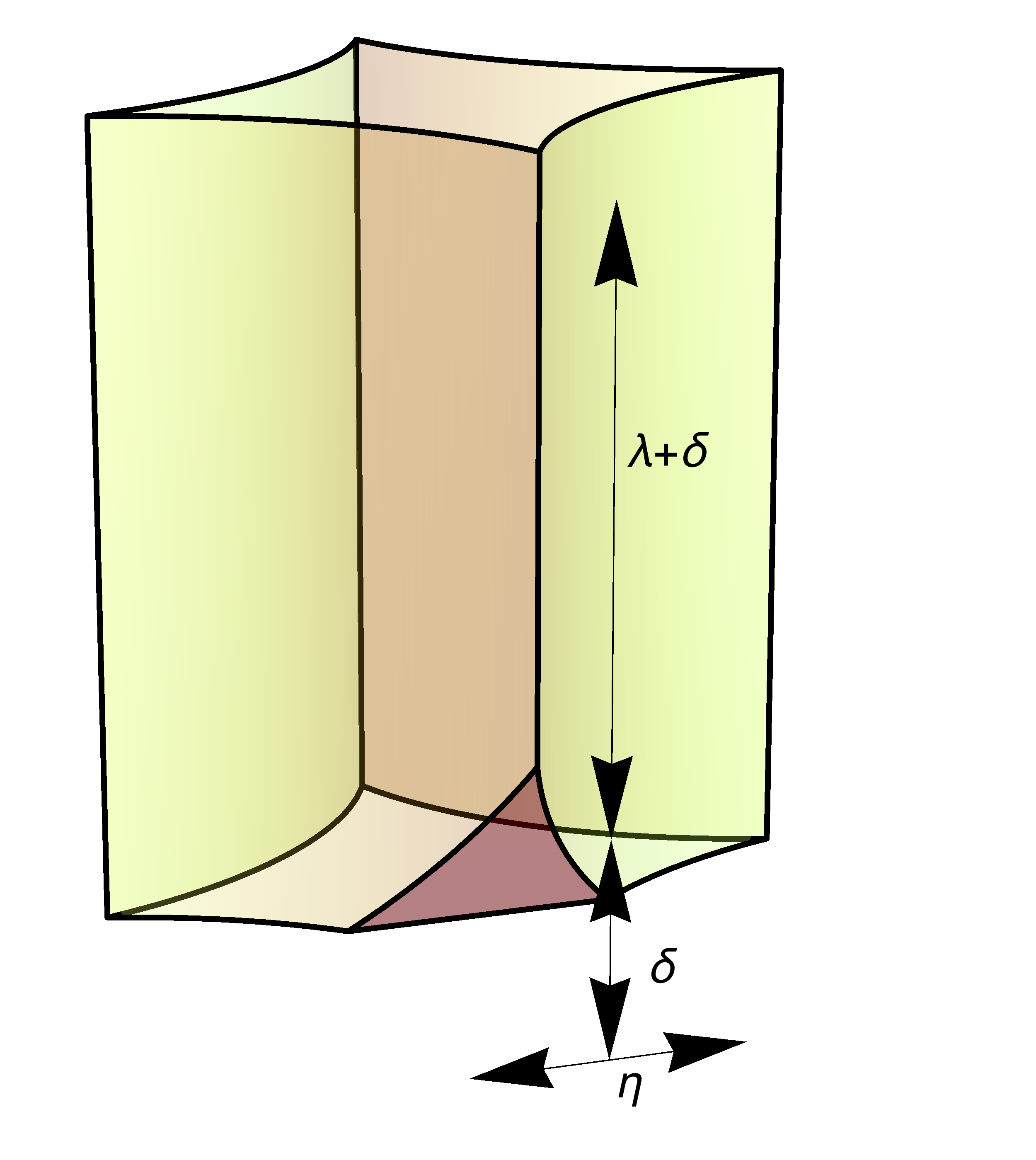
(b) Three dimensional rendition

Figure 2: (a) The minimal ball-piston model consists of a single ball-piston pair, here showed in a random configuration. The relevant parameters are defined in the text. (b) Three-dimensional rendition of the billiard boundary.

The present study focuses on a minimal version of the ball-piston gas, such as shown in figure 2(a). Here a single pair of ball and piston—in this case a horizontally moving vertical line-segment—is let to interact. This model can in fact be viewed as a three-dimensional billiard, rendered in figure 2(b): it is equivalent to the free motion of a point-particle in a three-dimensional cavity, undergoing elastic reflections upon its boundary. The corresponding collision map is a four-dimensional symplectic map.

The parameters relevant to the definition of the model are displayed in figure 2. A point-particle (ball) of unit mass moves freely in the interior of a cell (the ball cell) whose boundaries are delimited by four arc-circles of common radius $\rho$, $1/2<\rho<1/\sqrt{2}$, centered at the four corners of a unit cell, and performs elastic collisions with them. A vertical line segment of height $\eta$ and unit mass, which we call piston, moves horizontally back and forth between the two edges of an interval of length $\lambda+2\delta$ (the piston cell), centered at the middle point of the cell’s right edge, where $\lambda=\sqrt{4\rho^{2}-1}$ measures the length of the interval between the two intersections of opposite discs (and such that $\tan\theta=\lambda$). The parameter $\delta$, $0<\delta<\rho/\sqrt{2}-\lambda/2$, measures the length of penetration of the piston inside the ball cell and therefore determines the possibility of interactions between the ball and the piston. The height of the piston, $\eta=1-2\sqrt{\rho^{2}-(\lambda/2+\delta)^{2}}$, is such that, at its left-most position, it lies inside the boundary of the ball cell. The positions of the ball and piston must be initially chosen so that the ball is located to the left of the piston; the ball cannot move passed the piston.

We let $\Gamma\subset\mathbb{R}^{3}$ denote the three-dimensional ball-piston configuration space and $\partial\Gamma=\partial\Gamma_{\textsc{bp}}\cup\partial\Gamma_{\textsc{bw}}\cup\partial\Gamma_{\textsc{pw}}$ its boundary, where $\partial\Gamma_{\textsc{bp}}$ is the surface of ball-piston collisions, $\partial\Gamma_{\textsc{bw}}$ the surface of ball-wall collisions, and $\partial\Gamma_{\textsc{pw}}$ the surface of piston-wall collisions. In figure 2(b), the first term refers to the slanted darker surface of triangular shape, the second to the vertical walls, and the third to the flat top and bottom walls. The phase space of the billiard flow $\mathpzc{M}$ is the product of $\Gamma$ and $\mathbb{S}^{2}$, the sphere of unit radius in $\mathbb{R}^{3}$, $\mathpzc{M}=\Gamma\times\mathbb{S}^{2}$.

A point $\mathbf{q}=(q_{1},q_{2},q_{3})\in\Gamma$ specifies the horizontal and vertical coordinates of the ball, $(q_{1},q_{2})$, and the piston’s position, $q_{3}$. They are such that:

$$\begin{split}&(q_{1}\pm\tfrac{1}{2})^{2}+(q_{2}\pm\tfrac{1}{2})^{2}\geq\rho^{2}\,,\\ &\tfrac{1}{2}(1-\lambda)-\delta\leq q_{3}\leq\tfrac{1}{2}(1+\lambda)+\delta\,,\\ &q_{1}\leq q_{3}\,.\end{split}$$ (1)

The associated velocity vector is $\mathbf{v}=(v_{1},v_{2},v_{3})\in\mathbb{S}^{2}$. The system’s total (kinetic) energy is the sum $\epsilon_{\textsc{b}}+\epsilon_{\textsc{p}}=\tfrac{1}{2}$ of the ball and piston energies, $\epsilon_{\textsc{b}}=\tfrac{1}{2}(v_{1}^{2}+v_{2}^{2})$ and $\epsilon_{\textsc{p}}=\tfrac{1}{2}v_{3}^{2}$ respectively. The corresponding phase-space point is denoted $\mathpzc{x}=\{\mathbf{q},\mathbf{v}\}\in\mathpzc{M}$.

The phase space of the billiard map is denoted by $\mathnormal{M}$ and is given by the product of $\partial\Gamma$ and the set of vectors $\mathbf{v}\in\mathbb{S}^{2}$ whose scalar product with the unit vector normal to the billiard surface at point $\mathbf{q}\in\partial\Gamma$ is non-negative. We have the decomposition $\mathnormal{M}=\mathnormal{M}_{\textsc{bp}}\cup\mathnormal{M}_{\textsc{bw}}\cup\mathnormal{M}_{\textsc{pw}}$. We write $\mathnormal{x}=\{\mathbf{q},\mathbf{v}\}\in\mathnormal{M}$ a phase point of the billiard map.

The natural invariant measure of the flow is denoted by $\mu$ and is normalised so that $\mu(\mathpzc{M})=1$. Likewise the invariant measure of the billiard map is denoted by $\nu$ and such that $\nu(\mathnormal{M})=1$.

3 Mean free times, collision frequencies and rates

Let $S^{t}\mathpzc{x}$ denote the flow generated by the billiard dynamics on $\mathpzc{M}$. The first hitting time is the function

$$\tau_{\textsc{}}:\,\mathpzc{M}\mapsto\mathbb{R}^{+}:\,\mathpzc{x}\mapsto\inf\{t>0\,|\,S^{t}\mathpzc{x}\in\mathnormal{M}\}\,.$$ (2)

For $\mathnormal{x}\in\mathnormal{M}$, $\tau_{\textsc{}}(\mathnormal{x})$ is the return time to the billiard surface Cornfeld:book1982 , or free (flight) time Chernov:1997p1 . Similarly, we define the ball-piston free flight time to be the time separating two successive collisions between the ball and piston,

$$\tau_{\textsc{bp}}:\,\mathnormal{M}_{\textsc{bp}}\mapsto\mathbb{R}^{+}:\,\mathnormal{x}\mapsto\inf\{t>0\,|\,S^{t}\mathnormal{x}\in\mathnormal{M}_{\textsc{bp}}\}\,.$$ (3)

By ergodicity, the mean free time, which is defined to be the infinite $n$ limit of the time to the $n$th collision (with any of the surface elements of the three-dimensional billiard cavity) divided by the number of collisions $n$, almost surely exists and is independent of the initial condition if the latter is sampled with respect to the natural invariant measure of the billiard flow. It is then equal to

$$\overline{\tau}_{\textsc{}}=\mathbb{E}_{\nu}(\tau_{\textsc{}})\equiv\int_{\mathnormal{M}}\tau_{\textsc{}}(\mathnormal{x})\,\mathrm{d}\nu(\mathnormal{x})\,,$$ (4)

measured in terms of the natural invariant measure of the billiard map on $\mathnormal{M}$.

The ball-piston mean free time, i.e. the average time separating successive collisions of the ball-piston pair, is defined similarly to be

$$\overline{\tau}_{\textsc{bp}}=\mathbb{E}_{\nu_{\textsc{bp}}}(\tau_{\textsc{bp}})\equiv\int_{\mathnormal{M}_{\textsc{bp}}}\tau_{\textsc{bp}}(\mathnormal{x})\,\mathrm{d}\nu_{\textsc{bp}}(\mathnormal{x}),$$ (5)

where the measure $\nu_{\textsc{bp}}$ is $\nu$ conditioned on $\mathnormal{M}_{\textsc{bp}}$, $\nu_{\textsc{bp}}=\nu_{\textsc{}}(\mathnormal{M}_{\textsc{bp}})^{-1}\nu_{\textsc{}}|_{\mathnormal{M}_{\textsc{bp}}}$, which is the natural invariant measure of the first return map from $\mathnormal{M}_{\textsc{bp}}$ to itself.

As explained in references Chernov:1991p204 ; Chernov:1997p1 , the presence of the hitting time under the integral in equations (4) and (5) has the effect of lifting the integral on $\mathnormal{M}$ to a measure on $\mathpzc{M}$. We thus obtain an explicit formula for the ball-piston mean free time by taking the ratio between the normalising factors of the two invariant measures, that of the flow to that of the map restricted to $\mathnormal{M}_{\textsc{bp}}$. For the billiard flow, we write $\mathrm{d}\mu(\mathpzc{x})=c_{\mu}\,\mathrm{d}\mathbf{q}\,\mathrm{d}\mathbf{v}$, and, for the conditional measure of the billiard map $\mathrm{d}\nu_{\textsc{bp}}(\mathnormal{x})=c_{\nu_{\textsc{bp}}}\mathrm{d}\mathbf{q}\,\mathrm{d}\mathbf{v}\,(\mathbf{v}\cdot\mathbf{n})$, where $\mathbf{n}$ is the ($\mathbf{q}$-independent) unit vector normal to $\partial\Gamma_{\textsc{bp}}$,

$$\mathbf{n}=\frac{1}{\sqrt{2}}(-1,0,1)\,.$$ (6)

These normalising factors are, respectively,

$$c_{\mu}^{-1} =\int_{\Gamma}\mathrm{d}\mathbf{q}\,\int_{\mathbb{S}^{2}}\mathrm{d}\mathbf{v}\,=4\pi|\Gamma|\,,$$ (7)

$$c_{\nu_{\textsc{bp}}}^{-1} =\int_{\partial\Gamma_{\textsc{bp}}}\mathrm{d}\mathbf{q}\,\int_{\mathbb{S}^{2}:\,\mathbf{v}\cdot\mathbf{n}>0}\mathrm{d}\mathbf{v}\,(\mathbf{v}\cdot\mathbf{n})=\pi|\partial\Gamma_{\textsc{bp}}|\,,$$ (8)

where we have substituted $|\mathbb{S}^{2}|=4\pi$ and $|\mathbb{B}^{2}|=\pi$, the volume of the unit ball in $\mathbb{R}^{2}$.

The ratio between equations (7) and (8) yields the ball-piston mean free time, or mean return time to the ball-piston collision surface,

$$\overline{\tau}_{\textsc{bp}}=\frac{c_{\nu_{\textsc{bp}}}}{c_{\mu}}=\frac{4|\Gamma|}{|\partial\Gamma_{\textsc{bp}}|}\,.$$ (9)

This formula is but a special case of the well-known formula for the mean-free time of three-dimensional billiards Chernov:1997p1 .

The simple geometry of the minimal ball-piston model allows for an explicit computation of the volume and surface integrals in equation (9):

$$|\Gamma| =(\lambda+2\delta)\Big{\{}1-\lambda-\rho^{2}\big{[}\pi-4\arctan(\lambda)\big{]}\Big{\}}$$ (10)

$$\quad-\frac{1}{24}\Big{\{}2\delta(\lambda+4\delta)+\big{[}1-\sqrt{1-4\delta(\lambda+\delta)}\big{]}\big{[}2+4\delta(\lambda+\delta)+3\lambda^{2}\big{]}\Big{\}}$$ (11)

$$\quad-\frac{1}{2}\rho^{2}(\lambda+2\delta)\Big{[}\arctan\lambda-\arctan\frac{\lambda+2\delta}{\sqrt{1-4\delta(\lambda+\delta)}}\Big{]}\,,$$ (12)

$$|\partial\Gamma_{\textsc{bp}}| =\frac{1}{2\sqrt{2}}\Big{\{}(\lambda+2\delta)\big{[}2-\sqrt{1-4\delta(\delta+\lambda)}\big{]}-\lambda\Big{\}}$$ (13)

$$\quad+\sqrt{2}\rho^{2}\Big{[}\arctan\lambda-\arctan\frac{\lambda+2\delta}{\sqrt{1-4\delta(\delta+\lambda)}}\Big{]}\,;$$ (14)

see appendix A for details.

The small $\delta$ regime, when ball-piston collisions become arbitrarily rare, is of particular interest, as discussed in section 5. On the one hand, $\lim_{\delta\to 0}|\Gamma|$ is simply the area (A.1) multiplied by $\lambda$, the length of the piston’s interval of motion (1) in the limit $\delta\to 0$. On the other hand, the piston’s height in this regime is $\eta\simeq 2\lambda\delta$, so that the region the piston can penetrate inside the ball cell forms approximately a triangle of area $\lambda\delta^{2}$ in the $(q_{1},q_{2})$ plane. As discussed in appendix A, this triangle is essentially the projection on the ball cell of the Poincaré section of ball-piston collisions. Accordingly, $|\partial\Gamma_{\textsc{bp}}|\simeq\sqrt{2}\lambda\delta^{2}$. To leading order, the inverse of the mean free time is therefore proportional to the parameter squared,

$$\lim_{\delta\to 0}(\overline{\tau}_{\textsc{bp}}\delta^{2})^{-1}=\frac{1}{2\sqrt{2}}\Big{[}1-\lambda-\rho^{2}\big{(}\pi-4\arctan\lambda\big{)}\Big{]}^{-1}\,,$$ (15)

which, up to the prefactor, is the inverse of area (A.1).

Since the number of collisions up to some time $t$ almost surely increases like $t/\overline{\tau}_{\textsc{}}$ as $t\to\infty$, it is natural to call $\overline{f}_{\textsc{}}\equiv\overline{\tau}_{\textsc{}}^{-1}$ the collision frequency. However, $\overline{f}_{\textsc{}}$ can also be identified with a probability rate. Indeed, ergodicity implies that $\overline{f}_{\textsc{}}$ is also, for any time interval, the expected number of collisions measured in that time interval divided by its length. Thus, in particular, $\overline{f}_{\textsc{}}$ can be expressed using the probability to observe at least one collision up to time $t$, which is $\mu\big{(}\{\mathpzc{x}\in\mathpzc{M}\,|\,S^{t}\mathpzc{x}\cap\mathnormal{M}\neq\emptyset\}\big{)}$. Namely,

$$\overline{f}_{\textsc{}}=\lim_{t\to 0}\frac{1}{t}\mu\big{(}\{\mathpzc{x}\in\mathpzc{M}\,|\,S^{t}\mathpzc{x}\cap\mathnormal{M}\neq\emptyset\}\big{)}\,.$$ (16)

By the same token, $\overline{f}_{\textsc{bp}}\equiv\overline{\tau}_{\textsc{bp}}^{-1}$ is the ball-piston collision frequency, and also defines a probability rate in the sense that

$$\overline{f}_{\textsc{bp}}=\lim_{t\to 0}\frac{1}{t}\mu\big{(}\{\mathpzc{x}\in\mathpzc{M}\,|\,S^{t}\mathpzc{x}\cap\mathnormal{M}_{\textsc{bp}}\neq\emptyset\}\big{)}\,.$$ (17)

We emphasise that equations (16) and (17) justify referring to $\overline{f}_{\textsc{}}$ and $\overline{f}_{\textsc{bp}}$ as collision (probability) rates, regardless of the actual distributions of the waiting times $\tau_{\textsc{}}$ and $\tau_{\textsc{bp}}$. In particular, these quantities may have distributions which are not exponential, and, accordingly, the collision event process may not be Poisson.

Similar considerations apply to the ball-wall and piston-wall collision events. We refer to appendix B for a computation of the corresponding return times.

4 Conditional mean free times, collision frequencies and rates

Say the billiard flow is in a stationary regime and we are observing the successive collision events that result in energy exchanges between the ball and piston. Let us assume we are only interested in a marginal set of events such that the ball-piston energy partition has the value $\{\epsilon_{\textsc{b}},\epsilon_{\textsc{p}}\}$, with $\epsilon_{\textsc{b}}+\epsilon_{\textsc{p}}=\tfrac{1}{2}$. Specifically, we ask: for points $\mathnormal{x}\in\mathnormal{M}$ whose velocity vectors $\mathbf{v}=(v_{1},v_{2},v_{3})$ are such that $\tfrac{1}{2}(v_{1}^{2}+v_{2}^{2})=\epsilon_{\textsc{b}}$ and $\tfrac{1}{2}v_{3}^{2}=\epsilon_{\textsc{p}}$, what is the corresponding mean free time? A formula similar to equation (5) is obtained for this quantity, which we call the conditional mean free time:

$$\overline{\tau}_{\textsc{bp}}(\epsilon_{\textsc{p}})=\mathbb{E}_{\nu_{\textsc{bp}|\epsilon_{\textsc{p}}}}(\tau_{\textsc{bp}})\equiv\int_{\mathnormal{M}_{\textsc{bp}}(\epsilon_{\textsc{p}})}\tau_{\textsc{bp}}(x)\,\mathrm{d}\nu_{\textsc{bp}|\epsilon_{\textsc{p}}}(x)\,.$$ (18)

where the measure $\nu_{\textsc{bp}|\epsilon_{\textsc{p}}}$ is the measure $\nu_{\textsc{bp}}$ conditioned on the subset $\mathnormal{M}_{\textsc{bp}}(\epsilon_{\textsc{p}})\subset\mathnormal{M}_{\textsc{bp}}$ of phase-space points $\mathnormal{x}=\{\mathbf{q},\mathbf{v}\}$ such that $\mathbf{q}\in\partial\Gamma_{\textsc{bp}}$ and $\mathbf{v}=(v_{1},v_{2},v_{3})\in\mathbb{S}^{2}$ with $v_{3}=\pm\sqrt{2\epsilon_{\textsc{p}}}$ and $v_{3}>v_{1}$ (consistent with $\mathbf{v}\cdot\mathbf{n}>0$).

To obtain an explicit formula, it is enough to transpose the normalising factors in equations (7) and (8) to the associated subvolumes of phase-space,

$$\overline{\tau}_{\textsc{bp}}(\epsilon_{\textsc{p}})=\frac{c_{\nu_{\textsc{bp}|\epsilon_{\textsc{p}}}}}{c_{\mu_{\epsilon_{\textsc{p}}}}}\,.$$ (19)

These normalising factors are computed as follows. Note that the three-dimensional velocity vector $\mathbf{v}$ is allowed to take values on two circles of radii $\sqrt{1-2\epsilon_{\textsc{p}}}$ parallel to the plane $(v_{1},v_{2})$, whose two heights correspond to the two allowed signs of the piston velocity $v_{3}$,

$$\begin{split}v_{1}&=\sqrt{1-2\epsilon_{\textsc{p}}}\cos\alpha\,,\\ v_{2}&=\sqrt{1-2\epsilon_{\textsc{p}}}\sin\alpha\,,\\ v_{3}&=\sigma\sqrt{2\epsilon_{\textsc{p}}}\,,\end{split}$$ (20)

where $\sigma=\pm 1$; see figure 6 in appendix C. The inverse of the factor $c_{\mu_{\epsilon_{\textsc{p}}}}$ is thus the product of the volume $|\Gamma|$ and twice the perimeter of the unit circle,

$$c_{\mu_{\epsilon_{\textsc{p}}}}^{-1}=\int_{\Gamma}\mathrm{d}\mathbf{q}\,\int_{2\times\mathbb{S}^{1}}\mathrm{d}\mathbf{v}\,=4\pi|\Gamma|\,,$$ (21)

which turns out to be identical to $c_{\mu}$, equation (7). This quantity must indeed be independent of the parameter $\epsilon_{\textsc{p}}$, since only the orientations of the velocities are relevant. This is, however, not so of the factor $c_{\nu_{\textsc{bp}|\epsilon_{\textsc{p}}}}$, which, as described in appendix C, is found to be:

$$c_{\nu_{\textsc{bp}|\epsilon_{\textsc{p}}}}^{-1} =\int_{\partial\Gamma_{\textsc{bp}}}\mathrm{d}\mathbf{q}\,\int_{2\times\mathbb{S}^{1}:\,\mathbf{v}\cdot\mathbf{n}>0}\mathrm{d}\mathbf{v}\,(\mathbf{v}\cdot\mathbf{n})\,,$$ (22)

$$=4\pi|\partial\Gamma_{\textsc{bp}}|\begin{cases}\tfrac{1}{\pi}\left[\sqrt{\tfrac{1}{2}-2\epsilon_{\textsc{p}}}+\sqrt{\epsilon_{\textsc{p}}}\arcsin\sqrt{\frac{\displaystyle\epsilon_{\textsc{p}}}{\displaystyle\tfrac{1}{2}-\epsilon_{\textsc{p}}}}\right]\,,&\epsilon_{\textsc{p}}<\tfrac{1}{4}\,,\\ \tfrac{1}{2}\sqrt{\epsilon_{\textsc{p}}}\,,&\epsilon_{\textsc{p}}\geq\tfrac{1}{4}\,.\end{cases}$$ (23)

To perform an actual measurement of the conditional mean free time (19), one must sample initial conditions with respect to the density

$$c_{\nu_{\textsc{bp}|\epsilon_{\textsc{p}}}}(\mathbf{v}\cdot\mathbf{n})_{+}$$ (24)

on $\mathnormal{M}_{\textsc{bp}}$, where $(x)_{+}=x$ if $x>0$, and $0$ otherwise; see appendix C for details. It is, however, worth noting the conditional mean free time (19) may be computed most simply as follows. Consider an equilibrium time series of the billiard dynamics and select the subset of ball-piston collision events with energy partitions close to the desired one. Indeed, definition (18) can immediately be extended to arbitrary energy intervals. Considering, in particular, the interval $(\epsilon_{\textsc{p}}-\tfrac{1}{2}\varepsilon,\epsilon_{\textsc{p}}+\tfrac{1}{2}\varepsilon)$ for small $\varepsilon>0$, we have the identity

$$\overline{\tau}_{\textsc{bp}}(\epsilon_{\textsc{p}})=\lim_{\varepsilon\to 0}\frac{\overline{\tau}_{\textsc{bp}}(\epsilon_{\textsc{p}}-\tfrac{1}{2}\varepsilon,\epsilon_{\textsc{p}}+\tfrac{1}{2}\varepsilon)}{\varepsilon}\,,$$ (25)

which guarantees the convergence, as one decreases the parameter $\varepsilon$, to the desired result of a measurement performed on a coarser set.

The reason that makes the conditional mean free time (19) particularly interesting is that its inverse $\overline{f}_{\textsc{bp}}(\epsilon_{\textsc{p}})\equiv\overline{\tau}_{\textsc{bp}}(\epsilon_{\textsc{p}})^{-1}$ can again be viewed as a rate,

$$\overline{f}_{\textsc{bp}}(\epsilon_{\textsc{p}})=\lim_{t\to 0}\frac{1}{t}\mu_{\epsilon_{\textsc{p}}}\big{(}\{\mathpzc{x}\in\mathpzc{M}\,|\,S^{t}\mathpzc{x}\cap\mathnormal{M}_{\textsc{bp}}\neq\emptyset\}\big{)}\,.$$ (26)

In the rare interaction limit $\delta\to 0$, we expect the conditional distribution of $\tau_{\textsc{bp}}(\epsilon_{\textsc{p}})$ to indeed become exponential, with rate $\overline{f}_{\textsc{bp}}(\epsilon_{\textsc{p}})$, consistent with the expectation that the energy process converges to a Markov jump process; see section 5.

Note that, by definition of $c_{\nu_{\textsc{bp}|\epsilon_{\textsc{p}}}}$, we recover the inverse of $c_{\nu_{\textsc{bp}}}$ after integrating the inverse of the former quantity over the values of the piston energy $\epsilon_{\textsc{p}}$, weighted by the density of its marginal equilibrium distribution, a Beta distribution of shape parameters $\tfrac{1}{2}$ and $1$. This relation implies a similar one between the ball-piston conditional collision rate (26) and the collision rate (17),

$$\int_{0}^{\tfrac{1}{2}}\mathrm{d}\epsilon_{\textsc{p}}\,\frac{1}{\sqrt{2\epsilon_{\textsc{p}}}}\overline{f}_{\textsc{bp}}(\epsilon_{\textsc{p}})=\overline{f}_{\textsc{bp}}\,.$$ (27)

This does not contradict the identities $\overline{f}_{\textsc{bp}}(\epsilon_{\textsc{p}})=\overline{\tau}_{\textsc{bp}}(\epsilon_{\textsc{p}})^{-1}$ and $\overline{f}_{\textsc{bp}}=\overline{\tau}_{\textsc{bp}}^{-1}$.

The product of the mean free time (9) by the collision rate (26) allows to define a dimensionless energy-dependent collision frequency which is independent of the billiard geometry,

$$\phi_{\textsc{bp}}(\epsilon_{\textsc{p}})\equiv\overline{\tau}_{\textsc{bp}}\overline{f}_{\textsc{bp}}(\epsilon_{\textsc{p}})=\begin{cases}\frac{4}{\pi}\left[\sqrt{\tfrac{1}{2}-2\epsilon_{\textsc{p}}}+\sqrt{\epsilon_{\textsc{p}}}\arcsin\sqrt{\frac{\displaystyle\epsilon_{\textsc{p}}}{\displaystyle\tfrac{1}{2}-\epsilon_{\textsc{p}}}}\right]\,,&0<\epsilon_{\textsc{p}}\leq\tfrac{1}{4}\,,\\ 2\sqrt{\epsilon_{\textsc{p}}}\,,&\tfrac{1}{4}<\epsilon_{\textsc{p}}\leq\tfrac{1}{2}\,.\end{cases}$$ (28)

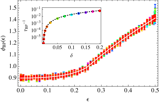
Figure 3: Numerical computations of the product of the mean free time by the conditional collision rate, compared with the rescaled ball-piston collision frequency, $\phi_{\textsc{bp}}(\epsilon_{\textsc{p}})$, given by equation (28) (solid white curve), plotted as function of the piston energy $\epsilon_{\textsc{p}}=\epsilon$ (with the ball energy $\epsilon_{\textsc{b}}=\tfrac{1}{2}-\epsilon$). The parameter $\delta$ takes on a number of different values which can be read off the horizontal axis of the graph in the inset. There we show the numerical computations of the inverse of the mean free time as function of $\delta$ in comparison to equation (9) (dotted black curve). The colours of the data in the inset match those of the data sets in the main graph.

A numerical computation of the conditional mean free times of the minimal ball-piston model for a range of energy values was carried out taking $\rho=(\sqrt{3}3-2)/(5\sqrt{2})\simeq 0.5296$ and varying $\delta$ in the interval $0<\delta\leq 0.2$. The comparison with equation (28) is shown in figure 3. All data sets collapse on the analytic result, within an accuracy that is controlled by the number of initial conditions. For each parameter $\delta$ and energy value $\epsilon_{\textsc{p}}$, a number of $10^{4}$ initial conditions were generated with respect to the distribution of density (24). A comparison between equation (9) and numerical computations of the mean free time is shown in the inset of the same figure.

5 Stochastic reduction and limiting Markov process

The mean free time (9) determines the time scale of the stochastic process of energy exchanges of the ball-piston pair. Given an equilibrium ingoing energy configuration $\{\epsilon_{\textsc{b}},\epsilon_{\textsc{p}}\}$, at collision, the density of the equilibrium measure (24) yields the probability to find the system in the outgoing energy configuration $\{\widetilde{\epsilon_{\textsc{b}}},\widetilde{\epsilon_{\textsc{p}}}\}$.

5.1 Stochastic kernel

Prior to resolving the collision event, let us assume the system is in the configuration $(\mathbf{q},\mathbf{v})$, with position vector $\mathbf{q}\in\partial\Gamma_{\textsc{bp}}$ and velocity vector $\mathbf{v}$ such that the ball-piston pair has the energy configuration $\{\epsilon_{\textsc{b}},\epsilon_{\textsc{p}}\}$, parametrised by equation (20), and such that $\mathbf{v}\cdot\mathbf{n}<0$. After the collision, we must have the outgoing velocity vector $\mathbf{\tilde{v}}$, $\mathbf{\tilde{v}}\cdot\mathbf{n}>0$, with components

$$\begin{split}\widetilde{v_{1}}&=\sqrt{2\widetilde{\epsilon_{\textsc{b}}}}\cos\tilde{\alpha}=\sigma\sqrt{2\epsilon_{\textsc{p}}}\,,\\ \widetilde{v_{2}}&=\sqrt{2\widetilde{\epsilon_{\textsc{b}}}}\sin\tilde{\alpha}=\sqrt{2\epsilon_{\textsc{b}}}\sin\alpha\,,\\ \widetilde{v_{3}}&=\tilde{\sigma}\sqrt{2\widetilde{\epsilon_{\textsc{p}}}}=\sqrt{2\epsilon_{\textsc{b}}}\cos\alpha\,.\end{split}$$ (29)

In particular, $\widetilde{\epsilon_{\textsc{b}}}=\epsilon_{\textsc{p}}+\epsilon_{\textsc{b}}\sin^{2}\alpha$ and $\widetilde{\epsilon_{\textsc{p}}}=\epsilon_{\textsc{b}}\cos^{2}\alpha$.

The probability per unit time of this transition is

$$\frac{|\partial\Gamma_{\textsc{bp}}|}{4\pi|\Gamma|}(\sqrt{\epsilon_{\textsc{b}}}\cos\alpha-\sigma\sqrt{\epsilon_{\textsc{p}}})_{+}\mathrm{d}\alpha\,,$$ (30)

which we now wish to rewrite in terms of the outgoing piston energy $\widetilde{\epsilon_{\textsc{p}}}$. From the third line in equation (29), we see that $\alpha$ can be written explicitly in terms of the ingoing and outgoing energies,

$$\sqrt{\epsilon_{\textsc{b}}}\cos\alpha=\tilde{\sigma}\sqrt{\widetilde{\epsilon_{\textsc{p}}}}\,.$$ (31)

The measure element thus transforms to

$$\mathrm{d}\alpha=\mathrm{d}\widetilde{\epsilon_{\textsc{p}}}\frac{1}{2\sqrt{\widetilde{\epsilon_{\textsc{p}}}(\epsilon_{\textsc{b}}-\widetilde{\epsilon_{\textsc{p}}})}}\,\Theta_{\textsc{h}}\!(\epsilon_{\textsc{b}}-\widetilde{\epsilon_{\textsc{p}}})\,,$$ (32)

where we have inserted the Heaviside step function, $\,\Theta_{\textsc{h}}\!(x)=1$ if $x\geq 0$, $0$ otherwise, to keep track of the condition $\mathbf{v}\cdot\mathbf{n}<0$.

Now summing over $\sigma$ and $\tilde{\sigma}$ and multiplying the above expression by 2, which reflects the fact that the collision process is independent of the sign of $v_{2}$, the probability per unit time (30) transposes to

$$W(\epsilon_{\textsc{b}},\epsilon_{\textsc{p}}|\widetilde{\epsilon_{\textsc{b}}},\widetilde{\epsilon_{\textsc{p}}})\,\mathrm{d}\widetilde{\epsilon_{\textsc{p}}}\,,$$ (33)

where the probability density,

$$W(\epsilon_{\textsc{b}},\epsilon_{\textsc{p}}|\widetilde{\epsilon_{\textsc{b}}},\widetilde{\epsilon_{\textsc{p}}}) =\frac{|\partial\Gamma_{\textsc{bp}}|}{4\pi|\Gamma|}\sum_{\sigma,\tilde{\sigma}}\frac{(\tilde{\sigma}\sqrt{\widetilde{\epsilon_{\textsc{p}}}}-\sigma\sqrt{\epsilon_{\textsc{p}}})_{+}}{\sqrt{\widetilde{\epsilon_{\textsc{p}}}(\epsilon_{\textsc{b}}-\widetilde{\epsilon_{\textsc{p}}})}}\,\Theta_{\textsc{h}}\!(\epsilon_{\textsc{b}}-\widetilde{\epsilon_{\textsc{p}}})\,,$$ (34)

$$=\frac{|\partial\Gamma_{\textsc{bp}}|}{2\pi|\Gamma|}\frac{\mathrm{max}(\sqrt{\widetilde{\epsilon_{\textsc{p}}}},\sqrt{\epsilon_{\textsc{p}}})}{\sqrt{\widetilde{\epsilon_{\textsc{p}}}(\epsilon_{\textsc{b}}-\widetilde{\epsilon_{\textsc{p}}})}}\,\Theta_{\textsc{h}}\!(\epsilon_{\textsc{b}}-\widetilde{\epsilon_{\textsc{p}}})\,,$$ (35)

can be interpreted as the rate of probability of a transfer of energy $\zeta=\epsilon_{\textsc{b}}-\widetilde{\epsilon_{\textsc{b}}}$ from the ball at energy $\epsilon_{\textsc{b}}$ to the piston whose energy changes from $\epsilon_{\textsc{p}}$ to $\widetilde{\epsilon_{\textsc{p}}}=\epsilon_{\textsc{p}}+\zeta$, $-\epsilon_{\textsc{p}}\leq\zeta\leq\epsilon_{\textsc{b}}$.

By construction, we recover the conditional collision rate (26) after integrating equation (35) over $\zeta$,

$$\overline{f}_{\textsc{bp}}(\epsilon_{\textsc{p}})=\int\mathrm{d}\zeta\,W(\epsilon_{\textsc{b}},\epsilon_{\textsc{p}}|\epsilon_{\textsc{b}}-\zeta,\epsilon_{\textsc{p}}+\zeta)\,.$$ (36)

5.2 Convergence to a Markov process

Although equation (35) is a property of the equilibrium system, we argue that it also provides an accurate description of the energy exchange process between the ball and piston away from equilibrium, provided we consider the limiting regime of rare interactions—that is, when the penetration length of the piston into the domain of the ball is arbitrarily small, $\delta\ll 1$. Indeed, under this assumption, the ball and piston typically undergo many wall-collision events between every binary collision, so that a relaxation to equilibrium of the ball-piston pair at fixed energies effectively takes place before the next occurrence of a binary collision.

As a result, in the limiting regime of rare interactions, the process of energy exchanges is expected to converge to a Markov jump process with kernel (35). Indeed, the Markov property essentially means that if one knows not only the present energy partition, but also has information about its history, this additional information does not improve one’s ability to predict the future evolution of the energy partition. Correspondingly, convergence to a Markov process means that if $\delta>0$ decreases, then information about the past influences the future less and less. So we need to see that if we start the system with a given energy partition between the disk and piston, but away from the equilibrium measure (conditioned on the energy surface), then, as $\delta\to 0$, we measure nearly the same jump rates as in (35). This is expected to hold exactly because of the relaxation to (conditional) equilibrium during the many wall-collisions that typically precede the first energy exchange.

According to this argument, the time-evolution of the ball-piston pair energy distribution $P(\{\epsilon_{\textsc{b}},\epsilon_{\textsc{p}}\},t)$ may be described by the following master equation:

$$\partial_{t}P(\{\epsilon_{\textsc{b}},\epsilon_{\textsc{p}}\},t) =\int\mathrm{d}\zeta\,\Big{[}W(\epsilon_{\textsc{b}}+\zeta,\epsilon_{\textsc{p}}-\zeta|\epsilon_{\textsc{b}},\epsilon_{\textsc{p}})P(\{\epsilon_{\textsc{b}}+\zeta,\epsilon_{\textsc{p}}-\zeta\},t)$$ (37)

$$\qquad-W(\epsilon_{\textsc{b}},\epsilon_{\textsc{p}}|\epsilon_{\textsc{b}}-\zeta,\epsilon_{\textsc{p}}+\zeta)P(\{\epsilon_{\textsc{b}},\epsilon_{\textsc{p}}\},t)\Big{]}\,.$$ (38)

The method used to derive this result relies on geometric and measure-theoretic arguments. An alternative approach based on kinetic theory, such as used in references Gaspard:2008NJP3004 ; Gaspard:200811P021 ; Gaspard:2009P08020 , yields the same results.

5.3 Numerical test of the Markov property

We want to further substantiate the assertion that—with an appropriate rescaling of time—the actual process of energy exchanges produced by the ball-piston billiard has a well-defined limit when $\delta\to 0$, and that the limiting process is indeed Markovian and described by equation (37). Based on the heuristic arguments presented in section 5.2, we should therefore check that, as $\delta$ decreases, the collision rate and post-collision energy distribution become arbitrarily close to the limits associated with the process generated by equation (37), independently of our information about the past, that is, independently of the (non-equilibrium) initial distribution we sample our energy partition with.

Moreover the notion that we have limited information about the past reflects a lack of precise knowledge of the initial conditions. Our initial distribution should therefore be smooth. Finally, since there is, of course, no hope of checking that this is convergence holds for every initial distribution, we pick a specific family of smooth initial measures on the energy surface, and check convergence for it.

In particular we consider, for different values of $\delta$, an initial state $(\mathbf{q},\mathbf{v})$ of the billiard map, with position $\mathbf{q}$ uniformly distributed on the collision surface $\partial\Gamma_{\textsc{bp}}$ and velocity $\mathbf{v}$ as in (20), such that $\mathbf{v}\cdot\mathbf{n}>0$, with angle $\alpha$ and sign $\sigma$ now distributed away from the distribution of density (24), and measure the distribution of ingoing velocities at the first ball-piston collision event. The velocity $\mathbf{v}$, now such that $\mathbf{v}\cdot\mathbf{n}<0$, may again be parametrised as in (20), with values of $\alpha$ and $\sigma$ different from the outgoing initial velocity, but $\epsilon_{\textsc{p}}$ unchanged. Since we are considering a marginal velocity distribution, apart from the two values of the sign $\sigma$, this distribution is a function of a single real variable, $\alpha$. Irrespective of the choice of piston energy $\epsilon_{\textsc{p}}$ (with ball energy $\epsilon_{\textsc{b}}=\tfrac{1}{2}-\epsilon_{\textsc{p}}$), we expect to find a distribution of ingoing $\alpha$ and $\sigma$ that, as $\delta\to 0$, becomes arbitrarily close to the distribution on the constant $\epsilon_{\textsc{p}}$ circles induced by the equilibrium measure.

That is because, in the absence of ball-piston collisions, the wall-collision events will typically induce a relaxation of the billiard dynamics to the measure of density (24), which is a true invariant measure of the non-interacting ball-piston dynamics when their energies are fixed to the corresponding values. In other words, when $\delta$ is small, the billiard dynamics is likely to perform many wall collision events before first hitting the ball-piston collision surface $\mathnormal{M}_{\textsc{bp}}$. The first hitting distribution is thus expected to converge to the distribution of density (24), which happens to be an equilibrium distribution of the ball-piston dynamics when interactions are turned off ($\delta\equiv 0$).

To be specific, let

$$h_{\epsilon_{\textsc{p}}}^{(n)}(\alpha,\sigma)\propto(\sqrt{\epsilon_{\textsc{b}}}\cos\alpha-\sigma\sqrt{\epsilon_{\textsc{p}}})_{+}^{n}\,,$$ (39)

and normalise these densities so that $\sum_{\sigma=\pm 1}\int\mathrm{d}\alpha\,h_{\epsilon_{\textsc{p}}}^{(n)}(\alpha,\sigma)=1$. In particular, the density $h_{\epsilon_{\textsc{p}}}^{(0)}$ is uniform on the set $\mathbf{v}\cdot\mathbf{n}>0$ and $h_{\epsilon_{\textsc{p}}}^{(1)}$ is the density (24) induced by the equilibrium distribution, albeit with a different normalisation.

(a) $\epsilon=0.03125$, $\delta=0.325$

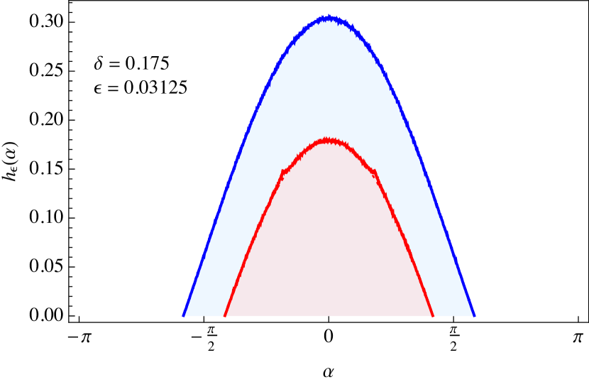
(b) $\epsilon=0.03125$, $\delta=0.175$

(c) $\epsilon=0.03125$, $\delta=0.0125$

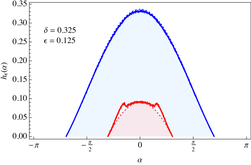
(d) $\epsilon=0.125$, $\delta=0.325$

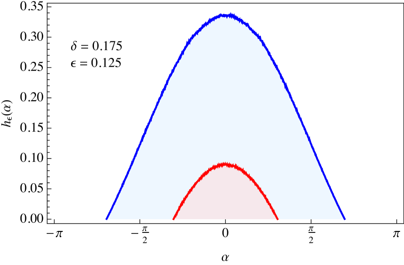
(e) $\epsilon=0.125$, $\delta=0.175$

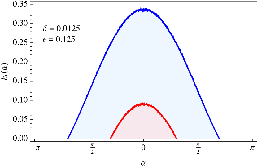
(f) $\epsilon=0.125$, $\delta=0.0125$

(g) $\epsilon=0.25$, $\delta=0.325$

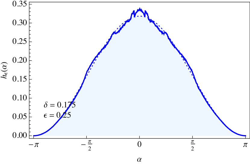
(h) $\epsilon=0.25$, $\delta=0.175$

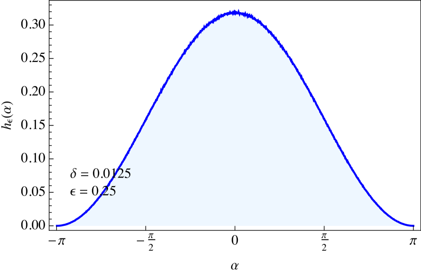
(i) $\epsilon=0.25$, $\delta=0.0125$

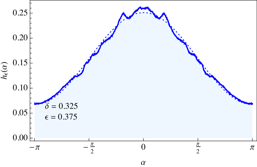
(j) $\epsilon=0.375$, $\delta=0.325$

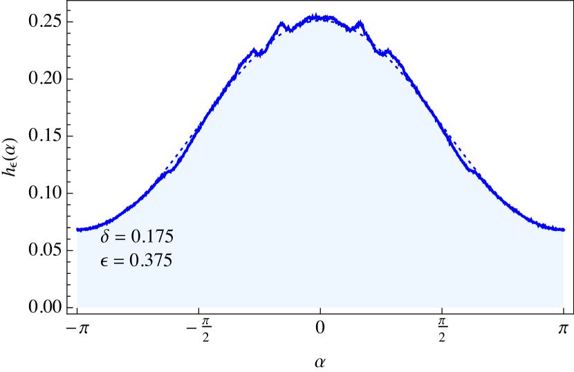
(k) $\epsilon=0.375$, $\delta=0.175$

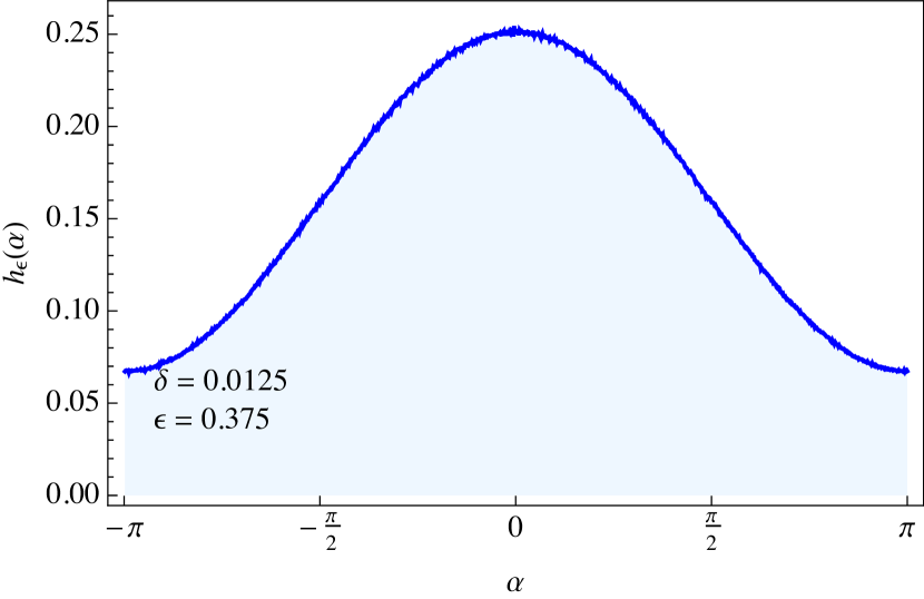
(l) $\epsilon=0.375$, $\delta=0.0125$

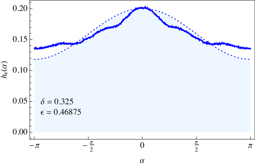
(m) $\epsilon=0.469$, $\delta=0.325$

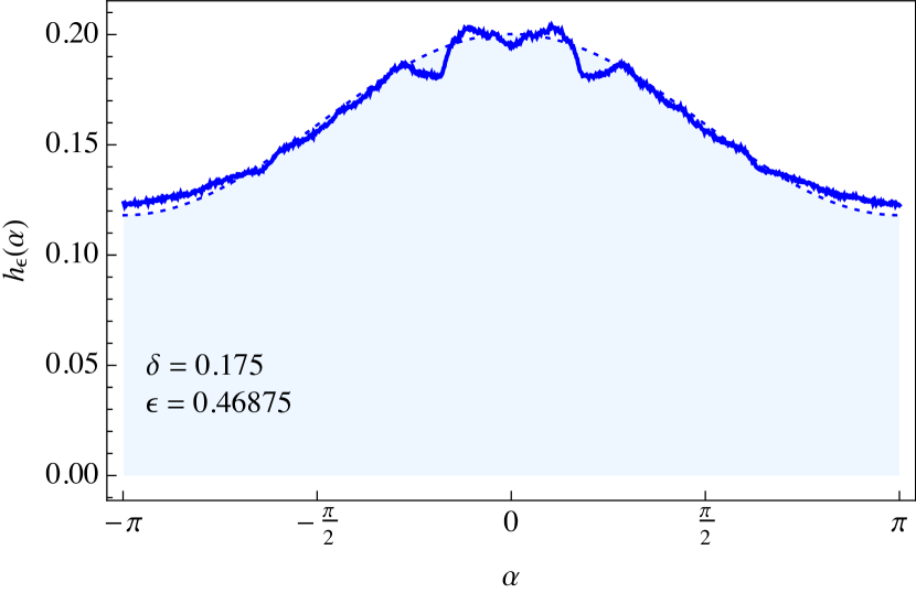
(n) $\epsilon=0.469$, $\delta=0.175$

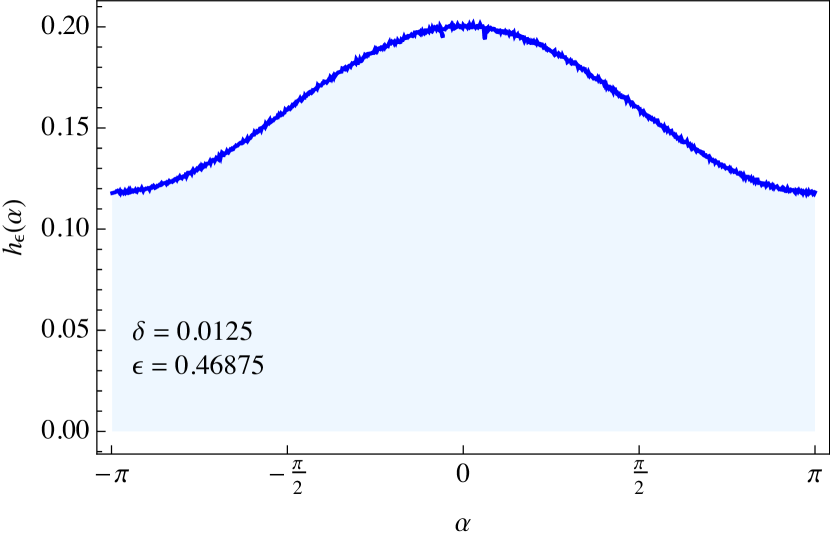
(o) $\epsilon=0.469$, $\delta=0.0125$

Figure 4: Histograms of the measured ingoing first hit velocity distributions obtained from outgoing distributions (39) with exponent $n=0$. The horizontal axes show the angle values $\alpha$. The parts of the densities corresponding to $\sigma=+1$ are shown in solid blue lines and to $\sigma=-1$ in solid red lines (only for $\epsilon_{\textsc{p}}<1/4$). Every curve is compared to the corresponding density induced by the equilibrium measure (filled areas). Each row in the figure corresponds to a fixed value of $\epsilon_{\textsc{p}}$ and each column to a fixed value of $\delta$, decreasing from left to right.

In figure 4, we plot the histograms of the ingoing velocity distributions obtained by sampling initial conditions with respect to the non-equilibrium density $h_{\epsilon_{\textsc{p}}}^{(0)}$. Each subfigure corresponds to a different value of $\delta$, varied horizontally, and $\epsilon_{\textsc{p}}$, varied vertically. Histograms are measured by dividing the intervals of allowed values of $\alpha$ into $10^{3}$ bins. As seen from the figure, the differences between the measured distributions and the corresponding distributions induced by the equilibrium measure are never large, but are most noticeable when $\delta$ is large. To quantify the convergence of the measured distributions to those induced by the equilibrium measure, we computed the (coarse grained) relative entropy of the measured distribution with respect to $h_{\epsilon_{\textsc{p}}}^{(1)}$, also known as Kullback-Leibler divergence Kullback:1951information . Using the notation $\tilde{h}_{\epsilon_{\textsc{p}}}^{(n)}$ to denote the ingoing distribution into which the initial distribution $h_{\epsilon_{\textsc{p}}}^{(n)}$ evolves until the first energy exchange,

$$D_{\textsc{kl}}(\tilde{h}_{\epsilon_{\textsc{p}}}^{(n)}|h_{\epsilon_{\textsc{p}}}^{(1)})=\sum_{\sigma=\pm 1}\int\mathrm{d}\alpha\,\tilde{h}_{\epsilon_{\textsc{p}}}^{(n)}(\alpha,\sigma)\log\frac{\tilde{h}_{\epsilon_{\textsc{p}}}^{(n)}(\alpha,\sigma)}{h_{\epsilon_{\textsc{p}}}^{(1)}(\alpha,\sigma)}\,,$$ (40)

where the integral over $\alpha$ is evaluated by summing the measured averaged density over the total number of bins. The results of measurements of this quantity using different outgoing velocity distributions $h_{\epsilon_{\textsc{p}}}^{(n)}$, $n=0,1,5,10$, and exact values for the density $h_{\epsilon_{\textsc{p}}}^{(1)}(\alpha,\sigma)$ in the denominator of equation (40) are shown in figure 5. Whereas the decay to the equilibrium noise level of the Kullback-Leibler divergence with the parameter $\delta$ appears to be qualitatively different when the piston energies are larger than the ball energies or vice versa, our measurements clearly show a systematic return to the statistics induced by the equilibrium measure as the parameter $\delta\to 0$ and thus provide a confirmation of the observations drawn from figure 4.

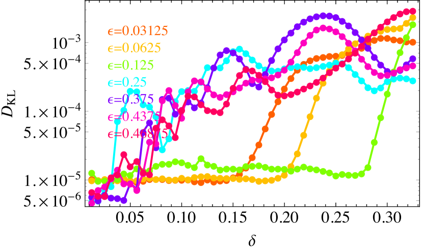
(a) $n=0$

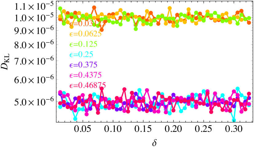
(b) $n=1$

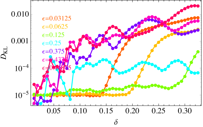
(c) $n=5$

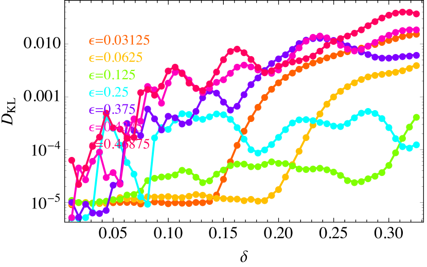
(d) $n=10$

Figure 5: The Kullback-Leibler divergence (40) of the measured density of the ingoing velocity distributions relative to the equilibrium density (24) provides a quantitative measurement of the convergence of the former to the latter as the parameter $\delta\to 0$. Data obtained by sampling initial conditions with respect to the densities $h_{\epsilon_{\textsc{p}}}^{(n)}$, (a) $n=0$, (b) $n=1$, (c) $n=5$, (d) $n=10$ are displayed as functions of the penetration length $\delta$ of the piston into the ball cell. The oscillatory behaviour observed for some values of the energies appears to be logarithmic with respect to $\delta$. In panel (b), we compare the numerically obtained values of the equilibrium distribution $h_{\epsilon_{\textsc{p}}}^{(1)}$ to its analytic expression (24), and thus obtain a useful benchmark to gauge the accuracy within which equilibrium statistics can be reached. The factor $2$ between the sets with $\epsilon_{\textsc{p}}<1/4$ and $\epsilon_{\textsc{p}}\geq 1/4$ is due to the fact that the phase space is divided into twice as many cells when $\epsilon_{\textsc{p}}<1/4$ compared to $\epsilon_{\textsc{p}}\geq 1/4$.

5.4 Moments of the kernel

We end this section by noting that the stochastic evolution (37) proves particularly useful to study energy exchanges in rarely interacting systems consisting of many particles, such as the ball-piston gas shown in figure 1. In this context, we note that the first three moments of the energy transfer rate share the symmetries observed in other models Gaspard:2009P08020 .

Thus, given the canonical ball-piston energy distribution, which is the product of Gamma distributions of shape parameters respectively $\tfrac{1}{2}$ and $1$, and common scale parameter (the temperature) $\beta^{-1}$,

$$P^{(\textsc{can})}_{\beta}(\epsilon_{\textsc{b}},\epsilon_{\textsc{p}})=\frac{\beta^{3/2}}{\sqrt{\pi\epsilon_{\textsc{p}}}}\exp[-\beta(\epsilon_{\textsc{b}}+\epsilon_{\textsc{p}})]\,,$$ (41)

the zeroth moment of the energy transfer rate, similar to $\overline{f}_{\textsc{bp}}(\epsilon_{\textsc{p}})$, equation (36), but without the assumption $\epsilon_{\textsc{b}}=\tfrac{1}{2}-\epsilon_{\textsc{p}}$,

$$f(\epsilon_{\textsc{b}},\epsilon_{\textsc{p}}) \equiv\int\mathrm{d}\zeta\,W(\epsilon_{\textsc{b}},\epsilon_{\textsc{p}}|\epsilon_{\textsc{b}}-\zeta,\epsilon_{\textsc{p}}+\zeta)\,,$$ (42)

$$=\frac{|\partial\Gamma_{\textsc{bp}}|}{|\Gamma|}\begin{cases}\frac{1}{\pi}\left[\sqrt{\epsilon_{\textsc{b}}-\epsilon_{\textsc{p}}}+\sqrt{\epsilon_{\textsc{p}}}\arcsin\sqrt{\frac{\displaystyle\epsilon_{\textsc{p}}}{\displaystyle\epsilon_{\textsc{b}}}}\right]\,,&\epsilon_{\textsc{b}}>\epsilon_{\textsc{p}}\,,\\ \tfrac{1}{2}\sqrt{\epsilon_{\textsc{p}}}\,,&\epsilon_{\textsc{b}}\leq\epsilon_{\textsc{p}}\,,\end{cases}$$

the first moment,

$$j(\epsilon_{\textsc{b}},\epsilon_{\textsc{p}}) \equiv\int\mathrm{d}\zeta\,\zeta\,W(\epsilon_{\textsc{b}},\epsilon_{\textsc{p}}|\epsilon_{\textsc{b}}-\zeta,\epsilon_{\textsc{p}}+\zeta)\,,$$ (43)

$$=\frac{|\partial\Gamma_{\textsc{bp}}|}{|\Gamma|}\begin{cases}\frac{1}{6\pi}\Big{[}(4\epsilon_{\textsc{b}}-7\epsilon_{\textsc{p}})\sqrt{\epsilon_{\textsc{b}}-\epsilon_{\textsc{p}}}\\ \quad+3(\epsilon_{\textsc{b}}-2\epsilon_{\textsc{p}})\sqrt{\epsilon_{\textsc{p}}}\arcsin\sqrt{\epsilon_{\textsc{p}}/\epsilon_{\textsc{b}}}\Big{]}\,,&\epsilon_{\textsc{b}}>\epsilon_{\textsc{p}}\,,\\ \frac{1}{4}(\epsilon_{\textsc{b}}-2\epsilon_{\textsc{p}})\sqrt{\epsilon_{\textsc{p}}}\,,&\epsilon_{\textsc{b}}\leq\epsilon_{\textsc{p}}\,,\end{cases}$$

and the second moment,

$$h(\epsilon_{\textsc{b}},\epsilon_{\textsc{p}}) \equiv\int\mathrm{d}\zeta\,\zeta^{2}W(\epsilon_{\textsc{b}},\epsilon_{\textsc{p}}|\epsilon_{\textsc{b}}-\zeta,\epsilon_{\textsc{p}}+\zeta)\,,$$ (44)

$$=\frac{|\partial\Gamma_{\textsc{bp}}|}{|\Gamma|}\begin{cases}\frac{1}{15\pi}\Big{\{}8(\epsilon_{\textsc{b}}-\epsilon_{\textsc{p}})^{5/2}+15\Big{[}-\frac{3}{8}\epsilon_{\textsc{p}}(\epsilon_{\textsc{b}}-2\epsilon_{\textsc{p}})\sqrt{\epsilon_{\textsc{b}}-\epsilon_{\textsc{p}}}\\ \quad+\sqrt{\epsilon_{\textsc{p}}}(\frac{3}{8}\epsilon_{\textsc{b}}^{2}-\epsilon_{\textsc{b}}\epsilon_{\textsc{p}}+\epsilon_{\textsc{p}}^{2})\arcsin\sqrt{\epsilon_{\textsc{p}}/\epsilon_{\textsc{b}}}\Big{]}\Big{\}}\,,&\epsilon_{\textsc{b}}>\epsilon_{\textsc{p}}\,,\\ \tfrac{1}{2}\sqrt{\epsilon_{\textsc{p}}}(\frac{3}{8}\epsilon_{\textsc{b}}^{2}-\epsilon_{\textsc{b}}\epsilon_{\textsc{p}}+\epsilon_{\textsc{p}}^{2})\,,&\epsilon_{\textsc{b}}\leq\epsilon_{\textsc{p}}\,,\end{cases}$$

all satisfy the following identities, involving averages with respect to the canonical measure (41):

$$\langle f(\epsilon_{\textsc{b}},\epsilon_{\textsc{p}})\rangle^{(\textsc{can})}_{\beta}=\frac{\beta^{2}}{2}\langle(\epsilon_{\textsc{b}}-\epsilon_{\textsc{p}})j(\epsilon_{\textsc{b}},\epsilon_{\textsc{p}})\rangle^{(\textsc{can})}_{\beta}=\frac{\beta^{2}}{2}\langle h(\epsilon_{\textsc{b}},\epsilon_{\textsc{p}})\rangle^{(\textsc{can})}_{\beta}=\frac{1}{\sqrt{2\pi\beta}}\frac{|\partial\Gamma_{\textsc{bp}}|}{|\Gamma|}\,.$$ (45)

In the limit $\delta\to 0$ of rare interactions, this is

$$\lim_{\delta\to 0}\delta^{-2}\langle f(\epsilon_{\textsc{b}},\epsilon_{\textsc{p}})\rangle^{(\textsc{can})}_{\beta}=\frac{1}{\sqrt{\pi\beta}}\Big{[}1-\lambda-\rho^{2}\big{(}\pi-4\arctan\lambda\big{)}\Big{]}^{-1}\,,$$ (46)

which provides an approximation of the heat conductivity of the ball-piston gas. This will be the subject of a separate publication.

6 Conclusions

In reference Gaspard:2008PRL101 a family of billiard models was introduced in the hope of proving suitable for deriving the heat equation. It is moreover believed it will be possible to determine the actual expression of the associated coefficient of heat conductivity. Such an achievement would bring to completion a programme aiming at explaining macroscopic laws from deterministic microscopic assumptions, one of mathematical physics great outstanding challenges.

These models, which combine the kinetics of gases of hard balls with the periodic structure of crystalline solids, lend themselves to a systematic analysis, whose tools were made available in no small part thanks to the pioneering works of David Ruelle and Yasha Sinai. The authors of Gaspard:2008PRL101 outlined a simple two-step strategy to attain their goal: (i) going from the microscopic scale to a mesoscopic one (micro-to-meso), and (ii) from that scale to the macroscopic one (meso-to-macro). Moreover, they also realised their programme on the level of analytic calculations with precise physical meaning.

Among realistic models to study Fourier’s law, billiard models are generally most amenable to a rigorous derivation of both mesoscopic and macroscopic laws from deterministic microscopic assumptions, however delicate their technical analysis. It has therefore been a top priority of the community to provide a mathematically sound proof completing the approach outlined above. Our main goal here has been to suggest a new addition to the family of Gaspard-Gilbert models, for which a mathematical treatment of the micro-to-meso step is a distinctly realistic task.

In this paper, we focused on the description of the ball-piston model and the computation of several quantities characterising its statistical properties. The limit of rare ball-piston interactions provides a meaningful interpretation, both physically and mathematically, of some of these properties at the level of a mesoscopic description. Namely, energy exchanges are described by a Markov jump process with a precise form of the transition kernel. The complete mathematical discussion is postponed to subsequent publications (as to the first of these, see balint:2015winp ).

We have, in addition, devised a statistical procedure, making use of the Kullback-Leibler divergence, to test quantitatively whether the limit of rare interactions of the minimal ball-piston model indeed possesses the Markov property. Our numerical results are affirmative and help shed new light on the approach to this limit. Our procedure can be put to use in other models of the GG family and its application will be described elsewhere.

Appendix A Collision volume

To determine the volume $|\Gamma|$ of configuration space, note that when $q_{3}>(1-\lambda)/2$, the volume of all possible positions $q_{1}$ and $q_{2}$ is

$$4\int_{0}^{(1-\lambda)/2}\mathrm{d}\,q\left[\tfrac{1}{2}-\sqrt{\rho^{2}-\left(q-\tfrac{1}{2}\right)^{2}}\right]=1-\lambda-\rho^{2}\big{(}\pi-4\arctan\lambda\big{)}\,.$$ (A.1)

When $q_{3}<(1-\lambda)/2$, we must subtract from the above area the quantity

$$2 \int_{q_{3}}^{(1-\lambda)/2}\mathrm{d}\,q\left[\tfrac{1}{2}-\sqrt{\rho^{2}-\left(q-\tfrac{1}{2}\right)^{2}}\right]=\frac{1}{2}-\frac{\lambda}{4}-q_{3}-\frac{1-2q_{3}}{4}\sqrt{4\rho^{2}-(1-2q_{3})^{2}}$$ (A.2)

$$\quad+\rho^{2}\left[\arctan\lambda-\arctan\frac{1-2q_{3}}{\sqrt{4\rho^{2}-(1-2q_{3})^{2}}}\right]\,.$$ (A.3)

We therefore obtain the total volume of configuration space (12) by multiplying equation (A.1) by $\lambda+2\delta$ and subtracting the integral of equation (A.3) over $q_{3}$ from $(1-\lambda)/2-\delta$ to $(1-\lambda)/2$.

To compute the collision surface integral, note that the position coordinates on $\partial\Gamma_{\textsc{bp}}$ are bounded according to

$$\begin{split}&\tfrac{1}{2}(1-\lambda)-\delta\leq q_{1}=q_{3}\leq\tfrac{1}{2}(1-\lambda)\,,\\ &-\tfrac{1}{2}+\sqrt{\rho^{2}-(q_{1}-\tfrac{1}{2})^{2}}\leq q_{2}\leq\tfrac{1}{2}-\sqrt{\rho^{2}-(q_{1}-\tfrac{1}{2})^{2}}\end{split}$$ (A.4)

Its projection on the $(q_{1},q_{2})$ plane is the area (A.3) evaluated at $q_{3}=(1-\lambda)/2-\delta$. Since the surface itself makes an angle $\pi/4$ with respect to the $(q_{1},q_{2})$ plane, we obtain for $|\partial\Gamma_{\textsc{bp}}|$ the expression given by equation (14).

Appendix B Ball-wall and piston-wall return times

Wall collision return times of the piston and ball can be computed in ways similar to equation (9),

$$\begin{split}\overline{\tau}_{\textsc{pw}}&=\frac{4|\Gamma|}{|\partial\Gamma_{\textsc{pw}}|}\,,\\ \overline{\tau}_{\textsc{bw}}&=\frac{4|\Gamma|}{|\partial\Gamma_{\textsc{bw}}|}\,,\end{split}$$ (B.1)

where $|\partial\Gamma_{\textsc{pw}}|$ and $|\partial\Gamma_{\textsc{bw}}|$ are the areas of piston-wall and ball-wall collisions. The former corresponds to the area of all positions $q_{1}$ and $q_{2}$ such that $q_{3}=(1\pm\lambda)/2\pm\delta$, which is parallel to the $(q_{1},q_{2})$ plane and twice the area (A.1) minus the projection of the collision surface $|\partial\Gamma_{\textsc{bp}}|$ (14) on this plane, and the latter to the positions $q_{1},q_{2}$ such that $(q_{1}\pm\tfrac{1}{2})^{2}+(q_{2}\pm\tfrac{1}{2})^{2}=\rho^{2}$ while $q_{1}<q_{3}$, with $q_{3}$ integrated over the interval (1). That is,

$$|\partial\Gamma_{\textsc{pw}}| =2\Big{[}1-\lambda-\rho^{2}\big{(}\pi-4\arctan\lambda\big{)}\Big{]}-\frac{1}{\sqrt{2}}|\partial\Gamma_{\textsc{bp}}|\,,$$ (B.2)

and

$$|\partial\Gamma_{\textsc{bw}}| =\rho(\lambda+2\delta)\Big{(}8\arcsin\frac{1-\lambda}{2\sqrt{2}\rho}-\arcsin\frac{\lambda+2\delta}{2\rho}+\arcsin\frac{\lambda}{2\rho}\Big{)}$$ (B.3)

$$\quad+\rho\big{[}1-\sqrt{1-4\delta(\lambda+\delta)}\big{]}\,.$$ (B.4)

Appendix C Restriction of the invariant measure on $\mathnormal{M}_{\textsc{bp}}$ to fixed energy configurations

Substituting the parametrisation (20) of the velocity vector $\mathbf{v}\in\mathbb{S}^{2}$ and evaluating its scalar product with the normal vector (6), the velocity integral in equation (23) splits into two contributions, integrated over an arc-length proportional to the angle along the arcs:

$$\int_{2\times\mathbb{S}^{1}:\,\mathbf{v}\cdot\mathbf{n}\geq 0}\mathrm{d}\mathbf{v}\, (\mathbf{v}\cdot\mathbf{n})=\frac{1}{\sqrt{2}}\int_{\mathbb{S}^{1}:\,\sqrt{2\epsilon_{\textsc{p}}}\geq\sqrt{1-2\epsilon_{\textsc{p}}}\cos\alpha}\mathrm{d}\alpha\,(\sqrt{2\epsilon_{\textsc{p}}}-\sqrt{1-2\epsilon_{\textsc{p}}}\cos\alpha)$$ (C.1)

$$\quad+\frac{1}{\sqrt{2}}\int_{\mathbb{S}^{1}:\,\sqrt{2\epsilon_{\textsc{p}}}\leq-\sqrt{1-2\epsilon_{\textsc{p}}}\cos\alpha}\mathrm{d}\alpha\,(-\sqrt{2\epsilon_{\textsc{p}}}-\sqrt{1-2\epsilon_{\textsc{p}}}\cos\alpha)\,;$$ (C.2)

see figure 6 for a graphical representation. Two separate regimes arise.

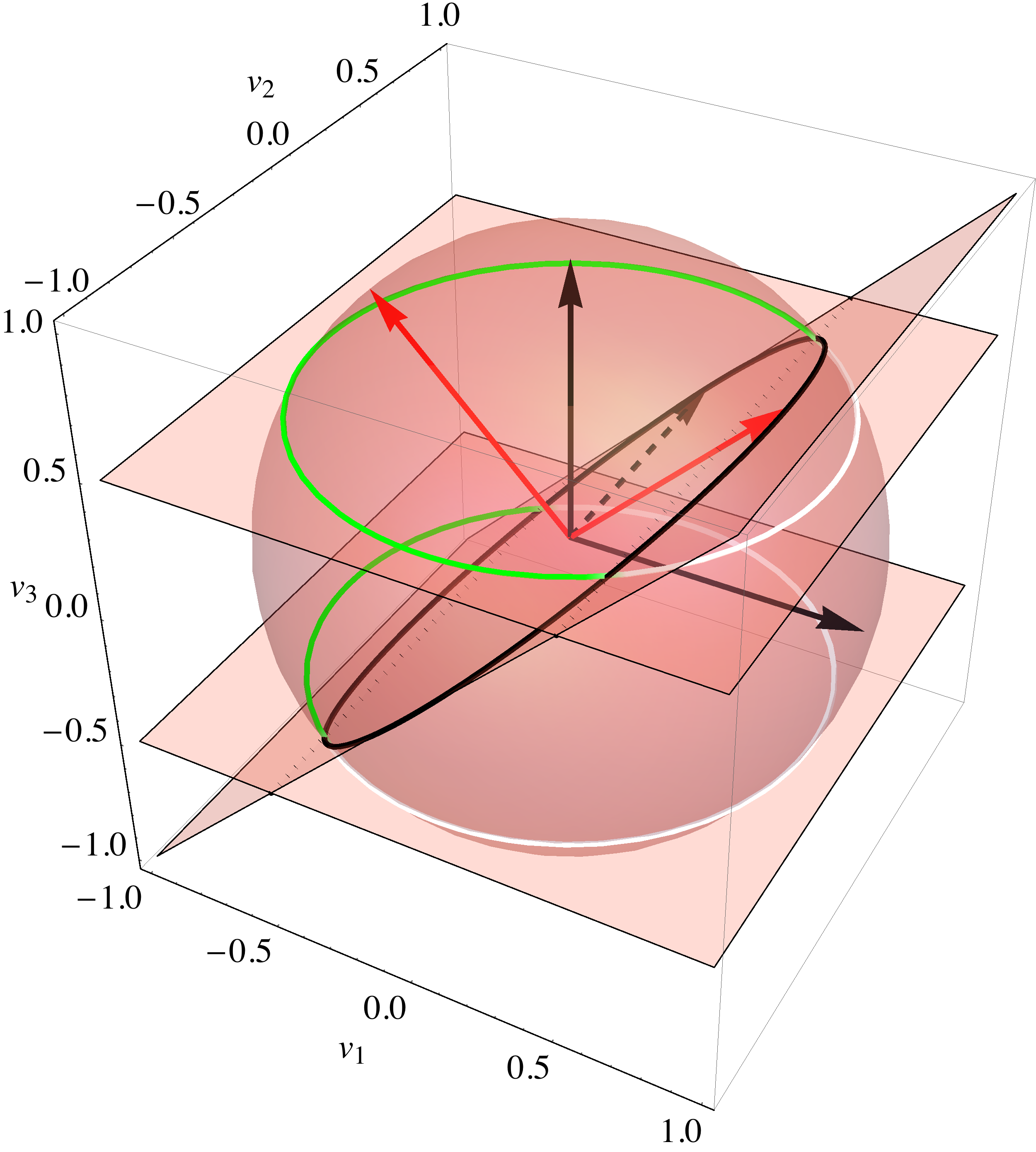
Figure 6: Equation (C.2) has either one ($1/4\leq\epsilon_{\textsc{p}}\leq\tfrac{1}{2}$) or two ($0\leq\epsilon_{\textsc{p}}<1/4$) contributions, given by the integrals along the arc-circles on the hemisphere of velocity coordinates whose projection along the normal to the collision surface (6) is positive. Here $\epsilon_{\textsc{p}}=1/8$ and the two arc-circles at $v_{3}=\pm\tfrac{1}{2}$ contributing to equation (C.2) are the portions (in green) of the corresponding full circles above the plane tangent to the collision surface (the excluded parts of those circles are shown in white).

On the one hand, when the piston’s energy is less than the ball’s, the condition $\sqrt{2\epsilon_{\textsc{p}}}\geq\sqrt{1-2\epsilon_{\textsc{p}}}\cos\alpha$ in the first of the two integrals on the right-hand side of equation (C.2) is equivalent to

$$\arccos\sqrt{\frac{\epsilon_{\textsc{p}}}{\tfrac{1}{2}-\epsilon_{\textsc{p}}}}\leq\alpha\leq 2\pi-\arccos\sqrt{\frac{\epsilon_{\textsc{p}}}{\tfrac{1}{2}-\epsilon_{\textsc{p}}}}\,.$$ (C.3)

Performing the integral, we obtain the contribution,

$$\frac{1}{\sqrt{2}}\int_{\mathbb{S}^{1}:\,\sqrt{2\epsilon_{\textsc{p}}}\geq\sqrt{1-2\epsilon_{\textsc{p}}}\cos\alpha} \mathrm{d}\alpha\,(\sqrt{2\epsilon_{\textsc{p}}}-\sqrt{1-2\epsilon_{\textsc{p}}}\cos\alpha)$$ (C.4)

$$=2\sqrt{\epsilon_{\textsc{p}}}\left(\pi-\arccos\sqrt{\frac{\epsilon_{\textsc{p}}}{\tfrac{1}{2}-\epsilon_{\textsc{p}}}}\right)+2\sqrt{\tfrac{1}{2}-2\epsilon_{\textsc{p}}}\,.$$ (C.5)

Likewise, the condition $\sqrt{2\epsilon_{\textsc{p}}}\leq-\sqrt{1-2\epsilon_{\textsc{p}}}\cos\alpha$ in the second of the two integrals on the right-hand side of equation (C.2) is equivalent to

$$\pi-\arccos\sqrt{\frac{\epsilon_{\textsc{p}}}{\tfrac{1}{2}-\epsilon_{\textsc{p}}}}\leq\alpha\leq\pi+\arccos\sqrt{\frac{\epsilon_{\textsc{p}}}{\tfrac{1}{2}-\epsilon_{\textsc{p}}}}\,.$$ (C.6)

Thus the second integral yields the contribution

$$\frac{1}{\sqrt{2}}\int_{\mathbb{S}^{1}:\,\sqrt{2\epsilon_{\textsc{p}}}\leq-\sqrt{1-2\epsilon_{\textsc{p}}}\cos\alpha} \mathrm{d}\alpha\,(-\sqrt{2\epsilon_{\textsc{p}}}-\sqrt{1-2\epsilon_{\textsc{p}}}\cos\alpha)$$ (C.7)

$$=-2\sqrt{\epsilon_{\textsc{p}}}\arccos\sqrt{\frac{\epsilon_{\textsc{p}}}{\tfrac{1}{2}-\epsilon_{\textsc{p}}}}+2\sqrt{\tfrac{1}{2}-2\epsilon_{\textsc{p}}}\,.$$ (C.8)

The contribution to equation (23) from the velocity integral in the corresponding energy interval is thus given by the sum of equations (C.5) and (C.8).

On the other hand, when the piston’s energy is larger than the ball’s, the condition $\sqrt{2\epsilon_{\textsc{p}}}\geq\sqrt{1-2\epsilon_{\textsc{p}}}\cos\alpha$ in the first of the two integrals on the right-hand side of equation (C.2) holds true for all angles $\alpha$. The result of the integration,

$$\frac{1}{\sqrt{2}}\int_{\mathbb{S}^{1}:\,\sqrt{2\epsilon_{\textsc{p}}}\geq\sqrt{1-2\epsilon_{\textsc{p}}}\cos\alpha}\mathrm{d}\alpha\,(\sqrt{2\epsilon_{\textsc{p}}}-\sqrt{1-2\epsilon_{\textsc{p}}}\cos\alpha)=2\pi\sqrt{\epsilon_{\textsc{p}}}\,,$$ (C.9)

yields the only contribution to the velocity integral in equation (23).

- (1) D. Ruelle, Physics Letters A 245(3-4), 220 (1998). URL http://dx.doi.org/10.1016/S0375-9601(98)00419-8
- (2) D. Ruelle, in Probabilistic and thermodynamic aspects of nonlinear dynamics, ed. by G. Nicolis (Université Libre de Bruxelles, Brussels, Belgium, 1998). Satellite Meeting to STATPHYS 20.
- (3) J. Fourier, Theorie analytique de la chaleur, par M. Fourier (Firmin Didot, père et fils, 1822). URL http://www.gabay-editeur.com/FOURIER-Theorie-analytique-de-la-chaleur-1822. Reprinted (J Gabay, Paris, 1988)
- (4) F. Bonetto, J.L. Lebowitz, L. Rey-Bellet, Fourier’s Law: a Challenge to Theorists (Imperial College Press, London, 2000), chap. 8, pp. 128–150. URL http://www.worldscientific.com/doi/abs/10.1142/9781848160224_0008. Distributed by World Scientific Publishing Co.
- (5) T.N. Narasimhan, Reviews of Geophysics 37(1), 151 (1999). URL http://dx.doi.org/10.1029/1998RG900006
- (6) S. Lepri, R. Livi, A. Politi, Physics Reports 377, 1 (2003). URL http://dx.doi.org/10.1016/S0370-1573(02)00558-6
- (7) A. Dhar, Advances in Physics 57(5), 457 (2008). URL http://dx.doi.org/10.1080/00018730802538522
- (8) L.A. Bunimovich, C. Liverani, A. Pellegrinotti, Y.M. Suhov, Communications in Mathematical Physics 146, 357 (1992). URL http://dx.doi.org/10.1007/BF02102633
- (9) P. Gaspard, T. Gilbert, Physical Review Letters 101(2), 20601 (2008). URL http://dx.doi.org/10.1103/PhysRevLett.101.020601
- (10) M. Sasada, Heat conductivity for stochastic exchange model with mechanical origin (2015). Preprint
- (11) P. Gaspard, T. Gilbert, Journal of Statistical Mechanics 11(1), 021 (2008). URL http://dx.doi.org/10.1088/1742-5468/2008/11/P11021
- (12) M. Sasada, The Annals of Probability 43(4), 1663 (2015). URL http://dx.doi.org/10.1214/14-AOP916
- (13) A. Grigo, K. Khanin, D. Szász, Nonlinearity 25(8), 2349 (2012). URL http://dx.doi.org/10.1088/0951-7715/25/8/2349
- (14) C. Liverani, S. Olla, Journal of the American Mathematical Society 25(2), 555 (2012). URL http://dx.doi.org/10.1090/S0894-0347-2011-00724-8
- (15) J. Bricmont, A. Kupiainen, Communications in Mathematical Physics 274(3), 555 (2007). URL http://dx.doi.org/10.1007/s00220-007-0284-5
- (16) C. Bernardin, S. Olla, Journal of Statistical Physics 121(3), 271 (2005). URL http://dx.doi.org/10.1007/s10955-005-7578-9
- (17) G. Keller, C. Liverani, Communications in Mathematical Physics 291(2), 591 (2009). URL http://dx.doi.org/10.1007/s00220-009-0835-z
- (18) F. Huveneers, Journal of Statistical Physics 146(1), 73 (2012). URL http://dx.doi.org/10.1007/s10955-011-0374-9
- (19) J.P. Eckmann, L.S. Young, Communications in Mathematical Physics 262(1), 237 (2006). URL http://dx.doi.org/10.1007/s00220-005-1462-y
- (20) Y. Li, P. Nándori, L.S. Young, Journal of Statistical Physics 163(1), 61 (2016). URL http://dx.doi.org/10.1007/s10955-016-1466-3
- (21) C. Kipnis, C. Marchioro, E. Presutti, Journal of Statistical Physics 27(1), 65 (1982). URL http://link.springer.com/article/10.1007/BF01011740
- (22) F. Bonetto, J.L. Lebowitz, J. Lukkarinen, Journal of Statistical Physics 116, 783 (2004). URL http://dx.doi.org/10.1023/B:JOSS.0000037232.14365.10
- (23) P. Gaspard, T. Gilbert, New Journal of Physics 10(1), 3004 (2008). URL http://dx.doi.org/10.1088/1367-2630/10/10/103004
- (24) P. Gaspard, T. Gilbert, Chaos 22, 026117 (2012). URL http://dx.doi.org/10.1063/1.3697689
- (25) P. Bálint, I.P. Tóth, Annales Henri Poincaré 9, 1309 (2008). URL http://dx.doi.org/10.1007/s00023-008-0389-1
- (26) Z. Pajor-Gyulai, D. Szász, I.P. Tóth, in XVIth International Congress on Mathematical Physics. Prague. Held 3-8 August 2009, ed. by P. Exner (World Scientific, 2010), pp. 328–332. URL http://www.worldscientific.com/worldscibooks/10.1142/7727
- (27) N. Chernov, D. Dolgopyat, Brownian Brownian Motion-I, Memoirs of the American Mathematical Society, vol. 198 (American Mathematical Society, 2009). URL http://www.ams.org/bookstore-getitem/item=memo-198-927
- (28) P. Bálint, P. Nándori, D. Szász, I.P. Tóth, Equidistribution for standard pairs in planar dispersing billiard flows (2015). Work in progress.
- (29) D. Dolgopyat, C. Liverani, Communications in Mathematical Physics 308(1), 201 (2011). DOI 10.1007/s00220-011-1317-7. URL http://dx.doi.org/10.1007/s00220-011-1317-7
- (30) D. Dolgopyat, P. Nándori, arXiv preprint arXiv:1603.07590 (2016). URL http://arxiv.org/abs/1603.07590
- (31) S. Kullback, R.A. Leibler, The Annals of Mathematical Statistics 22(1), 79 (1951). URL http://www.jstor.org/stable/2236703
- (32) I.P. Cornfeld, S.V. Fomin, Y.G. Sinai, Ergodic Theory (Springer Verlag, New York Heidelberg Berlin, 1982). URL http://link.springer.com/book/10.1007%2F978-1-4615-6927-5
- (33) N.I. Chernov, Journal of Statistical Physics 88(1–2), 1 (1997). URL http://dx.doi.org/10.1007/BF02508462
- (34) N.I. Chernov, Functional Analysis and Its Applications 25(3), 204 (1991). DOI 10.1007/BF01085490. URL http://dx.doi.org/10.1007/BF01085490
- (35) P. Gaspard, T. Gilbert, Journal of Statistical Mechanics 08(0), 020 (2009). URL http://dx.doi.org/10.1088/1742-5468/2009/08/P08020