Towards Compositional Feedback in Non-Deterministic and Non-Input-Receptive Systems

Abstract

Feedback is an essential composition operator in many classes of reactive and other systems. This paper studies feedback in the context of compositional theories with refinement. Such theories allow to reason about systems on a component-by-component basis, and to characterize substitutability as a refinement relation. Although compositional theories of feedback do exist, they are limited either to deterministic systems (functions) or input-receptive systems (total relations). In this work we propose a compositional theory of feedback which applies to non-deterministic and non-input-receptive systems (e.g., partial relations). To achieve this, we use the semantic frameworks of predicate and property transformers, and relations with fail and unknown values. We show how to define instantaneous feedback for stateless systems and feedback with unit delay for stateful systems. Both operations preserve the refinement relation, and both can be applied to non-deterministic and non-input-receptive systems.

1 Introduction

Large and complex systems are best designed using component-based rather than monolithic methodologies. In the component-based paradigm a system is an assembly of interacting components. Each component can itself be a subsystem composed from other components. Arbitrary component hierarchies can be built in this manner, allowing to decompose a complex system into simpler and further simpler subsystems.

Systems constantly evolve, and a key concern in a component-based setting is substitutability: when can we replace some component $A$ with a new component $A^{\prime}$? The issue is property preservation: the replacement must not result in breaking essential properties of the existing system. Moreover, we would like to avoid as much as possible having to re-verify the new system from scratch, since verification is an expensive process. Ideally, a simple check should suffice to guarantee that the new system is correct, assuming that the old system was correct.

Compositional theories with refinement provide an elegant framework for reasoning about these problems. In such theories the following notions are central: (a) the notion of component; (b) composition operators, which create new components by composing existing ones; (c) the notion of refinement, which is a binary relation between components. Typically two main theorems are provided by such a theory:

1. Preservation of refinement by composition, which can be roughly stated as: if $A^{\prime}$ refines $A$ and $B^{\prime}$ refines $B$, then the composition of $A^{\prime}$ and $B^{\prime}$ refines the composition of $A$ and $B$.

2. Preservation of properties by refinement, which can be roughly stated as: if $A^{\prime}$ refines $A$ and $A$ satisfies property $\phi$, then $A^{\prime}$ also satisfies $\phi$.

To see how the above two theorems can be used, consider again the scenario above where $A$ is replaced by $A^{\prime}$. We can avoid re-verifying the new system by trying instead to show that $A^{\prime}$ refines $A$. If this is true, then by preservation of refinement by composition it follows that the new system (with $A^{\prime}$) refines the old system (with $A$). (Here we also implicitly use that refinement is reflexive, which is typically true.) Moreover, by preservation of properties by refinement it follows that if property $\phi$ holds in the old system then it will also hold in the new system. In this way, we can avoid checking $\phi$ directly on the new system, which can be expensive when the system is large. Instead, we must show that $A^{\prime}$ refines $A$, which is an easier verification problem, as it deals with only two components.

In this paper we look at components as blocks with inputs and outputs. In such a setting, there are three basic composition operators (see Figure 1):

Figure 1: Composition operators: serial composition (left); parallel composition (middle); feedback composition (right).

• Serial composition, where the output of one component is connected to the input of another component.

• Parallel composition, where two components are “stacked on top of each other” without any connections, but encapsulated into a single component.

• Feedback composition, where the output of a component is connected into one of its inputs.

Semantically, we want our components to be able to model systems which are both non-deterministic and non-input-receptive. Non-determinism means that the system may produce more than one output for a given input. Non-determinism is well established as a powerful modeling mechanism which allows abstracting from unnecessary details among other things. Non-input-receptiveness means that the system may declare some input values to be illegal (always, or at certain times). For example, a component computing the square root of a real number may declare that negative inputs are illegal. Note that this is different from stating that if the input is negative then the output can be arbitrary. The latter corresponds logically to an implication: $x\geq 0\Rightarrow y=\sqrt{x}$ (here $x$ denotes the input and $y$ the output); whereas the former corresponds to a conjunction: $x\geq 0\land y=\sqrt{x}$. Although less common in the domains of formal methods and verification, non-input-receptive systems are common in programming languages and type theory, where they provide the basis for type checking. Type checking is a key feature of many languages and can be seen as a “lightweight” verification mechanism as the programmer does not have to provide a formal specification of her program (the program only needs to type check). In our setting, non-input-receptiveness is essential in order to be able to model compatibility of components during composition. For an extensive discussion of this point, see [dA04, TLHL11].

In this setting, parallel composition is relatively straightforward to define and can be logically seen as taking the conjunction of the specifications of the two components. Serial composition is a bit trickier and logically involves $\forall$-$\exists$ quantification, which essentially states that any output of the upstream component is a legal input for the downstream component (i.e., there exists for it an output of the downstream component). This game theoretic semantics is necessary when the components are both non-deterministic and non-input-receptive, while it collapses to the standard semantics (composition of functions or relations, or logical conjunction) when components are either deterministic or input-receptive [dA04, dAH01, TLHL11]. Both parallel and serial composition as defined above are compositional in the sense that they preserve refinement.

Compositional theories of feedback do exist, but they are limited to either deterministic systems, or to input-receptive systems. To our knowledge, compositional feedback for both non-deterministic and non-input-receptive systems has so far remained elusive. The main difficulty has been to come up with a definition of feedback which preserves refinement. That is, if $A^{\prime}$ refines $A$, then $\kappa(A^{\prime})$ refines $\kappa(A)$, where $\kappa(\cdot)$ is the feedback composition operator. An extensive account of some of the difficulties and failed attempts is given in [TS14], for the framework of relational interfaces [TLHL11].

To illustrate some of the earlier problems and how they are handled in the new framework, consider the following example, first given in [DHJP08]. Let $A$ be a component with two input variables $u,x$, one output variable $v$, and input-output relation $\mathsf{true}$, which means that $A$ accepts any input value, and given an input value, it can return any output (because $\mathsf{true}$ is satisfied by any $(u,x,v)$ triple). Now let $A^{\prime}$ be another component with inputs $u,x$, output $v$, and relation $u\neq v$. This means that $A^{\prime}$ accepts any input $(u,x)$, and given such $u$, returns some $v$ different from $u$. In the relational interface framework (as well as in our framework), $A^{\prime}$ refines $A$. This is because $A^{\prime}$ has the same legal inputs as $A$ (in fact, every input is legal for both) and $A^{\prime}$ is “more deterministic” than $A$.

Now, suppose we apply feedback to both $A$ and $A^{\prime}$, in particular, we connect output $v$ to input $u$. Denote the resulting components by $B$ and $B^{\prime}$, respectively. Both $B$ and $B^{\prime}$ have a single input, $x$ ($u$ is no longer a free input, since it has been connected to $v$). What should the relations of $B$ and $B^{\prime}$ be? Note that we want $B^{\prime}$ to refine $B$, otherwise refinement is not preserved by feedback. The straightforward way to define feedback is to add the constraint $u=v$, since $v$ is connected to $u$, essentially becoming the same “wire”. Doing so, we obtain $\mathsf{true}\land u=v$, i.e., $u=v$, as the relation of $B$, and $u\neq v\land u=v$, i.e., $\mathsf{false}$, as the relation of $B^{\prime}$. This is problematic, since $\mathsf{false}$ does not refine $u=v$. Indeed, according to the game-theoretic semantics, refinement is not implication, because inputs and outputs must be treated differently. In our example, any input $x$ is legal for $B$, whereas no input $x$ is legal for $B^{\prime}$, which means that $B^{\prime}$ cannot replace $B$, i.e., does not refine it.

In this paper, we attack the problem of feedback afresh. We adopt the frameworks of refinement calculus (RC) [BvW98] and refinement calculus of reactive systems (RCRS) [PT14]. RC is a classic compositional framework for reasoning about sequential programs, while RCRS is an extension of RC to reason about reactive systems. In RC, programs are modeled as (monotonic) predicate transformers, i.e., functions from sets of post-states to sets of pre-states. In RCRS, systems are modeled as (monotonic) property transformers, which are functions that transform sets of output infinite sequences into sets of input infinite sequences. Both predicate and property transformers are powerful mathematical tools, able to capture both non-deterministic and non-input-receptive systems. In fact, they are more powerful than partial relations, which is the semantic basis of relational interfaces [TLHL11]. Therefore one can hope that some of the difficulties in obtaining a compositional definition of feedback in the relational framework can be overcome in the refinement calculi frameworks.

We first consider stateless systems and instantaneous feedback, i.e., feedback in a single step (Section 5). We model stateless systems using predicate transformers, where instead of a post/pre-state interpretation, we use an output/input interpretation. We often employ strictly conjunctive predicate transformers, which correspond to input-output relations over a domain extended with a special value fail (denoted $\bullet$), used to model illegal inputs (those return $\bullet$ as output). We further extend these relations with an additional unknown value (denoted $\bot$). The unknown value is used to define feedback by means of a fix-point iteration, starting with unknown and potentially converging to known values. The idea to use unknown values and fix-points comes from methods for dealing with instantaneous feedback in deterministic and input-receptive systems (i.e., total functions) [Mal94, Ber99, EL03]. In our case systems are non-deterministic and also may reject some inputs. We therefore need to generalize the fix-point method to relations with fail and unknown. The precise definition is involved (Def. 2), but roughly speaking, for a given input we explore all possible computation paths, including those in which the feedback input stabilizes to a known or unknown value, as well as those in which either the relation returns $\bullet$ or the path does not stabilize. We can then consider an input to the post-feedback system as legal if no execution path fails, and those which stabilize reach a known value.

This instantaneous feedback operator preserves refinement. In the example discussed above, the new definition results in both $B$ and $B^{\prime}$ being the component $\mathsf{Fail}$ which rejects all inputs, since the above procedure does not stabilize in neither the case of $A$ nor $A^{\prime}$. This indicates that the two feedback operations are illegal, which is similar to discovering an incompatibility during, say, serial composition.

Relations with fail and unknown have the same modeling power as strictly conjunctive predicate transformers over input/output values with unknowns. We use the two models alternatively, as each is best suited to obtain certain results. In particular, we define the instantaneus feedback operator using relations with fail and unknowns, but we prove that the operator preserves refinement using their predicate transformer representation.

We next turn to the case of stateful systems. Syntactically, we model these as symbolic transition systems, i.e., relations on input, output, current state, and next state variables. For instance, a simple counter can be modeled by the relation $u^{\prime}=u+1$, where $u$ denotes the current state and $u^{\prime}$ the next state. Semantically, we use predicate transformers on the same variables [PT14]. We then define feedback with unit-delay for such predicate transformers, which corresponds to connecting $u^{\prime}$ to $u$ via a unit-delay component. A unit-delay outputs at step $k$ its input at the previous step $k-1$. Thus, feedback with unit-delay ensures that the next state $u^{\prime}$ becomes the current state in the next step. The feedback with unit-delay operator is defined in Section 7. That definition is aided by iteration operators over property transformers defined in Section 6.

Combining the two feedback operators generalizes block-diagram languages like Simulink, which are not able to handle non-deterministic and non-input-receptive components.

Our treatment in this paper is mostly semantic. However, following [PT14], we can use syntactic objects such as symbolic transition systems to represent predicate and property transformers. For example, the formula $u^{\prime}=u+1$ represents a counter, as mentioned above; the formula $x\geq 0\land y=\sqrt{x}$, where $x$ is input and $y$ is output, represents a relation with fail and also a predicate transformer. We can also use temporal logic (e.g., LTL [Pnu77]) to express properties over infinite sequences of input-output values, including liveness properties. For example, a system specified by the LTL formula $\Box\,(x\Rightarrow\Diamond\,y)$ ensures that if the input $x$ is infinitely often true, so will be the output $y$. Using these representations, most of the constructs presented in this paper can actually be computed as first-order formulas, or as quantified LTL formulas.

All the results presented in this paper have been formalized and proved in the Isabelle theorem prover [NPW02]. The Isabelle code is available from http://rcrs.cs.aalto.fi.

2 Related Work

Our idea to use relations with an unknown value is inspired from fix-point based methods such as constructive semantics, which are used to reason about instantaneous feedback in cyclic combinational circuits and synchronous languages [Mal94, Ber99, EL03]. These methods deal with monotonic functions over the flat CPO with unknown as the least element. Because they assume total functions, they are limited to deterministic and input-receptive systems. Refinement is also absent from these frameworks.

Fix-point based methods have also been used to reason about non-instantaneous feedback, in systems such as Kahn Process Networks [Kah74], where processes are modeled as continuous functions on streams. Again, these are total functions, and therefore deterministic and input-receptive. Non-deterministic extensions of process networks exist [Jon94] but they do not include a notion of refinement.

Frameworks which allow non-determinism and also include refinement are I/O automata [LT89], reactive modules [AH99], and Focus [BS01]. All three frameworks assume that components are input-receptive. Note that in the example given in the introduction, although components $A$ and $A^{\prime}$ are input-receptive, and so is $B$, $B^{\prime}$ is not. This shows that the straightforward definition of feedback does not preserve input-receptiveness. It is unclear how this example could be handled in the above frameworks.

Interface automata [dAH01] allow non-deterministic as well as non-input-receptive specifications. Composition in this framework is asynchronous parallel composition with input-output label synchronization, and therefore difficult to directly compare with feedback composition in our framework. Also, interface automata are limited to safety whereas our framework can also express liveness properties.

Checking compatibility within the framework of functional programing languages, can be done using type-checking as in the Standard ML language [MTH90], or using more advanced techniques as Refinement Types for ML [FP91], Dependent Types [XP99], and Liquid Types [RKJ08]. These are techniques based on subtypes and dependent-types that allow checking at compile time of invariants about the computed values of the program. These techniques are in general automated, therefore they are applicable only to certain classes of decidable problems. Our compatibility check for system compositions is more general, and not necessarily decidable. In our case checking compatibility of system compositions is reduced to checking satisfiability of formulas. If the underlying logic of these formulas is decidable, then we can have an automatic compatibility test.

In [Mil90] a model for synchronous nondeterministic systems is used for studying preservation of security properties by composition of systems, including delayed feedback. However this model does not treat non-input receptive systems.

3 Background

We use higher order logic as implemented by the Isabelle theorem prover. Capital letters $X,Y,\ldots$ denote types and small letters denote elements of these types $x\in X$. $\mathsf{Bool}$ denotes the type of Boolean values $\mathsf{true}$ and $\mathsf{false}$, $\mathsf{Nat}$ the natural numbers, and $\mathsf{Real}$ the reals. We use $\land$, $\lor$, $\Rightarrow$, and $\neg$ for the Boolean operations.

If $X$ and $Y$ are types, then $X\to Y$ denotes the type of function from $X$ to $Y$. For function application we use a dot notation. If $f:X\to Y$ is a function, and $x\in X$, then $f.x$ is the function $f$ applied to $x$. The function type constructor associates to right, and correspondingly the function application associates to left. That is $X\to Y\to Z$ is the same as $X\to(Y\to Z)$ and $f.x.y$ is the same as $(f.x).y$. We also use lambda abstraction to construct functions. For example if $x+2\cdot y\in\mathsf{Nat}$ is natural expression, then $(\lambda x,y:x+2\cdot y):\mathsf{Nat}\to\mathsf{Nat}\to\mathsf{Nat}$ is the function that maps $x$ and $y$ into $x+2\cdot y$. We use the notation $X\times Y$ for the Cartesian product of $X$ and $Y$ and if $x\in X$ and $y\in Y$, then $(x,y)$ denotes the pair of $x$ and $y$ from $X\times Y$.

Predicates are functions with one or more arguments returning Booleans (e.g., a predicate with two arguments has signature $X\to Y\to\mathsf{Bool}$), and relations are predicates with at least two arguments. For a relation $r:X\to Y\to\mathsf{Bool}$ we denote by $\mathsf{in}.r:X\to\mathsf{Bool}$ the predicate given by $\mathsf{in}.r.x=(\exists y:r.x.y)$. If $r$ is a relation with more than two arguments, then $\mathsf{in}.r$ is defined similarly by quantifying over the last argument: $\mathsf{in}.r.x.y.z=(\exists u:r.x.y.z.u)$.

We extend point-wise all operations on Booleans to operations on predicates and relations. For example if $r,r^{\prime}:X\to Y\to\mathsf{Bool}$ are two relations then $r\land r^{\prime}$ and $r\lor r^{\prime}$ are the relations given by $(r\land r^{\prime}).x.y=r.x.y\land r^{\prime}.x.y$ and $(r\lor r^{\prime}).x.y=r.x.y\lor r.x.y$, and $(r\leq r^{\prime})=(\forall x,y:r.x.y\Rightarrow r^{\prime}.x.y)$. We use $\bot$ and $\top$ as the smallest and greatest predicates (relations): $\bot.x=\mathsf{false}$ and $\top.x=\mathsf{true}$.

For relations $r:X\to Y\to\mathsf{Bool}$ and $r^{\prime}:Y\to Z\to\mathsf{Bool}$, we denote by $r\circ r^{\prime}$ the relational composition given by $(r\circ r^{\prime}).x.z=(\exists y:r.x.y\land r^{\prime}.y.z)$. For a relation $r:X\to Y\to\mathsf{Bool}$ we denote by $r^{-1}:Y\to X\to\mathsf{Bool}$ the inverse of $r$ ($r^{-1}.y.x\Leftrightarrow r.x.y$). A relation $r$ is total (sometimes called left-total) if for all $x$ there is $y$ such that $r.x.y$.

For reactive systems we need infinite sequences (or traces) of values. Formally, if $X$ is a type of values, then a trace from $X$ is an element $\mathbf{x}\in X^{\omega}=(\mathsf{Nat}\to X)$. To make the reading easier, we denote infinite sequences by bold face letters $\mathbf{x},\mathbf{y},\ldots$ and values by normal italic small letters $x,y,\ldots$. When, for example, both $x$ and $\mathbf{x}$ occur in some formula, we use the convention that the elements of $\mathbf{x}$ have the same type as $x$. For $\mathbf{x}\in X^{\omega}$, $\mathbf{x}_{i}=\mathbf{x}.i$, and $\mathbf{x}^{i}\in X^{\omega}$ is given by $\mathbf{x}_{j}^{i}=\mathbf{x}^{i}.j=\mathbf{x}_{i+j}$. We consider a pair of traces $(\mathbf{x},\mathbf{y})$ as being the same as the trace of pairs $(\lambda i:(\mathbf{x}_{i},\mathbf{y}{}_{i}))$.

3.1 Linear temporal logic

Linear temporal logic (LTL) [Pnu77] is a logic used for specifying properties of reactive systems. In this paper we use a semantic (algebraic) version of LTL as in [PT14]. This logic is formalized in Isabelle, and the details of this formalization are available in [Pre14]. An LTL formula is a predicate on traces and the temporal operators are functions mapping predicates to predicates. We call predicates over traces (i.e., sets of traces) properties.

If $p,\;q\in X^{\omega}\to\mathsf{Bool}$ are properties, then always $p$, next $p$, and $p$ until $q$ are also properties and they are denoted by $\Box\,p$, $\fullmoon\,p$, and $p\;\mathsf{U}\;q$ respectively. The property $\Box\,p$ is true in $\mathbf{x}$ if $p$ is true at all time points in $\mathbf{x}$, $\fullmoon\,p$ is true in $\mathbf{x}$ if $p$ is true at the next time point in $\mathbf{x}$, and $p\;\mathsf{U}\;q$ is true in $\mathbf{x}$ if there is some time in $\mathbf{x}$ when $q$ is true, and until then $p$ is true. Formally we have:

$$\begin{array}[]{l}(\Box\,p).\mathbf{x}=(\forall n:p.\mathbf{x}^{n}),\ \ (\fullmoon\,p).\mathbf{x}=p.\mathbf{x}^{1}\\ (p\;\mathsf{U}\;q).\mathbf{x}=(\exists n:(\forall i<n:p.\mathbf{x}^{i})\land q.\mathbf{x}^{n})\end{array}$$

In addition we define the operator $p\mathsf{\,L\,}q=\neg(p\;\mathsf{U}\;\neg q)$. Intuitively, $p\mathsf{\,L\,}q$ holds if, whenever $p$ holds continuously up to step $n-1$, then $q$ must hold at step $n$.

If $r$ is a relation on traces we define the temporal operators similarly. For example $(\Box\,r).\mathbf{x}.\mathbf{y}.\mathbf{z}=(\forall n:r.\mathbf{x}^{n}.\mathbf{y}^{n}.\mathbf{z}^{n})$. If $r$ is a relation on values, then we extend it to traces by $r.\mathbf{x}.\mathbf{y}.\mathbf{z}=r.\mathbf{x}_{0}.\mathbf{y}_{0}.\mathbf{z}_{0}$.

3.2 Refinement calculus of reactive systems

In refinement calculus programs are modeled as monotonic predicate transformers [BvW98]. A program $S$ with input type $X$ and output type $Y$ is modeled as a function from $(Y\to\mathsf{Bool})\to(X\to\mathsf{Bool})$ with a weakest precondition interpretation. If $q:Y\to\mathsf{Bool}$ is a post-condition (set of final states), then $S.q$ is the set of all initial states from which the program always terminates and it terminates in a state from $q$. We model reactive systems as monotonic property transformers, also with a weakest precondition interpretation [PT14]. A reactive system $S$ with input type $X$ and output type $Y$ is formally modeled as a monotonic function from $(Y^{\omega}\to\mathsf{Bool})\to(X^{\omega}\to\mathsf{Bool})$. If $q:Y^{\omega}\to\mathsf{Bool}$ is a post-property (a set of output traces), then $S.q$ is the set of input traces for which the execution of $S$ does not fail and it produces an output trace in $q$. The remaining of this section applies equally to both monotonic predicate transformers and monotonic property transformers, and we will call them simply monotonic transformers.

The point-wise extension of the Boolean operations to predicates, and then to monotonic transformers gives us a complete lattice with the operations $\sqsubseteq$, $\sqcap,\;\sqcup,\ \bot,\;\top$ (observe that $\sqcap$ and $\sqcup$ preserve monotonicity). All these lattice operations are also meaningful as operations on programs and reactive systems. The order of this lattice ($S\sqsubseteq T\Leftrightarrow(\forall q:S.q\leq T.q)$) is the refinement relation. If $S\sqsubseteq T$, then we say that $T$ refines $S$ (or $S$ is refined by $T$). If $T$ refines $S$ then $T$ can replace $S$ in any context.

The operations $\sqcap$ and $\sqcup$ model demonic and angelic non-determinism or choice. The interpretation of $\sqcap$ is that the system $S\sqcap T$ is correct (i.e., satisfies its specification) if both $S$ and $T$ are correct. On the other hand $S\sqcup T$ is correct if one of $S$ and $T$ are correct. Thus, $\sqcap$ and $\sqcup$ represent uncontrollable and controllable non-determinism, respectively.

We denote the bottom and the top of the lattice of monotonic transformers by $\mathsf{Fail}$ and $\mathsf{Magic}$ respectively. $\mathsf{Fail}$ is refined by any monotonic transformer and $\mathsf{Magic}$ refines every monotonic transformer. $\mathsf{Fail}$ does not guarantee any property. For any $q$, $\mathsf{Fail}.q=\bot$, i.e., there is no input (sequence) for which $\mathsf{Fail}$ will produce an output (sequence) from $q$. On the other hand $\mathsf{Magic}$ can establish any property $q$ ($\mathsf{Magic}.q=\top$). The problem with $\mathsf{Magic}$ is that it cannot be implemented.

Serial composition of two systems modeled as transformers $S$ and $T$ is simply the functional composition of $S$ and $T$ ($S\circ T$). For monotonic transformers we denote this composition by $S\;;\,T$ ($(S\;;\,T).q=S.(T.q)$). To be able to compose $S$ and $T$, the type of the output of $S$ must be the same as the type of the input of $T$.

The system $\mathsf{Skip}$ defined by $(\forall q:\mathsf{Skip}.q=q)$ is the neutral element for serial composition:

$$\mathsf{Skip}\;;\,S=S\;;\,\mathsf{Skip}=S.$$

We now define two special types of monotonic transformers which will be used to form more general property transformers by composition. For predicate $p:X\to\mathsf{Bool}$ and relation $r:X\to Y\to\mathsf{Bool}$ we define the assert transformer $\{p\}:(X\to\mathsf{Bool})\to(X\to\mathsf{Bool})$, and the demonic update transformer $[r]:(Y\to\mathsf{Bool})\to(X\to\mathsf{Bool})$ as follows:

$$\{p\}.q=(p\land q),\ \ \ \ \ [r].q.x=(\forall y:r.x.y\Rightarrow q.y)$$

The assert system $\{p\}$ when executed from a sequence $x$, behaves as skip when $p.x$ is true, and it fails otherwise. The demonic update statement $[r]$ establishes a post condition $q$ when starting in $x$ if all $y$ with $r.x.y$ are in $q$. If $r=\bot$, then $[r]=[\bot]=\mathsf{Magic}$.

If $R$ is an expression in $x$ and $y$, then $[x\leadsto y\;|\;R]=[\lambda x,y:R]$. For example if $R$ is $z=x+y$, then $[x,\;y\leadsto z\;|\;z=x+y]=[\lambda(x,\;y),\;z:z=x+y]$ is the system which produces in the output $z$ the value $x+y$ where $x$ and $y$ are the inputs. If $e$ is an expression in $x$, then $[x\leadsto e]=[x\leadsto y\;|\;y=e]$, where $y$ is a new variable different of $x$ and which does not occur free in $e$. For assert statements we introduce similar notation. If $P$ is an expression in $x$ then $\{x\;|\;P\}=\{\lambda x:P\}$. If $P$ is $x\leq y$, then $\{x,\;y\;|\;x\leq y\}=\{\lambda(x,y):x\leq y\}$. The variables $x$ and $y$ are bounded in $[x\leadsto y\;|\;R]$ and $\{x\;|\;P\}$.

The havoc monotonic transformer is the most non-deterministic statement $\mathsf{Havoc}=[x\leadsto y\;|\;\mathsf{true}]$ and it assigns some arbitrary value to the output $y$.

In RCRS we can model (global) specifications of reactive systems, e.g., using LTL as a specification language, as well as concrete implementations, e.g., using symbolic transition systems (relations on input, output, state, and next-state variables) [PT14]. A global specification may define what the output of a system is when the input is an entire sequence $\mathbf{x}$. A global specification may also impose conditions on the entire input sequence $\mathbf{x}$, including liveness conditions. For example, the formula $\Box\,\Diamond\,x$ asserts that the input must be true infinitely often. An implementation describes how the system works step-by-step. For instance, an implementation may start with input $\mathbf{x}_{0}$ and some initial internal state $\mathbf{u}_{0}$, compute the output $\mathbf{y}_{0}$ and a new internal state $\mathbf{u}_{1}$, and then use $\mathbf{x}_{1}$ and $\mathbf{u}_{1}$ to compute $\mathbf{y_{1}}$ and $\mathbf{u}_{2}$, and so on.

Example 1 (System modeling with property and predicate transformers).

We can model a global reactive system $\mathit{Sum}$ that for every input sequence $\mathbf{x}\in\mathsf{Nat}^{\omega}$ computes the sequence $sum.\mathbf{x}\in\mathsf{Nat}^{\omega}$, where $sum.\mathbf{x}.n=\mathbf{x}_{0}+\mathbf{x}_{1}+\ldots+\mathbf{x}_{n-1}$. We model $\mathit{Sum}$ as a monotonic property transformer:

$$\mathit{Sum}=[\mathbf{x}\leadsto sum.\mathbf{x}]$$

We can also model a step of an implementation of $\mathit{Sum}$ as a predicate transformer:

$$\mathit{StepSum}=[u,x\leadsto u^{\prime},y\;|\;u^{\prime}=u+x\land y=u]$$ (1)

The relation $u^{\prime}=u+x\land y=u$ describes a symbolic transition system: $u$ is the current state, $u^{\prime}$ the next state, $x$ is the input, and $y$ the output. $\mathit{StepSum}$ works iteratively starting at initial state $\mathbf{u}_{0}$, and the first element of the input $\mathbf{x}$, and assuming that $\mathbf{u}_{0}=0$, it computes $\mathbf{u}_{1}=\mathbf{u}_{0}+\mathbf{x}_{0}=\mathbf{x}_{0}$ and $\mathbf{y}_{0}=\mathbf{u}_{0}=0=sum.\mathbf{x}.0$, then using $\mathbf{u}_{1}$ and second element $\mathbf{x}_{1}$ of $\mathbf{x}$, it computes $\mathbf{u}_{2}=\mathbf{u}_{1}+\mathbf{x}_{1}=\mathbf{x}_{0}+\mathbf{x}_{1}$ and $\mathbf{y}_{1}=\mathbf{u}_{1}=\mathbf{x}_{0}=sum.\mathbf{x}.1$, and so on. We will show later in Example 13 how to obtain the $\mathit{Sum}$ property transformer by connecting in $\mathit{StepSum}$ the output $u^{\prime}$ to the input $u$ in feedback with a unit delay.

The assert and demonic choice predicate transformers satisfy the following properties [BvW98]:

Theorem 1.

For $p,p^{\prime}$ and $r,r^{\prime}$ of appropriate types we have

1. $\{p\}\;;\,[r]\;;\,\{p^{\prime}\}\;;\,[r^{\prime}]=\{x\;|\;p.x\land\forall y:r.x.y\Rightarrow p^{\prime}.y\}\;;\,[r\circ r^{\prime}]$

2. $\{p\}\;;\,[r]\sqsubseteq\{p^{\prime}\}\;;\,[r^{\prime}]\Leftrightarrow(\forall x:(p.x\Rightarrow p^{\prime}.x)\land(\forall y:p.x\land r^{\prime}.x.y\Rightarrow r.x.y))$

For a monotonic predicate transformer $S$, the strong and weak iteration of $S$, denoted $S^{\omega}$ and $S^{*}$, are the least and greatest fix-points of $(\lambda X:\mathsf{Skip}\sqcap S\;;\,X)$, respectively. These fix-points exist by the Knaster-Tarski fix-point theorem for monotonic functions on complete lattices [Tar55]. When $S^{*}$ is executed, $S$ is repeated a demonically chosen finite number of times. $S^{\omega}$ is similar, but if $S$ can be executed indefinitely then $S^{\omega}$ fails. $S^{\omega}$ can be used to give semantics to the while statement suitable for total correctness reasoning, while $S^{*}$ can be used to give semantics to the while statement suitable for partial correctness reasoning. In this paper we will use $S^{*}$ to give an alternative definition for the instantaneous feedback operator.

3.3 Product and fusion of monotonic transformers

For two predicates $p$ and $q$ their product is denoted $p\times q$ and is given by

$$(p\times q).(s,s^{\prime})=p.s\land q.s^{\prime}$$

The product (parallel composition) of two monotonic transformers $S$ and $T$ is denoted by $S\times T$ and is given by

$$(S\times T).q.(s,s^{\prime})=(\exists p,r:p\times r\leq q\land S.p.s\land T.r.s^{\prime})$$

If ${\cal{S}}=\{S_{i}\}_{i\in I}$, is a collection of monotonic transformers, then the fusion of $\cal{S}$, denoted $\mathsf{Fusion}.\cal{S}$, is a monotonic transformer given by

$$\mathsf{Fusion}.{\cal S}.q.s=\big{(}\exists p:(\bigwedge_{i\in I}p_{i})\leq q\land(\forall i:S_{i}.p_{i}.s)\big{)}$$

When $\cal S$ contains just two transformers $S$ and $T$, we write $\mathsf{Fusion}(S,T)$ instead of $\mathsf{Fusion}(\{S,T\})$.

Note that product and fusion are similar, but not the same. The result of the product $A\times B$ is a component with separate inputs and outputs for $A$ and $B$ (see Figure 1, parallel composition), whereas the result of $\mathsf{Fusion}(A,B)$ is a component with “shared” input and output.

Theorem 2.

Fusion and product satisfy the following [BB95]

1. $\mathsf{Fusion}.(\{\{p_{i}\}\;;\,[r_{i}]\}_{i\in I})=\{\bigwedge_{i}p_{i\in I}\}\;;\,[\bigwedge_{i\in I}r_{i}]$

2. $S\sqsubseteq S^{\prime}$ and $T\sqsubseteq T$’ implies $S\times T\sqsubseteq S^{\prime}\times T^{\prime}$

3. $(\forall i:S_{i}\sqsubseteq T_{i})$ implies $\mathsf{Fusion}.{\cal S}\sqsubseteq\mathsf{Fusion}.{\cal T}$

4. $(\{p\}\;;\,[r])\times(\{p^{\prime}\}\;;\,[r^{\prime}])=\{x,y\;|\;p.x\land p^{\prime}.y\}\;;\,[x,y\leadsto x^{\prime},y^{\prime}\;|\;r.x.x^{\prime}\land r^{\prime}.y.y^{\prime}]$

3.4 Strictly conjunctive predicate transformers

Dijkstra [Dij75] introduced predicate transformers for reasoning about programs. In addition to monotonicity, he also required some other properties, like conjunctivity ($S.(p\land q)=S.p\land S.q$), and the law of excluded miracle ($S.\bot=\bot$) for his predicate transformers. In this paper we use strictly conjunctive predicate transformers. These are the predicate transformers that satisfy a conjunctivity property stronger than the one used by Dijkstra. A predicate transformer is strictly conjunctive if it commutes with arbitrary non-empty meets:

$$S.(\bigwedge_{i\in I}q_{i})=\bigwedge_{i\in I}S.q_{i}$$

for all nonempty $I$ and $q:I\to Y\to\mathsf{Bool}$.

The set of strictly conjunctive predicate transformers are exactly the predicate transformers of the form $\{p\}\;;\,[r]$, and the set of strictly conjunctive predicate transformers satisfying the law of excluded miracle are exactly the predicate transformers of the form $\{\mathsf{in}.r\}\;;\,[r]$:

Theorem 3.

[BvW98] A predicate transformers $S$ is strictly conjunctive if and only if there exist a predicate $p$ and a relation $r$ such that

$$S=\{p\}\;;\,[r]$$

$S$ is strictly conjunctive and $S$ satisfies the law of excluded miracle, if and only if there exists a relation $r$ such that

$$S=\{\mathsf{in}.r\}\;;\,[r].$$

For instance, for the predicate transformer $\mathsf{Skip}$ we have

$$\mathsf{Skip}=\{\top\}=[x\leadsto x]=\{\top\}\;;\,[x\leadsto x].$$

For the predicate transformers $\{p\}$, $[r]$, $\mathsf{Fail}$ and $\mathsf{Magic}$ we have:

$$\begin{array}[]{lll}\{p\}=\{p\}\;;\,[x\leadsto x]&&\mathsf{Fail}=\{\bot\}=\{\bot\}\;;\,[x\leadsto x]\\[4.30554pt] [r]=\{\top\}\;;\,[r]&&\mathsf{Magic}=[\bot]=\{\top\}\;;\,[\bot]\end{array}$$

Therefore all these transformers are strictly conjunctive, but only $\mathsf{Skip}$, $\{p\}$ and $\mathsf{Fail}$ satisfy the law of excluded miracle. For example we have $\{p\}.\bot=p\land\bot=\bot$. On the other hand $\mathsf{Magic}.\bot=\top$, so $\mathsf{Magic}$ does not satisfy the law of excluded miracle.

Consider also this set of examples:

$$\begin{array}[]{lllllllll}T_{1}&=&[x\leadsto y\;|\;y=x]=[x\leadsto x]&&T_{4}&=&\{x\geq 0\}\;;\,[x\leadsto y\;|\;y=x]\\[4.30554pt] T_{2}&=&[x\leadsto y\;|\;x\geq 0\land y=x]&&T_{5}&=&\{x\geq 0\}\;;\,[x\leadsto y\;|\;x\geq 0\land y=x]\\[4.30554pt] T_{3}&=&[x\leadsto y\;|\;x\geq 0\Rightarrow y=x]&&T_{6}&=&\{x\geq 0\}\;;\,[x\leadsto y\;|\;x\geq 0\Rightarrow y=x]\end{array}$$

All these transformers are strictly conjunctive. $T_{1}$, $T_{2}$, $T_{3}$ and $T_{4}$ are all different. $T_{4}$, $T_{5}$ and $T_{6}$ are all equal because the implication

$$(\forall x,y:p.x\Rightarrow r.x.y=r^{\prime}.x.y)\Rightarrow\{p\}\;;\,[r]=\{p\}\;;\,[r^{\prime}]$$

is valid (i.e., if for any legal input $x$ the outputs of $r$ and $r^{\prime}$ are the same, then the transformers $\{p\}\;;\,[r]$ and $\{p\}\;;\,[r]^{\prime}$ are the same). All inputs are legal for $T_{1}$, $T_{2}$, and $T_{3}$, but only inputs $x\geq 0$ are legal for $T_{4}$. Transformers $T_{1}$, $T_{3}$ and $T_{4}$ satisfy the law of excluded miracle because, for example $\mathsf{in}.(\lambda x,y:x\geq 0\Rightarrow y=x)=\top$ and $T_{3}=\{\mathsf{in}.(\lambda x,y:x\geq 0\Rightarrow y=x)\}\;;\,[x\leadsto y\;|\;x\geq 0\Rightarrow y=x]$. $T_{2}$ does not satisfy the law of excluded miracle because $T_{2}.\bot.x=(x<0)\not=\mathsf{false}$. If we run all $T_{1}$, $T_{2}$, $T_{3}$ and $T_{4}$ on the same input $x\geq 0$, then they all return output $y=x$. However if we run them on the input $x<0$, then they all behave diferently. $T_{1}$ returns output $y=x$. $T_{2}$ behaves magically because the realation $x\geq 0\land y=x$ is false. $T_{3}$ returns some arbitrary $y$ because the relation $x\geq 0\Rightarrow y=x$ is true. $T_{4}$ fails for $x$ because $x$ is an illegal input for $T_{4}$.

For strictly conjunctive predicate transformers the weak iteration is equal to an enumerable demonic choice:

Theorem 4.

If $S$ is strictly conjunctive then

$$S^{*}=\bigsqcap_{n\in\mathsf{Nat}}S^{n}$$

This theorem gives a simpler definition for the weak iteration $S^{*}$ when $S$ is strictly conjunctive, as compared to the case when $S$ is just monotonic. This theorem will be used later in Section 5.2 to connect the definition of instantaneous feedback on relations to the corresponding definition on predicate transformers.

4 Relations with Fail and Unknown

In this section we formally introduce relations with fail and unknown values. As mentioned in the introduction, relations with fail and unknown and strictly conjunctive predicate transformers have the same expressive power, but each is better suited in defining, explaining, or proving certain results.

4.1 Relations with fail

First we introduce relations augmented with a special element $\bullet$ which we call “fail”. These relations are equivalent to strictly conjunctive predicate transformers [BvW98]. If in addition these relations are total, then they are equivalent to predicate transformers that are strictly conjunctive and satisfy the law of excluded miracle [BvW98]. Relations with fail are used in the semantics of imperative programming languages to model non-termination in the context of non-determinism [Plo76]. In this paper $\bullet$ is used to model non-input-receptive systems: when the output is $\bullet$, it means that the input is illegal.

We assume that $\bullet$ is a new element that does not belong to ordinary types. We define the type $A^{\bullet}=A\cup\{\bullet\}$. An element of $x\in A^{\bullet}$ is either $\bullet$ or $x\in A$. An element $x\in(A\times B)^{\bullet}$ is either $\bullet$ or it is a pair $(a,b)$, with $a\in A$ and $b\in B$. A relation with fail from $A$ to $B$ is an element from $A^{\bullet}\to B^{\bullet}\to\mathsf{Bool}$. We assume that relations with fail map $\bullet$ only to $\bullet$, i.e., $R.\bullet.\bullet$ is true, and $R.\bullet.x$ is false for all $x\not=\bullet$. If $R$ is a relation with fail, and $R.x.\bullet$, then $x$ is an illegal input for $R$.

To define a relation with fail $R$, it is enough to define $R.x.\bullet$ for $x\not=\bullet$, and to define $R.x.y$ for $x\not=\bullet$ and $y\not=\bullet$, and we assume also $R.\bullet.\bullet$. Similarly when we state that a relation $R$ has certain properties, we state these two cases, and in addition we also require $R.\bullet.\bullet$.

The condition that relations with fail map $\bullet$ to $\bullet$ is needed to ensure consistency of the serial composition of relations with respect to illegal inputs. For example if $R$ and $R^{\prime}$ are relations with fail of appropriate types, and $x$ is an illegal input for $R$, ($R.x.\bullet$ is true), then $x$ must also be an illegal input for the serial composition $R\circ R^{\prime}$. This is true because $R.x.\bullet$ and $R^{\prime}\bullet.\bullet$ implies $(R\circ R^{\prime}).x.\bullet$.

Example 2 (Division).

$\mathsf{Div}:(\mathsf{Real}^{2})^{\bullet}\to\mathsf{Real}^{\bullet}\to\mathsf{Bool}$ is a relation with fail modeling division:

$$\mathsf{Div}.(x,y).\bullet=(y=0)\mbox{ and }\mathsf{Div}.(x,y).z=(y\not=0\land z=x/y).$$

Because $\mathsf{Div}.(x,0).\bullet$ is true, we have that $(x,0)$ is an illegal input for $\mathsf{Div}$, for any $x$.

If $x$ is an illegal input for $R$, then it is not important if $R$ also maps $x$ to some proper output $y$ ($R.x.y=\mathsf{true}$, with $y\neq\bullet$). If $R^{\prime}$ is a relation almost identical to $R$ except that $R^{\prime}.x.y=\mathsf{false}$, then we consider $R$ and $R^{\prime}$ as modeling the same system. We do not restrict relations with fail to relations that map illegal inputs only to $\bullet$ because we want to model the demonic choice of relations by union. If $R$ and $R^{\prime}$ are of the same type, then $R\vee R^{\prime}$ models the demonic choice of $R$ and $R^{\prime}$. If $x$ is illegal for $R$, then $x$ is illegal also for $R\vee R^{\prime}$, even if $x$ is legal for $R^{\prime}$.

The relation $\mathsf{fail}$ is defined by $(\forall x,y:\mathsf{fail}.x.y=(y=\bullet))$. All inputs are illegal for $\mathsf{fail}$. Similarly to predicate transformers we use the syntax $(x\leadsto e)$ for the relation $R$ that satisfies $R.\bullet.\bullet$ and $(\forall x\not=\bullet:R.x.e)$, where $e$ is an expression containing $x$.

Relations with fail are closed under relation composition (serial composition), and union (demonic choice).

Definition 1.

For $R,R^{\prime}:A^{\bullet}\to B^{\bullet}\to\mathsf{Bool}$ two relations with fail of the same type, we define the refinement $R\sqsubseteq R^{\prime}$ by $(\forall x:R.x.\bullet\lor(R^{\prime}.x\leq R.x))$.

4.2 Relations with fail and predicate transformers

For a relation $R:A^{\bullet}\to B^{\bullet}\to\mathsf{Bool}$ we introduce its corresponding predicate transformer. We define the precondition of $R$ ($\mathsf{prec}.R:A\to\mathsf{Bool}$), the proper relation of $R$ ($\mathsf{rel}.R:A\to B\to\mathsf{Bool}$), and the predicate transformer (weakest precondition) of $R$ ($\mathsf{wp}.R:(B\to\mathsf{Bool})\to(A\to\mathsf{Bool})$) by

$$\begin{array}[]{lll}\mathsf{prec}.R.x&=&\neg R.x.\bullet\\ \mathsf{rel}.R.x.y&=&(R.x.y\land x\not=\bullet\land y\not=\bullet)\\ \mathsf{wp}.R&=&\{\mathsf{prec}.R\}\circ[\mathsf{rel}.R]\end{array}$$

The predicate $\mathsf{prec}.R.x$ is true if $x$ is a legal input for $R$, and $\mathsf{rel}.R.x.y$ is true if the system modeled by $R$ produces non-deterministically the output $y$ from input $x$. $\mathsf{wp}.R$ is the predicate transformer corresponding to $R$, and it has the weakest precondition interpretation as explained in Section 3.2.

For the $\mathsf{Div}$ relation we have $\mathsf{prec}.\mathsf{Div}.(x,y)=(y\not=0)$, and $\mathsf{rel}.\mathsf{Div}.(x,y).z=(y\not=0\land z=x/y)$.

Next lemma shows that $\mathsf{wp}$ maps the operations on relations to the corresponding operations on predicate transformers.

Lemma 1.

The following hold:

1. $\mathsf{prec}.(R\vee R^{\prime})=\mathsf{prec}.R\wedge\mathsf{prec}.R^{\prime}$

2. $\mathsf{prec}.(R\circ R^{\prime}).x=\mathsf{prec}.R.x\land(\forall y.\mathsf{rel}.R.x.y\Rightarrow\mathsf{prec}.R^{\prime}.y)$

3. $\mathsf{rel}.(R\vee R^{\prime})=\mathsf{rel}.R\vee\mathsf{rel}.R^{\prime}$ and $\mathsf{rel}.(R\circ R^{\prime})=\mathsf{rel}.R\circ\mathsf{rel}.R^{\prime}$

4. $\mathsf{wp}.(R\vee R^{\prime})=\mathsf{wp}.R\sqcap\mathsf{wp}.R^{\prime}$ and $\mathsf{wp}.(R\circ R^{\prime})=\mathsf{wp}.R\;;\,\mathsf{wp}.R^{\prime}$

If we replace the binary unions (respectively, intersections) in the above theorem by arbitrary non-empty unions (resp., intersections), then the results still hold.

For a relation $R:A\to A\to\mathsf{Bool}$ the reflexive and transitive closure of $R$ and the transitive closure of $R$, denoted $R^{*}$ and $R^{+}$, are relations from $A\to A\to\mathsf{Bool}$ defined by

$$R^{*}=\bigvee_{n:\mathsf{Nat}}R^{n}\ \ \ R^{+}=\bigvee_{0<n}R^{n}$$

where $R^{n}$ is $R$ composed with itself $n$ times ($R\circ R\circ\cdots\circ R$).

If $R$ is a relation with fail, then $R^{*}$ is also, and the following lemma holds

Lemma 2.

If $R:A^{\bullet}\to A^{\bullet}\to\mathsf{Bool}$ is a relation with fail then

$$\mathsf{wp}.(R^{*})=\bigsqcap_{n:\mathsf{Nat}}(\mathsf{wp}.R)^{n}=(\mathsf{wp}.R)^{*}$$

Next lemma shows that the refinement of relations is preserved by the operations $\vee$, $\circ$, and $*$.

Lemma 3.

Let $R,R^{\prime},U,U^{\prime}$ be relations with fail of appropriate types, then

1. $R\sqsubseteq R^{\prime}\Leftrightarrow\mathsf{wp}.R\sqsubseteq\mathsf{wp}.R^{\prime}$

2. $R\sqsubseteq R^{\prime}\land U\sqsubseteq U^{\prime}\Rightarrow R\circ U\sqsubseteq R^{\prime}\circ U^{\prime}$ and $R\vee U\sqsubseteq R^{\prime}\vee U^{\prime}$

3. $R\sqsubseteq R^{\prime}\Rightarrow R^{*}\sqsubseteq R^{\prime*}$.

4.3 Unknown values

We denote by $\bot$ a special element called unknown which is not part of ordinary types: $\mathsf{Nat}$, $\mathsf{Bool}$, $\mathsf{Real}$, …. For a set $A$ we define a partial order on $A_{\bot}=A\cup\{\bot\}$ so that, for $a,b\in A_{\bot}$:

$$a\leq b\;\;\Leftrightarrow\;\;a=\bot\lor a=b$$

This order is the flat complete partial order (flat CPO) [DP02].

We extend two partial orders on $A$ and $B$ to a partial order on the Cartesian product $A\times B$ by

$$(a,b)\leq(a^{\prime},b^{\prime})\Leftrightarrow a\leq a^{\prime}\land b\leq b^{\prime}$$

$\bot$ is the smallest element of $A_{\bot}$, and for the Cartesian product $A=A_{1\bot}\times\ldots\times A_{n\bot}$we denote also by $\bot$ the tuple $(\bot,\ldots,\bot)\in A$. The element $\bot$ of $A$ is the smallest element of $A$ with the order extended to Cartesian product. For simplicity, we call the Cartesian product of a collection of flat CPOs also a flat CPO.

For partial order $(A,\leq)$, an element $m\in A$ is maximal if there is no element in $A$ greater than $m$:

$$\mathsf{maximal}.m=(\forall x\in A:m\not\leq x)$$

The context will distinguish the cases when $\bot$ is an element of $A_{\bot}$, or the smallest predicate or relation. However, in all cases $\bot$ denotes the smallest element of some partially ordered set.

Example 3 (AND gate with unknown).

Consider the function $\land_{\bot}:\mathsf{Bool}_{\bot}\to\mathsf{Bool}_{\bot}\to\mathsf{Bool}_{\bot}$ defined in Table 1. It models a logical AND gate which returns false if at least one of its inputs is false, even when the other input is unknown. We will return to this example in Example 8.

$\land_{\bot}$	$\bot$	$\mathsf{false}$	$\mathsf{true}$
$\bot$	$\bot$	$\mathsf{false}$	$\bot$
$\mathsf{false}$	$\mathsf{false}$	$\mathsf{false}$	$\mathsf{false}$
$\mathsf{true}$	$\bot$	$\mathsf{false}$	$\mathsf{true}$

Table 1: AND gate with unknown

4.4 Relations with fail and unknown (RFUs)

We use unknown values ($\bot$) as the starting value of the feedback variable in an iterative computation of the feedback, and we use $\bullet$ to represent “failure” (e.g. illegal inputs). To see why we distinguish the two, suppose we used the same value (say $\bot$) to represent both these concepts. Suppose $R.1.\bot$ is true for some relation $R$. This could mean that $1$ is an illegal input for $R$, or that given $1$ as input, the output is unknown. Now, suppose we have another relation $R^{\prime}$ that maps unknown inputs to $0$, and we compose $R$ and $R^{\prime}$ in series. What should the composition $R\circ R^{\prime}$ produce given input $1$? Is $1$ illegal for $R\circ R^{\prime}$, or does $R\circ R^{\prime}$ map $1$ to $0$, or both? To avoid such ambiguities, we separate the two concepts and values.

Figure 2: Examples of RFUs: $\mathsf{Div}$ (left), and $\mathsf{ID}$ (right)

Example 4 (Division with fail and unknown).

Continuing Example 2, we extend relation $\mathsf{Div}$ with unknown. If the input $y$ is zero, then $\mathsf{Div}.(x,y)$ fails, otherwise if $x$ is zero, then the result $z$ is zero, even if $y$ is unknown. The complete definition of $\mathsf{Div}$ is:

$$\begin{array}[]{ll}\mathsf{\mathsf{Div}}.(x,y).\bullet\;\;=\;\;(y=0)\\ \mathsf{\mathsf{Div}}.(x,y).z\;\;=\;\;(y\not=0)\land\big{(}(x=0\land z=0)\lor(x\not=0\land y=\bot\land z=\bot)\lor(x=\bot\land z=\bot)\\ \hskip 284.52756pt\lor\ (x\not=\bot\land y\not=\bot\land z=x/y)\big{)}.\end{array}$$

$\mathsf{Div}$ is illustrated in Figure 2, where we use $/_{\!\bot}$ for the division operator $/$ extended to unknown values as defined above.

5 Instantaneous Feedback

In this section we introduce the definition of instantaneous feedback for an RFU $R:(A\times B)^{\bullet}\to(A\times C)^{\bullet}\to\mathsf{Bool}$, as shown in Figure 3(a), where $A=A_{1\bot}\times\ldots\times A_{n\bot}$. The intention is to feed output $v$ back into input $u$, as shown in Figure 3(b). The fact that we require $R$ to have an extra input $x$ and an extra output $y$ is without loss of generality, as we can model absence of these wires by having their type ($B$ or $C$) be the unit type, i.e., the type that has the empty tuple () as its only element.

Figure 3: (a) RFU $R$, (b) $\mathsf{InstFeedback}.R$, (c) $\mathsf{fb\_hide}.R$

The idea of the instantaneous feedback calculation is outlined next. We start with $\bot=(\bot,\ldots,\bot)\in A$, and a given $x\in B$, and we construct the following tree: The nodes of the tree are labeled with elements in $(A\times(C\cup\{?\}))^{\bullet}$. The root of the tree is $(\bot,?)$, and for every node of the tree of the form $(u,?)$ we create new children nodes as follows:

1. If $R.(u,x).\bullet$ then we create the child $\bullet$.

2. If there exists $v,y$ such that $u<v$ and $R.(u,x).(v,y)$, then we create the child $(v,?)$.

3. If there exists $y$ such that $R.(u,x).(u,y)$, then we create the child node $(u,y)$.

We thus obtain a tree with leaves of the form $\bullet$, $(u,?)$, or $(u,y)$. Note that the depth of this tree is finite, because whenever we create a child $(v,?)$ of $(u,?)$ we require $u<v$, and we cannot have a strictly increasing infinite sequence of $A$ elements (because $A$ is a product of flat CPOs). That is, if all $u$ values become known (non-$\bot$), then all children of $(u,?)$ are leaves.

Let us illustrate this tree construction with some examples.

Example 5 (The trees of the relations $\mathsf{true}$ and $u\neq v$ discussed in Section 1).

Consider the RFUs $\mathsf{TRUE}$ and $\mathsf{NEQ}$, having inputs $u,x\in\{0,1\}_{\bot}$ and outputs $v,y\in\{0,1\}_{\bot}$, defined by:

$$\begin{array}[]{l}\mathsf{TRUE}.(u,x).(v,y)\;\;=\;\;(v=y)\\[4.30554pt] \mathsf{NEQ}.(u,x).(v,y)\;\;=\;\;(v=y)\land(u=\bot\Rightarrow v=\bot)\land(u\not=\bot\Rightarrow(v\not=u\land v\not=\bot)).\end{array}$$

$\mathsf{TRUE}$ is the RFU corresponding to the relation $\mathsf{true}$ discussed in the introduction (this system is also sometimes called havoc). $\mathsf{TRUE}$ accepts any input (i.e., is input-receptive) and non-deterministically returns any output. Note that its two outputs $v$ and $y$ can be anything, but are always equal due to the constraint $v=y$. $\mathsf{NEQ}$ is the RFU corresponding to the relation $u\neq v$ discussed in the introduction (component $A^{\prime}$). $\mathsf{NEQ}$ accepts any input $x$ and returns any output $v$ different from that input (again, $y$ is always equal to $v$). Since $\mathsf{NEQ}$ is an RFU, we also define how the relation behaves with unknown values. $\mathsf{TRUE}$ and $\mathsf{NEQ}$ are illustrated in Figure 4a and Figure 4b, respectively.

(a)

(b)

Figure 4: (a) $\mathsf{TRUE}$, (b) $\mathsf{NEQ}$

The trees of $\mathsf{TRUE}$ and $\mathsf{NEQ}$ are shown in Figure 5. Both trees are independent of the value of input $x$. In the tree of $\mathsf{TRUE}$ we start with $u=\bot$ and according to the tree construction rule 2 we create the children with $v=0$ and $v=1$, since $v>\bot$ in both these cases. According to rule 3, we also create the child $(\bot,\bot)$, because $\mathsf{TRUE}.(\bot,x).(\bot,\bot)$ is true for any $x$. From node $(0,?)$ the only possible child is $(0,0)$, according to rule 3, because $\mathsf{TRUE}.(0,x).(0,0)$ is true for any $x$. Note that, even though $\mathsf{TRUE}$ allows $v$ to be arbitrary when $u=0$, for all such $v$, the ordering $u<v$ does not hold due to the flat CPO property. Therefore, $(0,0)$ is the only possible child of $(0,?)$. Similarly for $(1,?)$ and $(1,1)$. In the tree of $\mathsf{NEQ}$, when starting with $u=\bot$, we can only choose $v=\bot$.

Figure 5: Tree for $\mathsf{TRUE}$ (left); Tree for $\mathsf{NEQ}$ (right)

Given the above tree construction, the instantaneous feedback of an RFU $R$, denoted $\mathsf{InstFeedback}.R$, will be a relation from $B^{\bullet}$ to $(A\times C)^{\bullet}$ such that: $\mathsf{InstFeedback}.R.x.(u,y)$ is true if $(u,y)$ is a leaf in the tree; and $\mathsf{InstFeedback}.R.x.\bullet$ is true if $\bullet$ is a leaf in the tree. The type of $\mathsf{InstFeedback}.R$ is shown in Figure 3(b).

Next we define $\mathsf{InstFeedback}.R$ formally. In addition we define another version of the feedback ($\mathsf{fb\_hide}.R:B^{\bullet}\to C^{\bullet}$) in which we remove the output component $u$ if $u$ is maximal (i.e., if it contains no unknowns), or we make the feedback fail otherwise. The type of $\mathsf{fb\_hide}.R$ is shown in Figure 3(c).

Definition 2.

For an RFU $R:(A\times B)^{\bullet}\to(A\times C)^{\bullet}\to\mathsf{Bool}$ we define $\mathsf{InstFeedback}.R:B^{\bullet}\to(A\times C)^{\bullet}\to\mathsf{Bool}$, $\mathsf{fb\_end}:(A\times C)^{\bullet}\to C^{\bullet}\to\mathsf{Bool}$, and $\mathsf{fb\_hide}.R:B^{\bullet}\to C^{\bullet}$:

$$\begin{array}[]{l}\mathsf{InstFeedback}.R.x.(u,y)\\ \quad=\exists n,u_{0},\ldots,u_{n}:u_{0}=\bot\land u_{n}=u\land R.(u,x).(u,y)\\ \qquad\land\ \big{(}\forall i<n:u_{i}<u_{i+1}\land(\exists z:R.(u_{i},x).(u_{i+1},z))\big{)}\\ \mathsf{InstFeedback}.R.x.\bullet\\ \quad=\exists n,u_{0},\ldots,u_{n}:u_{0}=\bot\land R.(u_{n},x).\bullet\\ \qquad\land\ \big{(}\forall i<n:u_{i}<u_{i+1}\land(\exists z:R.(u_{i},x).(u_{i+1},z))\big{)}\\ \mathsf{fb\_end}.(u,y).z=\mathsf{maximal}.u\land z=y\\ \mathsf{fb\_end}.(u,y).\bullet=\neg\mathsf{maximal}.u\\ \mathsf{fb\_hide}.R=\mathsf{InstFeedback}.R\circ\mathsf{fb\_end}\end{array}$$

Example 6 (Instantaneous feedback of $\mathsf{TRUE}$ and $\mathsf{NEQ}$).

Continuing Example 5, let us compute the instantaneous feedback operators defined above on the RFUs $\mathsf{TRUE}$ and $\mathsf{NEQ}$. We get:

$$\begin{array}[]{l}\mathsf{InstFeedback}.\mathsf{TRUE}.x.(v,y)\;\;=\;\;(v=y)\\[4.30554pt] \mathsf{InstFeedback}.\mathsf{NEQ}.x.(v,y)\;\;=\;\;(v=y=\bot)\\[4.30554pt] \mathsf{fb\_hide}.\mathsf{TRUE}\;\;=\;\;\mathsf{fail}\\[4.30554pt] \mathsf{fb\_hide}.\mathsf{NEQ}\;\;=\;\;\mathsf{fail}\end{array}$$

As we should expect, the result of our instantaneous feedback definition is $\mathsf{fail}$, for both relations. This is very different from the straightforward definition discussed in the introduction, and eliminates the problems presented there. Specifically, the refinement $\mathsf{TRUE}\sqsubseteq\mathsf{NEQ}$ is preserved by feedback, solving the problem identified in the introduction. The result of applying $\mathsf{fb\_hide}$ to $\mathsf{TRUE}$ and $\mathsf{NEQ}$ is $\mathsf{fail}$ because as can be seen from the trees of Figure 5, the feedback variable $u$ can be assigned any value, including the unknown value $\bot$.

We next provide more examples that illustrate our instantaneous feedback operator. We also prove an important result which shows that the operator reduces to standard operators for the special case of deterministic and input-receptive systems.

Figure 6: Bus followed by function block in feedback

Example 7 (A seemingly algebraic loop in a Simulink diagram).

The diagram shown in Figure 6 is inspired from real-world Simulink models. This particular pattern is found in an automotive fuel control system benchmark by Toyota [JDK⁺14a, JDK⁺14b]. In the picture, $a$, $x$, and $y$ are inputs to a Bus block which outputs them as a tuple. This tuple is then fed into a function block which performs addition on the 2nd and 3rd elements of the tuple ($u_{2}$ and $u_{3}$). The output of the function is fed back into the bus. But there is no algebraic loop because the function does not depend on the 1st element of the tuple, i.e., $a$. The output of the bus is fed also into a Scope block which is supposed to print all three elements of the tuple on the screen. We can model the bus and the scope as the identity function, and we have:

$$\begin{array}[]{lll}\mathsf{Bus}.(a,x,y).(u_{1},u_{2},u_{3})=(a=u_{1}\land x=u_{2}\land y=u_{3})\\ \mathsf{Scope}.(u_{1},u_{2},u_{3}).(a,x,y)=(a=u_{1}\land x=u_{2}\land y=u_{3})\\ \mathsf{Fun}.(u_{1},u_{2},u_{3}).v=(v=u_{2}+u_{3})\\ \mathsf{Sys}=\mathsf{Bus}\circ(u\leadsto u,u)\circ(\mathsf{Fun}\times\mathsf{Scope})\end{array}$$

where $\mathsf{Sys}$ is the system without the feedback connection. If we apply the feedback we obtain, as could be expected:

$$\mathsf{InstFeedback}.\mathsf{Sys}=(x,y\leadsto x+y,x,y)$$

Figure 7: AND gate

Example 8 (Instantaneous feedback of AND gate).

Suppose we connect in feedback the AND gate function from Table 1. To apply feedback, we again add an extra output $y=v$ (see Figure 7), and we get:

$$\begin{array}[]{l}\mathsf{AND}.(u,x).(v,y)\;\;=\;\;(v=y=u\,\land_{\bot}\,x)\\[4.30554pt] \mathsf{InstFeedback}.\mathsf{AND}.x.(v,y)\;\;=\;\;(v=y)\land(x=\mathsf{false}\Rightarrow y=\mathsf{false})\land(x\not=\mathsf{false}\Rightarrow y=\bot)\\[4.30554pt] \mathsf{fb\_hide}.\mathsf{AND}.x.y\;\;=\;\;(x=\mathsf{false}\Rightarrow y=\mathsf{false})\land(x=\mathsf{true}\Rightarrow y=\bullet).\end{array}$$

The result of the feedback is a component which outputs false when its free input $x$ is false. On the other hand, if $x$ is true or unknown, then the component fails.

The result above is consistent with the result obtained using classic theories of instantaneous feedback for total functions (or constructive semantics) [Mal94, Ber99, EL03]. This will generally be the case for deterministic systems, as the tree described in the instantaneous feedback calculation above, becomes a single path in those cases. Therefore, for the special case of total functions, our semantics specializes to the constructive semantics.

Let us state this formally. Let $A$ be a flat CPO, and let $R:(A\times B)^{\bullet}\to(A\times C)^{\bullet}\to\mathsf{Bool}$ be a relation such that there exist total functions $f:B\to A\to A$ and $g:B\to A\to C$ such that for all $x$, $f.x$ is monotonic on $A$ and $\forall u,x,z:R.(u,x).z\Leftrightarrow z=(f.x.u,g.x.u)$. Then:

Theorem 5.

If $A$ is a flat CPO and $R$ is as above then

$$\mathsf{InstFeedback}.R.x.(u,y)\iff u=\mu\,(f.x)\land y=g.x.u$$

where $\mu\,(f.x)$ is the least fixpoint of $f.x$, which exists because of the assumption that $f.x$ is monotonic on $A$.

Example 9 (AND gate with an additional wire).

$$\begin{array}[]{l}\mathsf{AND}^{\prime}.((w,u),x).((v,w^{\prime}),y)\;\;=\;\;(w=w^{\prime}\land v=y=u\,\land_{\bot}\,x)\\ \mathsf{InstFeedback}.\mathsf{AND}^{\prime}.x.((v,w^{\prime}),y)\;\;=\;\;(v=w^{\prime}=y\land\ x=\mathsf{false}\Rightarrow y=\mathsf{false}\land x\not=\mathsf{false}\Rightarrow y=\bot)\\ \mathsf{fb\_hide}.\mathsf{AND^{\prime}}.x.y\;\;=\;\;(x=\mathsf{false}\Rightarrow y=\mathsf{false})\land\ (x=\mathsf{true}\Rightarrow y=\bullet).\end{array}$$

The feedback of this component is the same as the feedback for the $\mathsf{AND}$ component.

Figure 8: AND gate with an additional wire

Example 10 (Instantaneous feedback of $\mathsf{ID}$).

One might wonder what might happen if we connect the identity function in feedback. Since our feedback operator takes relations with two input and two output wires, we define the identity operator

$$\mathsf{ID}.(u,x).(v,y)\;\;=\;\;(u=v=y)$$

which ignores input $x$, and assigns both outputs $v$ and $y$ to its other input $u$ (see Figure 2). Output $y$ allows to record the result of the feedback when we hide the feedback variables ($u$ and $v$). As might be expected, the result of applying feedback is $\mathsf{fail}$:

$$\begin{array}[]{l}\mathsf{InstFeedback}.\mathsf{ID}.x.(v,y)\;\;=\;\;(v=y=\bot)\\[4.30554pt] \mathsf{fb\_hide}.\mathsf{ID}\;\;=\;\;\mathsf{fail}\end{array}$$

The result is $\mathsf{fail}$ because the feedback variable is assigned the value unknown. Again, this is consistent with the result obtained using constructive semantics.

The power of our framework is that it applies not just to deterministic and input-receptive systems, as in Examples 7, 8, and 10, or to non-deterministic but still input-receptive systems, as in Examples 5 and 6, but also to non-deterministic and non-input-receptive systems, as in the example below.

Example 11 (Instantaneous feedback of a non-deterministic and non-input-receptive system).

Consider the RFU $\mathsf{NonDet}$, having inputs $u\in\mathsf{Nat}_{\bot}$ and $x\in\mathsf{Nat}$ and outputs $v\in\mathsf{Nat}_{\bot}$ and $y\in\mathsf{Nat}$. $\mathsf{NonDet}$ is defined as:

$$\begin{array}[]{l}\mathsf{NonDet}.(u,x).\bullet\;\;=\;\;(u=2)\\ \mathsf{NonDet}.(u,x).(v,y)\;\;=\;\;(u\not=2)\land(y=v\lor y=v+1)\ \land\\ \hskip 170.71652pt\big{(}v=x+1\lor v=x+2\lor(u=\bot\land v=6)\lor(u\not=\bot\land v=7)\big{)}.\end{array}$$

That is, all inputs where $u=2$ are illegal, and if $u\not=2$ then the output $v$ is non-deterministically $x+1$, or $x+2$, or $6$ if $u=\bot$, or $7$ if $u\not=\bot$. Note that if $u=\bot$ then $u\not=2$. Output $y$ is either $v$ or $v+1$. For $x=0$ and $x=2$, we get the trees of Figure 9.

Figure 9: Trees for $\mathsf{NonDet}$ (a) $x=0$, (b) $x=2$

Then, we have:

$$\begin{array}[]{l}\mathsf{InstFeedback}.\mathsf{NonDet}.x.\bullet\ \ =\ \ (x=0\lor x=1)\\ \mathsf{InstFeedback}.\mathsf{NonDet}.x.(v,y)\ \ =\ \ (x\not=1\land v=x+1\land(y=x+1\lor y=x+2))\ \lor\\ \hskip 149.37697pt(x\not=0\land v=x+2\land(y=x+2\lor y=x+3))\end{array}$$

and because $v$ has always a known value after feedback, $\mathsf{fb\_hide}$ is the same, but without the output component $v$. We can also observe that in the feedback of $\mathsf{NonDet}$ the cases $v=6$ and $v=7$ do not occur. This is because the feedback does not stabilize in these cases.

One of the main results of this paper is that the feedback operation preserves refinement:

Theorem 6.

If $R,R^{\prime}:(A_{\bot}\times B)^{\bullet}\to(A_{\bot}\times C)^{\bullet}\to\mathsf{Bool}$, then

$$R\sqsubseteq R^{\prime}\Rightarrow\mathsf{InstFeedback}.R\sqsubseteq\mathsf{InstFeedback}.R^{\prime}.$$

To prove this theorem we introduce some additional functions on $R$ and we use them to give an alternative point free definition of $\mathsf{fb\_hide}.R$.

Figure 10: $(a)$ $\mathsf{fb\_a}.R$, $(b)$ $\mathsf{fb\_b}.R$

Definition 3.

For a relation $R$ from $(A_{\bot}\times B)^{\bullet}\to(A_{\bot}\times C)^{\bullet}\to\mathsf{Bool}$ we define $\mathsf{fb\_begin}:B^{\bullet}\to(A_{\bot}\times B)^{\bullet}\to\mathsf{Bool}$, $\mathsf{fb\_a}:(A_{\bot}\times B)^{\bullet}\to(A_{\bot}\times B)^{\bullet}\to\mathsf{Bool}$, and $\mathsf{fb\_b}:(A_{\bot}\times B)^{\bullet}\to(A_{\bot}\times C)^{\bullet}\to\mathsf{Bool}$ by

$$\begin{array}[]{l}\mathsf{fb\_begin}.x.(u,x^{\prime})=(u=\bot)\land(x=x^{\prime})\\ \mathsf{fb\_a}.R.(u,x).(v,x^{\prime})=(u<v)\land(x=x^{\prime})\land(\exists y:R.(u,x).(v,y))\\ \mathsf{fb\_a}.R.(u,x).\bullet=R.(u,x).\bullet\\ \mathsf{fb\_b}.R.(u,x).(v,y)=(u=v)\land R.(u,x).(u,y)\\ \mathsf{fb\_b}.R.(u,x).\bullet=R.(u,x).\bullet\end{array}$$

Next lemma shows that $\mathsf{fb\_a}$ and $\mathsf{fb\_b}$ preserve refinement, and $\mathsf{InstFeedback}.R$ can be defined as a point free combination of $\mathsf{fb\_begin}$, $\mathsf{fb\_a}.R$, and $\mathsf{fb\_b}.R$:

Lemma 4.

If $R,R^{\prime}:(A_{\bot}\times B)^{\bullet}\to(A_{\bot}\times C)^{\bullet}\to\mathsf{Bool}$, then

1. $\mathsf{fb\_begin}$, $\mathsf{fb\_a}.R$, $\mathsf{fb\_b}.R$, and $\mathsf{fb\_end}$ are relations with fail.

2. $R\sqsubseteq R^{\prime}\Rightarrow\mathsf{fb\_a}.R\sqsubseteq\mathsf{fb\_a}.R^{\prime}$

3. $R\sqsubseteq R^{\prime}\Rightarrow\mathsf{fb\_b}.R\sqsubseteq\mathsf{fb\_b}.R^{\prime}$

4. $\mathsf{InstFeedback}.R=\mathsf{fb\_begin}\circ(\mathsf{fb\_a}.R)^{*}\circ\mathsf{fb\_b}.R$

Using this lemma and Lemma 3 we can prove now Theorem 6: Assume $R\sqsubseteq R^{\prime}$, then we have

• $\mathsf{InstFeedback}.R$

• {Lemma 4}

• $\mathsf{fb\_begin}\circ(\mathsf{fb\_a}.R)^{*}\circ\mathsf{fb\_b}.R$

• {Lemma 4 and Lemma 3}

• $\mathsf{fb\_begin}\circ(\mathsf{fb\_a}.R^{\prime})^{*}\circ\mathsf{fb\_b}.R^{\prime}$

• {Lemma 4}

• $\mathsf{InstFeedback}.R^{\prime}$

Another main result of this paper is that serial composition can be expressed as parallel composition followed by feedback. To state this, we first define the cross product of two relations, which is essentially their parallel composition, but with their outputs swapped, as shown in Figure 11a. The swapping is done so that we can apply feedback to the right “wires”, as shown in Figure 11b.

Figure 11: (a) cross product, (b) feedback of cross product

Definition 4.

The cross product of two relations with fail $R:A^{\bullet}\to B^{\bullet}\to\mathsf{Bool}$ and $R:C^{\bullet}\to D^{\bullet}\to\mathsf{Bool}$ is a relation with fail $R\otimes R^{\prime}:(C\times A)^{\bullet}\to(B\times D)^{\bullet}\to\mathsf{Bool}$, given by

$$\begin{array}[]{lll}R\otimes R^{\prime}.(u,x).\bullet&=&R.x.\bullet\lor R^{\prime}.u.\bullet\\ R\otimes R^{\prime}.(u,x).(v,y)&=&R.x.v\land R^{\prime}.u.y\end{array}$$

We can now prove that the feedback of the cross product of two relations is the same as their serial composition:

Theorem 7.

If $R:A_{\bot}^{\bullet}\to B_{\bot}^{\bullet}\to\mathsf{Bool}$, $R^{\prime}:B_{\bot}^{\bullet}\to C_{\bot}^{\bullet}\to\mathsf{Bool}$, $R^{\prime}$ is total and $\neg R^{\prime}.\bot.\bullet$ then

$$\begin{array}[]{lll}\mathsf{InstFeedback}.(R\otimes R^{\prime}).x.\bullet&=(R\circ R^{\prime}).x.\bullet\\ \mathsf{InstFeedback}.(R\otimes R^{\prime}).x.(u,y)\!\!\!\!\!&=R.x.u\land R^{\prime}.u.y\\ \mathsf{fb\_hide}.(R\otimes R^{\prime}).x.\bullet&=(R\circ R^{\prime}).x.\bullet\lor R.x.\bot\\ \mathsf{fb\_hide}.(R\otimes R^{\prime}).x.y&=(\exists u:u\not=\bot\land R.x.u\land R^{\prime}.u.y)\end{array}$$

The condition $\neg R^{\prime}.\bot.\bullet$ is needed because if $R^{\prime}$ maps unknown ($\bot$) to fail ($\bullet$), then the feedback iteration stops and the whole left term maps some external input $x$ to fail. On the other hand, if $R$ maps $x$ only to $a\not\in\{\bot,\bullet\}$, and $R^{\prime}$ maps $a$ only to $b\not=\bullet$, then, the serial composition does not fail for the same $x$. This assumption is reasonable, since all it states is that the unknown value must be legal, at least in contexts when we want to use a component in feedback.

5.1 Associativity of instantaneous feedback

In this section we show how to compute the feedback of a relation $R:((A_{\bot}\times B_{\bot})\times C)^{\bullet}\to((A_{\bot}\times B_{\bot})\times D)^{\bullet}\to\mathsf{Bool}$ as in Figure 12(a) in two different ways. First we compute the feedback on $(u,s)$-$(v,t)$, as in Figure 12(b). Second, we compute the feedback on $u$-$v$, and then on $s$-$t$, as in Figure 12(c). We would like that these two composition patterns result in the same relation. Indeed, we shall show that the relations of Figure 12(b) and (c) are equivalent, under certain assumptions.

Figure 12: Composing instantaneous feedback

The feedback from Figure 12(b) corresponds to $\mathsf{InstFeedback}.R$. Note that one application of $\mathsf{InstFeedback}$ is enough, because $R$ takes as input $(u,s)$ as a pair, and outputs $(v,t)$ also as a pair.

To define the feedback from Figure 12(c) we need to introduce three adaptation functions:

$$\begin{array}[]{l}\mathsf{adapt}_{1}.(u,(s,x)).((u^{\prime},s^{\prime}),x^{\prime})=(u=u^{\prime})\land(s=s^{\prime})\land(x=x^{\prime})\\ \mathsf{adapt}_{2}.(v,(t,y)).(t^{\prime},(v^{\prime},y^{\prime}))=(v=v^{\prime})\land(t=t^{\prime})\land(y=y^{\prime})\\ \mathsf{adapt}_{3}.(t,(v,y)).((v^{\prime},t^{\prime}),y^{\prime})=(v=v^{\prime})\land(t=t^{\prime})\land(y=y^{\prime})\end{array}$$

The composition $A=\mathsf{adapt}_{1}\circ R\circ\mathsf{adapt}_{1}^{-1}$ is represented in the inner dashed rectangle from Figure 12(c), and it has the appropriate type to construct the feedback on the variables $u$-$v$. The system $B=\mathsf{InstFeedback}.A$ has input $(s,x)$ and output $(v,(t,y))$, and we want now to connect in feedback $s$ and $t$. For this we need the second adapt function that switches $v$ and $t$: $C=(B\circ\mathsf{adapt}_{2})$. System $C$ corresponds to the outer dashed rectangle from Figure 12(c). The system $\mathsf{InstFeedback}.C$ has input $x$ and output $(t,(v,y))$, and to this we apply $\mathsf{adapt}_{3}$ to obtain $((v,t),y)$. We define $\mathsf{SeqFeedback}.R=(\mathsf{InstFeedback}.C)\circ\mathsf{adapt}_{3}$, and we have:

$$\begin{array}[]{l}\mathsf{SeqFeedback}.R=(\mathsf{InstFeedback}.((\mathsf{InstFeedback}.(\mathsf{adapt}_{1}\circ R\circ\mathsf{adapt}_{1}^{-1}))\circ\mathsf{adapt}_{2}))\circ\mathsf{adapt}_{3}\end{array}$$

In order to prove the equality $\mathsf{InstFeedback}.R=\mathsf{SeqFeedback}.R$ we introduce some additional assumptions. For a relation $R$ of appropriate type we define:

$$\begin{array}[]{l}\mathsf{mono}.R=\quad(\forall u,u^{\prime},x,v,y:u\leq u^{\prime}\land R.(u^{\prime},x).(v,y)\Rightarrow R.(u,x).(v,y))\\[4.30554pt] \mathsf{mono\_fail}.R=(\forall u,u^{\prime},x:u\leq u^{\prime}\land R.(u,x).\bullet\Rightarrow R.(u^{\prime},x).\bullet)\\[4.30554pt] \mathsf{indep1}.R=(\forall x,y,z,z^{\prime}:R.((\bot,\bot),z).((x,y),z^{\prime})\\ \ \ \ \ \ \Rightarrow(\exists a:R.((x,\bot),z).((x,y),a))\land(\exists b:R.((\bot,y),z).((x,y),b)))\\[4.30554pt] \mathsf{indep2}.R=(\forall x,y,y^{\prime},a,b,a^{\prime},b^{\prime}:R.((\bot,\bot).x).((a,b),y)\land R.((\bot,\bot).x).((a^{\prime},b^{\prime}),y^{\prime})\\ \ \ \ \ \ \Rightarrow(\exists z:R.((\bot,\bot).x).((a,b^{\prime}),z)))\end{array}$$

In these definitions we assume that all variables range over proper values only, and not $\bullet$.

The property $\mathsf{mono}.R$ is true if the relation $R$ is such that when the input $u$ contains more unknown values than input $u^{\prime}$ then all choices available from $u^{\prime}$ are also available from $u$. If $\mathsf{mono}.R$ is true, then $(\mathsf{fb\_a}.R)^{+}=\mathsf{fb\_a}.R$, and the feedback computation becomes easier. The property $\mathsf{mono\_fail}.R$ is dual, and states that if $R$ fails for some input $u$ and some $u^{\prime}$ has less unknown values than $u$, then $R$ fails also for $u^{\prime}$. The properties $\mathsf{indep1}$, and $\mathsf{indep2}$ introduces some independences in the way the first input component of $R$ is used in the computation.

Next theorem gives sufficient conditions under which the equality $\mathsf{InstFeedback}.R=\mathsf{SeqFeedback}.R$ holds.

Theorem 8.

Let $R$ a relation as in Figure 12(a). We have:

1. If $\mathsf{mono}.R$ is true then for all proper values (possibly unknowns, but not fail) $x,v,t,y$

   $$\mathsf{InstFeedback}.R.x.((v,t),y)=\mathsf{SeqFeedback}.R.x.((v,t),y)$$

2. If $\mathsf{mono}.R$, $\mathsf{mono\_fail}.R$, $\mathsf{indep1}.R$, and $\mathsf{indep2}.R$, then for all $x$

   $$\mathsf{InstFeedback}.R.x.\bullet=\mathsf{SeqFeedback}.R.x.\bullet$$

5.2 Instantaneous feedback on predicate transformers

In this section we show how to construct the instantaneous feedback directly on predicate transformers.

We show how to define $\mathsf{fb\_a}$, $\mathsf{fb\_b}$, $\mathsf{fb\_begin}$, $\mathsf{fb\_end}$, $\mathsf{InstFeedback}$, and $\mathsf{fb\_hide}$ on predicate transformers over values with $\bot$.

Definition 5.

If $S$ is a monotonic predicate transformer, then we define

$$\begin{array}[]{ll}\mathsf{Fb\_begin}=&[x\leadsto\bot,x]\\ \mathsf{Fb\_end}=&\{v,y\>|\;\mathsf{maximal}.v\}\;;\,[v,y\leadsto y]\\ \mathsf{Fb\_a}.S=&[u,x\leadsto(u,x),x]\\ &\quad\;;\,((S\ \|\ [u,x\leadsto v,y\>|\>u<v])\times\mathsf{Skip})\\ &\quad\;;\,[(v,y),x\leadsto(v,x)]\\ \mathsf{Fb\_b}.S=&\mathsf{Fusion}.(S,[u,x\leadsto u,y])\\ \mathsf{InstFeedbackPT}.S=&\mathsf{Fb\_begin}\;;\,(\mathsf{Fb\_a}.S)^{*}\;;\,\mathsf{Fb\_b}.S\\ \mathsf{Fb\_hide}.S=&\mathsf{InstFeedbackPT}.S\;;\,\mathsf{Fb\_end}\end{array}$$

Unknown ($\bot$) occurs explicitly in the definition of $\mathsf{Fb\_begin}$, and it occurs implicitly in the definitions of $\mathsf{Fb\_end}$ and $\mathsf{Fb\_a}$ because the order $\leq$ relation on values is defined using $\bot$.

Theorem 9.

If $R$ is a relation with fail and unknown, then

1. $\mathsf{wp}.(\mathsf{fb\_begin})=\mathsf{Fb\_begin}$

2. $\mathsf{wp}.(\mathsf{fb\_end})=\mathsf{Fb\_end}$

3. $\mathsf{wp}.(\mathsf{fb\_a}.R)=\mathsf{Fb\_a}.(\mathsf{wp}.R)$

4. $\mathsf{wp}.(\mathsf{fb\_b}.R)=\mathsf{Fb\_b}.(\mathsf{wp}.R)$

5. $\mathsf{wp}.(\mathsf{InstFeedback}.R)=\mathsf{InstFeedbackPT}.(\mathsf{wp}.R)$

6. $\mathsf{wp}.(\mathsf{fb\_hide}.R)=\mathsf{Fb\_hide}.(\mathsf{wp}.R)$

Parts 1 to 4 from this theorem can be proved expanding the definitions, and using properties of fusion and product (Theorem 2). Part 5 follows from 1, 3, and 4 using $\mathsf{wp}.(R^{*})=(\mathsf{wp}.R)^{*}$ (Lemma 2). Part 6 follows directly from 2 and 5.

Theorem 9, in particular, parts 5 and 6, show that the definition of the feedback operation on predicate transformers is equivalent to the definition of feedback on relations with fail and unknown.

6 Iteration Operators

In Section 7 we will define feedback with unit delay for arbitrary predicate transformers. In this section we introduce some auxiliary operators to aid that definition.

For a property transformer $S$ with input and output of the same type we want to construct another property transformer $\mathsf{IterateNextOmega}.S$ which works in the following way. It starts by executing $S$ on the input sequence $\mathbf{x}$ to obtain the output $\mathbf{y}$, then it executes $S$ on the suffix $\mathbf{y}^{1}$ ($\mathbf{y}$ starting from position $1$ instead of $0$) to obtain $\mathbf{z}$, then it executes $S$ on $\mathbf{z}^{1}$, and so on. The output of $\mathsf{IterateOmega}.S$ is the sequence $\mathbf{y}_{0},\;\mathbf{z}_{0},\;\cdots$. The operator $\mathsf{IterateNextOmega}$ is illustrated in Figure 13. In the figure, we use multiple incoming arrows to represent sequences of values, and not separate input “wires”.

Figure 13: $\mathsf{IterateNextOmega}.S$

The first step in defining $\mathsf{IterateNextOmega}.S$ is to define a property transformer $\mathsf{SkipNext}.S$ which for some input $\mathbf{x}$, executes $S$ on $\mathbf{x}^{1}$and leaves the first component $\mathbf{x}_{0}$ of $\mathbf{x}$ unchanged.

Definition 6.

If $S$ is a property transformer and $n\in\mathsf{Nat}$, then $\mathsf{SkipNext}.S$ and $\mathsf{SkipTop}.n$ are property transformers given by

$$\begin{array}[]{ll}\mathsf{SkipNext}.S&=[\mathbf{x}\leadsto\mathbf{x}_{0},\mathbf{x}^{1}]\;;\,(\mathsf{Skip}\times S)\;;\,[z,\mathbf{w}\leadsto z\cdot\mathbf{w}]\\ \mathsf{SkipTop}.n&=[\mathbf{x}\leadsto\mathbf{y}\>|\;\mathsf{eqtop}.n.\mathbf{x}.\mathbf{y}]\\ \end{array}$$

where $\mathsf{eqtop}.n.\mathbf{x}.\mathbf{y}=(\forall i<n:\mathbf{x}_{i}=\mathbf{y}_{i})$ and $z\cdot\mathbf{w}$ denotes the new sequence obtained by prepending element $z$ at the head of sequence $\mathbf{w}$.

Figure 14 gives a graphical illustration of these transformers. In the figure we use double arrows to represent sequences.

Intuitively, $\mathsf{SkipNext}.S$ takes the sequence $\mathbf{x}$, removes its “head” $\mathbf{x}_{0}$, applies $S$, and then propends to the output the head $\mathbf{x}_{0}$. $\mathsf{SkipTop}.n$ takes some sequence $\mathbf{x}$ and outputs a sequence $\mathbf{y}$ which has the same first $n$ elements as $\mathbf{x}$, and is arbitrary after that.

Figure 14: (a) $\mathsf{SkipNext}.S$, (b) $\mathsf{SkipTop}.n$

$\mathsf{SkipNext}$ and $\mathsf{SkipTop}$ satisfy the following properties:

Theorem 10.

If $S$, $T$ are property transformers, $p$ is a property, and $r$ is a relation, then we have

1. $\mathsf{SkipNext}.(S\;;\,T)=(\mathsf{SkipNext}.S)\;;\,(\mathsf{SkipNext}.T)$

2. $\mathsf{SkipNext}.\mathsf{Fusion}(S,T)=\mathsf{Fusion}\big{(}(\mathsf{SkipNext}.S),(\mathsf{SkipNext}.T)\big{)}$

3. $\mathsf{SkipNext}.(\{p\}\;;\,[r])=\{\fullmoon\,p\}\;;\,[\mathsf{idnext}.r]$

4. $\mathsf{SkipTop}.0=\mathsf{Havoc}$

5. $S\sqsubseteq S^{\prime}\Rightarrow\mathsf{SkipNext}.S\sqsubseteq\mathsf{SkipNext}.S^{\prime}$

where $\mathsf{idnext}.r=(\fullmoon\,r)\land\mathsf{eqtop}.1$.

Then, $\mathsf{IterateNextOmega}.S$ would intuitively be the infinite serial composition

$$\mathsf{IterateNextOmega}.S=S\;;\,\mathsf{SkipNext}.S\;;\,\ldots\;;\,\mathsf{SkipNext}^{n}.S\;;\,\ldots$$

Formally, however, we cannot define an infinite serial composition. In order to solve this problem, we construct the finite compositions

$$S\;;\,\mathsf{SkipNext}.S\;;\,\ldots\;;\,\mathsf{SkipNext}^{n}.S\;;\,\mathsf{SkipTop}.n$$

for all $n$, and then we take the infinite fusion of all these property transformers. Formally we have:

Definition 7.

If $S$ is a property transformer, $n\in\mathsf{Nat}$, and $F$ is a mapping on monotonic property transformers, then $\mathsf{Iterate}.F.S.n$, $\mathsf{IterateOmega}.F.S$, and $\mathsf{IterateNextOmega}.S$ are defined by

$$\begin{array}[]{lll}\mathsf{Iterate}.F.S.n&=&S\;;\,F.S\;;\,\ldots\;;\,F^{n-1}.S\\ \mathsf{IterateOmega}.F.S&=&\mathsf{Fusion}.(\lambda n:\mathsf{Iterate}.F.S.n\;;\,\mathsf{SkipTop}.n)\\ \mathsf{IterateNextOmega}.S&=&\mathsf{IterateOmega}.\mathsf{SkipNext}.S\end{array}$$ (2)

The property transformer $\mathsf{Iterate}.\mathsf{SkipNext}.S.n$ applied to a sequence $\mathbf{x}$ calculates a sequence $\mathbf{y}$ where the first $n$ components are correct values for a possible output of $\mathsf{IterateNextOmega}.S$ as can be seen in Figure 13. Always the first $n$ components of $\mathbf{y}$ are possible values computed by $\mathsf{IterateNextOmega}.S$, however the components $\mathbf{y}^{n}$ of $\mathbf{y}$ are not correct components for the final result of $\mathsf{IterateNextOmega}.S$. For this reason we set these components to arbitrary values using $\mathsf{SkipTop}.n$. Using $\mathsf{Iterate}.\mathsf{SkipNext}.S.n\;;\,\mathsf{SkipTop}.n$ for arbitrarily large $n$s we get arbitrary large prefixes of outputs of $\mathsf{IterateNextOmega}.S$. Taking the fusion of all these sequences together results in all possible outputs of $\mathsf{IterateNextOmega}.S$.

Example 12 (Iterate of unit delay).

Let us apply $\mathsf{Iterate}.\mathsf{SkipNext}$ to a unit delay initialized by the value $a$. If $\mathsf{Delay}.a=[x\leadsto y\;|\;y_{0}=a\land(\forall i.y_{i+1}=x_{i})]$, then we have

$$\begin{array}[]{l}\mathsf{Iterate}.\mathsf{SkipNext}.(\mathsf{Delay}.0).n\;;\,\mathsf{SkipTop}.n\;\;=\;\;[\mathbf{x}\leadsto\mathbf{y}\;|\;\forall i<n:\mathbf{y}_{i}=0]\end{array}$$ (3)

that is, from arbitrary input $\mathbf{x}$ we get all possible $\mathbf{y}$s that have a prefix of size $n$ of $0$s. The proof of (3) is given by:

• $\mathsf{IterateOmega}.\mathsf{SkipNext}.(\mathsf{Delay}.0)$

• {Definition of $\mathsf{IterateOmega}$ and (3)}

• $\mathsf{Fusion}.(\lambda n:[\mathbf{x}\leadsto\mathbf{y}\;|\;\forall i<n:\mathbf{y}_{i}=0])$

• {Theorem 2}

• $[\mathbf{x}\leadsto\mathbf{y}\;|\;(\forall n:\forall i<n:\mathbf{y}_{i}=0]$

• {Logic calculation}

• $[\mathbf{x}\leadsto\mathbf{y}\;|\;\forall i:\mathbf{y}_{i}=0]$

We now state some properties for the iteration operators introduced in Definition 7. The iterations preserve refinement.

Theorem 11.

If $F$ is a monotonic mapping of property transformers, then

1. $S\sqsubseteq S^{\prime}\Rightarrow\mathsf{Iterate}.F.S.n\sqsubseteq\mathsf{Iterate}.F.S^{\prime}.n$

2. $S\sqsubseteq S^{\prime}\Rightarrow\mathsf{IterateOmega}.F.S\sqsubseteq\mathsf{IterateOmega}.F.S^{\prime}$

3. $S\sqsubseteq S^{\prime}\Rightarrow\mathsf{IterateNextOmega}.S\sqsubseteq\mathsf{IterateNextOmega}.S^{\prime}$

The next two theorems show how to calculate the iteration operators for property transformers of the form $\{p\}\;;\,[r]$. Before stating these theorems we introduce an iteration operator on relations, similar to the one on monotonic transformers. For a relation $r:X\to X\to\mathsf{Bool}$ and a mapping $R:(X\to X\to\mathsf{Bool})\to(X\to X\to\mathsf{Bool})$ on relation we define

$$\mathsf{IterateRel}.R.r.n=r\circ R.r\circ\cdots\circ R^{n-1}.r.$$

Theorem 12.

If $p$ is a predicate, $r$ a relation, $F$ a mapping on monotonic transformers, $P$ a mapping on predicates, and $R$ a mapping on relations, then

1. If $(\forall p,r:F.(\{p\}\;;\,[r])=\{P.p\}\;;\,[R.r])$ then
   $\mathsf{Iterate}.F.(\{p\}\;;\,[r]).n\;\;=\;\;\{\mathbf{x}\;|\;\forall i<n:\forall y:\mathsf{IterateRel}.R.r.i.\mathbf{x}.\mathbf{y}\Rightarrow P^{i}.p.\mathbf{y}\}\;;\,[\mathsf{IterateRel}.R.r.n]$

2. $\mathsf{Iterate}.\mathsf{SkipNext}.(\{p\}\;;\,[r]).n\;=\;\{\mathbf{x}\,|\,\forall i<n:\forall y:\mathsf{IterateRel}.\mathsf{idnext}.r.i.\mathbf{x}.\mathbf{y}\Rightarrow\fullmoon\,^{i}.p.y\}\;;\,[\mathsf{IterateRel}.\mathsf{idnext}.r.n]$

Using this theorem, Theorem 2, and Theorem 10 we can calculate $\mathsf{IterateNextOmega}.(\{p\}\;;\,[r])$.

Theorem 13.

For a property $p.\mathbf{x}$ and a relation $r.\mathbf{x}.\mathbf{y}$ we have

$$\begin{array}[]{l}\mathsf{IterateNextOmega}.(\{p\}\;;\,[r])\;\;=\;\;\{\mathbf{x}\;|\;(\forall n,\mathbf{y}:\mathsf{IterateRel}.\mathsf{idnext}.r.n.\mathbf{x}.\mathbf{y}\Rightarrow\fullmoon\,^{n}p.\mathbf{y})\}\\ \hskip 142.26378pt\;;\,[\,\bigwedge_{n}(\mathsf{IterateRel}.\mathsf{idnext}.r.n\circ\mathsf{eqtop}.n)\,]\end{array}$$

7 Feedback with Unit Delay

In Section 5 we defined an instantaneous feedback operator, for stateless systems. In this section we turn our attention to feedback for systems with state. We model a stateful system as a predicate transformer $S$ with inputs $u$ and $x$ and outputs $v$ and $y$, such that $u$ models the current state, and $v$ the next state (thus, $u$ and $v$ must have the same type). We will connect $v$ to $u$ in feedback via a unit delay. By doing so, the next state becomes the current state in the next step.

The result of the feedback-with-unit-delay operator applied to a predicate transformer as above is a property transformer that takes as input an infinite sequence $\mathbf{x}$ and produces an infinite output sequence $\mathbf{y}$, for a given initial state $\mathbf{u}_{0}$. The system starts by executing $S$ on the first component $\mathbf{x}_{0}$ of $\mathbf{x}$, and on $\mathbf{u}_{0}$. This results in the values $\mathbf{u}_{1}$ and $\mathbf{y}_{0}$. In the next step, the second value $\mathbf{x}_{1}$of $\mathbf{x}$ and $\mathbf{u}_{1}$ are used as input for $S$ resulting in $\mathbf{u}_{2}$ and $\mathbf{y}_{1}$, and so on. This computation is depicted in Figure 15a.

We achieve this computation by lifting $S$ to a special property transformer and then applying the $\mathsf{IterateNextOmega}$ operator.

Definition 8.

For a predicate transformer $S$ as described earlier, we define the property transformer $\mathsf{AddDelay}.S$ with input a tuple of infinite sequences $\mathbf{u},\mathbf{x},\mathbf{y}$ and output of the same type:

$$\begin{array}[]{l}\mathsf{AddDelay}.S=[\mathbf{u},\mathbf{x},\mathbf{y}\leadsto(\mathbf{u}_{0},\mathbf{x}_{0}),(\mathbf{u}_{0},\mathbf{x})]\;;\,(S\times\mathsf{Skip})\;;\\ \mbox{}[(a,b),(u,\mathbf{x})\leadsto\mathbf{u^{\prime}},\mathbf{x^{\prime}},\mathbf{y^{\prime}}|\mathbf{u^{\prime}}_{0}=u\land\mathbf{u^{\prime}}_{1}=a\land\mathbf{y^{\prime}}_{0}=b\land\mathbf{x^{\prime}}=\mathbf{x}]\end{array}$$

The property transformer $\mathsf{AddDelay}.S$ takes as input the sequences $\mathbf{u},\mathbf{x},\mathbf{y}$, executes $S$ on input $\mathbf{u}_{0}$ and $\mathbf{x}_{0}$ producing the values $a$, and $b$, and then sets the output $\mathbf{u}^{\prime},\mathbf{x}^{\prime},\mathbf{y}^{\prime}$ where $\mathbf{u}^{\prime}_{0}=\mathbf{u}_{0}$, $\mathbf{u}^{\prime}_{1}=a$, $\mathbf{y}^{\prime}_{0}=b$, and $\mathbf{x}^{\prime}=\mathbf{x}$. The components $\mathbf{u}^{\prime}_{2},\mathbf{u}^{\prime}_{3},\ldots$ and $\mathbf{y}^{\prime}_{1},\mathbf{y}^{\prime}_{2},\ldots$ are assigned arbitrary values. The transformer $\mathsf{AddDelay}.S$ returns the value of the second output component $y$ at time zero, but adds a unit delay to the first output component $v$. $\mathsf{AddDelay}.S$ also adapts the input and the output of $S$ to be of the same type such that we can apply $\mathsf{IterateNextOmega}$ to $\mathsf{AddDelay}.S$. Figure 15b gives a graphical representation of $\mathsf{AddDelay}.S$. In this figure the input $\mathbf{x}$ is split in two components $\mathbf{x}_{0}$ and $\mathbf{x}^{1}=(\mathbf{x}_{1},\mathbf{x}_{2},\ldots)$, input $\mathbf{u}$ is split similarly in $\mathbf{u}_{0}$ and $\mathbf{u}^{1}$, output $\mathbf{u}^{\prime}$ is split in $\mathbf{u}^{\prime}_{0}$, $\mathbf{u}^{\prime}_{1}$, and $\mathbf{u}^{\prime 2}$, output $\mathbf{x}^{\prime}$ is equal to input $\mathbf{x}$, and output $\mathbf{y}^{\prime}$ is split in $\mathbf{y}_{0}$ and $\mathbf{y}^{1}$. From this figure we can also see that the input components $\mathbf{u}^{1}$ and $\mathbf{y}$ are not used (they are not connected inside $\mathsf{AddDelay}.S$), and the output components $\mathbf{u}^{\prime 2}$ and $\mathbf{y}^{\prime 1}$ are assigned arbitrary values (they are not connected).

(a)

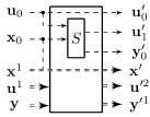
(b)

Figure 15: (a) Unit delay feedback of $S$, (b) $\mathsf{AddDelay}.S$

Finally we can introduce the transformer $\mathsf{DelayFeedback}.init.S$:

Definition 9.

If $init$ is a predicate on the initial value of the feedback variable $u$ and $S$ is a predicate transformer as described above, then unit delay feedback is given by

$$\begin{array}[]{l}\mathsf{DelayFeedback}.init.S=[\mathbf{x}\leadsto\mathbf{u},\mathbf{x},\mathbf{y}\;|\;init.\mathbf{u}_{0}]\;;\,\mathsf{IterateNextOmega}(\mathsf{AddDelay}.S)\;;\,[\mathbf{u},\mathbf{x},\mathbf{y}\leadsto\mathbf{y}]\end{array}$$

The intuition behind the above definition is that if we plug $\mathsf{AddDelay}.S$ (Figure 15b) into Figure 13, using the tuple $(\mathbf{u},\mathbf{x},\mathbf{y})$ instead of $\mathbf{x}$, then we obtain the desired system of Figure 15a.

A major result of this section is that the operators $\mathsf{AddDelay}$ and $\mathsf{DelayFeedback}$ preserve refinement:

Theorem 14.

If $S$ is a predicate transformer as above then

1. $S\sqsubseteq S^{\prime}\Rightarrow\mathsf{AddDelay}.S\sqsubseteq\mathsf{AddDelay}.S^{\prime}$

2. $S\sqsubseteq S^{\prime}\Rightarrow\mathsf{DelayFeedback}.S\sqsubseteq\mathsf{DelayFeedback}.S^{\prime}$

The results presented so far in this section apply to any predicate transformer $S$ with the structure described above (inputs $u,x$ and outputs $v,y$). In practice, we often describe transformers as symbolic transition systems, that is, using a predicate $init$ specifying the set of initial states, a predicate $p$ specifying the set of legal inputs, and a relation $r$ specifying the transition and output relations. If $S$ is obtained from a symbolic transition system, that is, if $S$ has the form $\{u,x\;|\;p.u.x\}\;;\,$ $[u,x\leadsto u^{\prime},y\;|\;r.u.u^{\prime}.x.y]$, then we can prove the following:

Theorem 15.

We have

$$\begin{array}[]{l}\mathsf{DelayFeedback}.init.(\{u,x\,|\,p.u.x\};[u,x\leadsto u^{\prime},y\,|\,r.u.u^{\prime}.x.y])\;=\;\{\mathbf{x}\;|\;\forall\mathbf{u}:init.\mathbf{u}_{0}\Rightarrow(\mathsf{in}.r\mathsf{\,L\,}p).\mathbf{u}.\mathbf{u}^{1}.\mathbf{x}\}\\ \hskip 270.30118pt\;;\,[\mathbf{x}\leadsto\mathbf{y}\;|\;\exists\mathbf{u}:init.\mathbf{u}_{0}\land\Box\,r.\mathbf{u}.\mathbf{u}^{1}.\mathbf{x}.\mathbf{y}]\end{array}$$

This theorem shows that the unit delay feedback of such a predicate transformer is identical to the property transformer semantics of the corresponding symbolic transition system [PT14], which provides a sanity check of our construction. The condition $(\forall\mathbf{u}:init.\mathbf{u}_{0}\Rightarrow(\mathsf{in}.r\mathsf{\,L\,}p).\mathbf{u}.\mathbf{u}^{1}.\mathbf{x})$ is false on input $\mathbf{x}$, if there exists $\mathbf{u}_{0},\ldots,\mathbf{u}_{n}$ and $\mathbf{y}_{0},\ldots,\mathbf{y}_{n-1}$ such that $(\forall i<n:r.\mathbf{u}_{i}.\mathbf{u}_{i+1},\mathbf{x}_{i},\mathbf{y}_{i})$ is true and $p.\mathbf{u}_{n}.\mathbf{x}_{n}$ is false. That is, if with $\mathbf{x}$ it is possible to reach a false assertion, then the system will fail from $\mathbf{x}$, even if non-failing choices are possible.

The intuitive behavior of a system as in Theorem 15 was explained in the beginning of this section. Here we elaborate on this intuition further, explaining in particular how it works for non-deterministic and non-input-receptive systems. The system starts with some initial state $\mathbf{u}_{0}$ and input $\mathbf{x}_{0}$ (the first element of $\mathbf{x}$) and it checks the input condition $p.\mathbf{u}_{0}.\mathbf{x}_{0}$. If the condition is false, then $\mathbf{x}_{0}$ is an illegal input at state $\mathbf{u}_{0}$, and execution fails. Otherwise, the system computes non-deterministically the output $\mathbf{y}_{0}$ and the next state $\mathbf{u}_{1}$, such that $r.\mathbf{u}_{0}.\mathbf{u}_{1}.\mathbf{x}_{0}.\mathbf{y}_{0}$ is true. This ends the first execution step. The system then proceeds with the next step, where it uses $\mathbf{u}_{1}$ and $\mathbf{x}_{1}$ to test again the input condition $p$, and so on. At any point during execution, if $p.\mathbf{u}_{i}.\mathbf{x}_{i}$ becomes false then the system fails. Otherwise the system outputs non-deterministically the infinite sequence $\mathbf{y}_{0},\mathbf{y}_{1},\cdots$. We note that if $r$ is deterministic, i.e., if there exists function $f$ such that $r.u.u^{\prime}.x.y\Leftrightarrow(u^{\prime},y)=f.(u,x)$, then this process yields the standard execution runs.

Example 13.

[Stateful systems in feedback] Consider the following relations modeling systems with state ($u$ and $u^{\prime}$ represent current and next state variables, respectively):

$$R_{1} = [u,x\leadsto u^{\prime},y\;|\;u^{\prime}=u\land y=u]$$ (4)

$$R_{2} = [u,x\leadsto u^{\prime},y\;|\;u^{\prime}=u+1\land y=u]$$ (5)

In $R_{1}$, the next state is equal to the current state. In $R_{2}$, the next state increments the current state by $1$. We will also use the relation $\mathit{StepSum}$ defined in (1). In all three cases the output $y$ is equal to the state. Let $\mathsf{Zero}$ be the predicate given by $\mathsf{Zero}.u=(u=0)$. We compose the above systems by connecting $u^{\prime}$ to $u$ in feedback with unit delay. In all three cases we use the predicate $\mathsf{Zero}$ as $init$, and in all three cases we use input-receptive components, i.e., where $p=\top$. We get:

1. $\mathsf{DelayFeedback}.\mathsf{Zero}.R_{1}=[\mathbf{x}\leadsto\mathbf{y}\,|\,\forall i:\mathbf{y}_{i}=0]$. Since the initial state is $0$, the output is always $0$.

2. $\mathsf{DelayFeedback}.\mathsf{Zero}.R_{2}=[\mathbf{x}\leadsto\mathbf{y}\,|\,\forall i:\mathbf{y}_{i}=i]$. The output at the $i$-th step equals $i$.

3. $\mathsf{DelayFeedback}.\mathsf{Zero}.\mathit{StepSum}=[\mathbf{x}\leadsto sum.\mathbf{x}]$. The output is the summation of the sequence of inputs seen so far.

The three examples above are all input-receptive and deterministic. Our framework can also handle non-input-receptive and non-deterministic systems, as illustrated next:

Example 14 (A deterministic but non-input-receptive system).

Let $R_{3}=\{u,x\;|\;u\leq a\}\;;\,[u,x\leadsto u^{\prime},y\;|\;u^{\prime}=u+x\land y=u]$. $R_{3}$ is similar to $\mathit{StepSum}$, but imposes the condition that at each step the state $u$ is bounded by some constant $a$. Applying feedback we get:

$$\mathsf{DelayFeedback}.\mathsf{Zero}.R_{3}=\{\mathbf{x}|\forall i:sum.\mathbf{x}.i\leq a\}\;;\,[\mathbf{x}\leadsto sum.\mathbf{x}]$$

Note that the local (i.e., at each step) condition $u\leq a$ becomes (after feedback) the global condition that the sum of all elements $\mathbf{x}_{i}$ of every prefix of the input $\mathbf{x}$ must be less or equal to $a$.

Example 15 (A non-deterministic and non-input-receptive system).

We can also weaken the relation $u^{\prime}=u+x\land y=u$ and make the previous system non-deterministic. For example at each step we can choose to compute $u^{\prime}=u+x$ or $u^{\prime}=x$. Let $R_{4}=\{u,x\;|\;u\leq a\}\;;\,[u,x\leadsto u^{\prime},y|(u^{\prime}=u+x\lor u^{\prime}=x)\land y=u]$. Then we get:

$$\begin{array}[]{l}\mathsf{DelayFeedback}.\mathsf{Zero}.R_{4}=\{\mathbf{x}\;|\;\forall i:sum.\mathbf{x}.i\leq a\}\;;\,[\mathbf{x}\leadsto\mathbf{y}\;|\;\mathbf{y}_{0}=0\land(\forall i:\mathbf{y}_{i+1}=\mathbf{y}_{i}+\mathbf{x}_{i}\lor\mathbf{y}_{i+1}=\mathbf{x}_{i})]\end{array}$$

Observe that the global condition on $\mathbf{x}$ remains the same. This is because in the worst case the non-deterministic choice could always pick the alternative $u^{\prime}=u+x$, which leads to higher numbers stored in $u$ compared to the alternative $u^{\prime}=x$.

8 Symbolic Computation

For a relation $R:((A_{1\bot}\times\ldots\times A_{k\bot})\times X)^{\bullet}\to((A_{1\bot}\times\ldots\times A_{k\bot})\times Y)^{\bullet}$, in the $\exists n$ quantifier from the definition of $\mathsf{InstFeedback}.R$, $n$ is bound by $k$. This is so because a strictly increasing sequence $u_{0}<u_{1}<\ldots$ on $A_{1\bot}\times\ldots\times A_{k\bot}$ can have at most $k+1$ elements. Because of this property we have:

$$(\mathsf{fb\_a}.R)^{*}=\bigvee_{i\leq k}(\mathsf{fb\_a}.R)^{i}$$

so we can calculate the feedback symbolically using

$$\mathsf{InstFeedback}.R=\mathsf{fb\_begin}\circ(\bigvee_{i\leq k}(\mathsf{fb\_a}.R)^{i})\circ\mathsf{fb\_b}.R$$

If relation $R$ is defined using a first order formula, then $\mathsf{InstFeedback}.R$ is also a first order formula.

Checking refinement of two relations with $R\sqsubseteq R^{\prime}$ defined by first order formulas is also reduced to checking validity of a first order formula $(\forall x:R.x.\bullet\lor(\forall y:R^{\prime}.x.y\Rightarrow R.x.y)$.

Refinement of predicate transformers of the form $\{p\}\;;\,[r]$ are also reduced to checking validity of a first order formula (Theorem 1). The predicate transformers of the form $\{p\}\;;\,[r]$ are closed to serial and demonic compositions, fusion, and product, so if $p$ and $r$ are defined using first order formulas, then so are the results of these operations (Theorem 1 and 2).

The delay feedback of a predicate transformer of the form $\{p\}\;;\,[r]$ is equivalent by Theorem 15 to a property transformer of the form $\{P\}\;;\,[R]$ where $P$ and $R$ are quantified LTL formulas. Checking the refinement $\mathsf{DelayFeedback}.S\sqsubseteq\mathsf{DelayFeedback}.S^{\prime}$, is reduced by Theorem 14 to checking the refinement $S\sqsubseteq S^{\prime}$ of predicate transformers.

However, $\mathsf{IterateOmega}.F.S$ and $\mathsf{IterateNextOmega}.S$ cannot be reduced always to first order logic or quantified LTL formulas.

9 Implementation in Isabelle

We have stated and proven all results presented in this paper, in the Isabelle/HOL theorem prover. Our theory is built on top of theories for refinement calculus and a semantic formalization of LTL. Proofs omitted from this paper can be found in the Isabelle code, available from http://rcrs.cs.aalto.fi. At the time of this writing our Isabelle theories comprise a total of about 5k lines of code.

Our formalization benefited from the rich collection of Isabelle formalization of mathematical structures used in this paper: partial orders, Boolean algebras, complete lattices, and others.

10 Conclusions

Feedback composition is challenging to define for non-deterministic and non-input-receptive systems, so that refinement is preserved. In this paper we make progress toward this goal. First, we propose an instantaneous feedback composition operator for partial relations with fail and unknown (Section 5). This operator generalizes constructive semantics which are limited to total functions [Mal94, Ber99, EL03]. Second, we propose a feedback-with-unit-delay operator for systems with state (Section 7). Both operators preserve refinement (Theorems 6 and 14).

Our framework can be applied to arbitrary Simulink diagrams by first translating them into predicate transformers that handle current and next state variables as inputs and outputs, respectively, and then applying feedback with unit delay on these variables. Contrary to Simulink, our construction allows instantaneous feedback as well as non-deterministic and non-input-receptive components.

Open problems remain. Seeking a generalization of the feedback operators directly to property transformers, at the semantic level, is a worthwhile albeit difficult goal. With this generalization, we will be able to treat Simulink basic blocks as property transformers, and apply serial and feedback compositions directly.

References

- [AH99] R. Alur and T. Henzinger. Reactive modules. Formal Methods in System Design, 15:7–48, 1999.
- [BB95] R.-J. Back and M. Butler. Exploring summation and product operators in the refinement calculus. In Mathematics of Program Construction, volume 947 of LNCS. Springer, 1995.
- [Ber99] G. Berry. The Constructive Semantics of Pure Esterel, 1999.
- [BS01] M. Broy and K. Stølen. Specification and development of interactive systems: focus on streams, interfaces, and refinement. Springer, 2001.
- [BvW98] R.-J. Back and J. von Wright. Refinement Calculus. A systematic Introduction. Springer, 1998.
- [dA04] L. de Alfaro. Game models for open systems. In Nachum Dershowitz, editor, Verification: Theory and Practice, volume 2772 of Lecture Notes in Computer Science, pages 192–213. Springer, 2004.
- [dAH01] L. de Alfaro and T. Henzinger. Interface automata. In Foundations of Software Engineering (FSE). ACM Press, 2001.
- [DHJP08] L. Doyen, T. Henzinger, B. Jobstmann, and T. Petrov. Interface theories with component reuse. In EMSOFT, pages 79–88, 2008.
- [Dij75] E.W. Dijkstra. Guarded commands, nondeterminacy and formal derivation of programs. Comm. ACM, 18(8):453–457, 1975.
- [DP02] B.A. Davey and H.A. Priestley. Introduction to lattices and order. Cambridge University Press, New York, second edition, 2002.
- [EL03] S. Edwards and E.A. Lee. The semantics and execution of a synchronous block-diagram language. Sci. Comp. Progr., 48:21–42(22), July 2003.
- [FP91] T. Freeman and F. Pfenning. Refinement Types for ML. SIGPLAN Not., 26(6):268–277, May 1991.
- [JDK+14a] X. Jin, J. Deshmukh, J. Kapinski, K. Ueda, and K. Butts. Benchmarks for model transformations and conformance checking. In 1st Intl. Workshop on Applied Verification for Continuous and Hybrid Systems (ARCH), 2014. Benchmark Simulink models available from http://cps-vo.org/group/ARCH/benchmarks.
- [JDK+14b] X. Jin, J. V. Deshmukh, J. Kapinski, K. Ueda, and K. Butts. Powertrain control verification benchmark. In 17th Intl. Conf. on Hybrid Systems: Computation and Control, HSCC ’14, pages 253–262. ACM, 2014.
- [Jon94] B. Jonsson. A fully abstract trace model for dataflow and asynchronous networks. Distrib. Comput., 7(4):197–212, 1994.
- [Kah74] G. Kahn. The semantics of a simple language for parallel programming. In Information Processing 74, Proceedings of IFIP Congress 74. North-Holland, 1974.
- [LT89] N.A. Lynch and M.R. Tuttle. An introduction to input/output automata. CWI Quarterly, 2:219–246, 1989.
- [Mal94] S. Malik. Analysis of cyclic combinational circuits. IEEE Trans. Computer-Aided Design, 13(7):950–956, 1994.
- [Mil90] J. K. Millen. Hookup security for synchronous machines. In Computer Security Foundations Workshop III, pages 84–90, 1990.
- [MTH90] R. Milner, M. Tofte, and R. Harper. The Definition of Standard ML. MIT Press, Cambridge, MA, USA, 1990.
- [NPW02] T. Nipkow, L. C. Paulson, and M. Wenzel. Isabelle/HOL — A Proof Assistant for Higher-Order Logic. LNCS 2283. Springer, 2002.
- [Plo76] G. D. Plotkin. A powerdomain construction. SIAM Journal on Computing, 5(3):452–487, 1976.
- [Pnu77] A. Pnueli. The temporal logic of programs. In FOCS, 1977.
- [Pre14] V. Preoteasa. Formalization of refinement calculus for reactive systems. Archive of Formal Proofs, October 2014. http://afp.sf.net/entries/RefinementReactive.shtml.
- [PT14] V. Preoteasa and S. Tripakis. Refinement calculus of reactive systems. In Embedded Software (EMSOFT). ACM, 2014.
- [RKJ08] P. M. Rondon, M. Kawaguci, and R. Jhala. Liquid types. SIGPLAN Not., 43(6):159–169, 2008.
- [Tar55] A. Tarski. A lattice-theoretical fixpoint theorem and its applications. Pacific J. Math., 5:285–309, 1955.
- [TLHL11] S. Tripakis, B. Lickly, T. A. Henzinger, and E. A. Lee. A Theory of Synchronous Relational Interfaces. ACM Transactions on Programming Languages and Systems (TOPLAS), 33(4), July 2011.
- [TS14] S. Tripakis and C. Shaver. Feedback in Synchronous Relational Interfaces. In From Programs to Systems, volume 8415 of LNCS, pages 249–266. Springer, 2014.
- [XP99] H. Xi and F. Pfenning. Dependent types in practical programming. In POPL, pages 214–227. ACM, 1999.