On solving large-scale limited-memory quasi-Newton equations

Abstract.

We consider the problem of solving linear systems of equations arising with limited-memory members of the restricted Broyden class of updates and the symmetric rank-one (SR1) update. In this paper, we propose a new approach based on a practical implementation of the compact representation for the inverse of these limited-memory matrices. Numerical results suggest that the proposed method compares favorably in speed and accuracy to other algorithms and is competitive with several update-specific methods available to only a few members of the Broyden class of updates. Using the proposed approach has an additional benefit: The condition number of the system matrix can be computed efficiently.

1. Introduction

We consider linear systems of the following form:

(1) $$B_{k+1}r=z,$$

where $r,z\in\Re^{n}$ and $B_{k+1}\in\Re^{n\times n}$ is a limited-memory quasi-Newton matrix obtained from applying $k+1$ Broyden class updates to an initial matrix $B_{0}$. We assume $n$ is large, and thus, explicitly forming and storing $B_{k+1}$ is impractical or impossible; moreover, in this setting, we assume limited-memory quasi-Newton matrices so that only the most recently-computed $k$ updates are stored and used to update $B_{0}$. In practice, the value of $k$ is small, i.e., less than 10 (see e.g.,  [5]), making $k\ll n$. Problems such as (1) arise in quasi-Newton line-search and trust-region methods for large-scale optimization (see, e.g.,  [6, 7, 12, 18]), as well as in preconditioning iterative solvers (see, e.g.,  [16, 19]). In this paper, we propose a compact formulation of $B_{k+1}^{-1}$ that can be used to efficiently solve (1).

Traditional quasi-Newton methods for minimizing a continuously differentiable function $f:\Re^{n}\rightarrow\Re$ generate a sequence of iterates $\{x_{k}\}$ such that $f$ is strictly decreasing on this sequence. Moreover, at each iteration, the most-recently computed iterate $x_{k+1}$ is used to update the quasi-Newton matrix by defining a new quasi-Newton pair $(s_{k},y_{k})$ given by

$$s_{k}\mathop{\,{\scriptstyle\stackrel{{\scriptstyle\triangle}}{{=}}}}\,x_{k+1}-x_{k}\quad\text{and}\quad y_{k}\mathop{\,{\scriptstyle\stackrel{{\scriptstyle\triangle}}{{=}}}}\,\nabla f(x_{k+1})-\nabla f(x_{k}).$$

In the case of the Broyden class updates, $B_{k+1}$ is updated as follows:

(2) $$B_{k+1}=B_{k}-\frac{1}{s_{k}^{T}B_{k}s_{k}}B_{k}s_{k}s_{k}^{T}B_{k}+\frac{1}{y_{k}^{T}s_{k}}y_{k}y_{k}^{T}+\phi(s_{k}^{T}B_{k}s_{k})w_{k}w_{k}^{T},$$

with

$$w_{k}=\frac{y_{k}}{y_{k}^{T}s_{k}}-\frac{B_{k}s_{k}}{s_{k}^{T}B_{k}s_{k}},$$

where $\phi\in\Re$. The most well-known quasi-Newton update is the Broyden-Fletcher-Goldfarb-Shanno (BFGS) update, which is obtained by setting $\phi=0$. While this is the most widely-used update, research has suggested that other values of $\phi$ may lead to faster convergence [20, 4, 14]. Because of this interest in other values of $\phi$, the entire Broyden class (i.e., $\phi\in\Re$) of quasi-Newton methods has been generalized to solve minimization problems over Riemannian manifolds [13]. For these reasons, in this paper, we consider solving (1) for other values of $\phi$ other than $\phi=0$ (the BFGS update). In particular, we consider the restricted Broyden class of updates, where $\phi\in[0,1]$. Under mild assumptions, quasi-Newton matrices in this class are positive definite, a property that is important for computing search directions in optimization. We also consider the special case of the symmetric rank-one (SR1) update, an update that has been of recent interest in trust-region methods for unconstrained optimization [2, 1]. (For more details on limited-memory quasi-Newton matrices and the Broyden class of matrices see, e.g., [5, 12, 18].)

Solving systems of the form (1) can be done efficiently in the case of the BFGS update ($\phi=0$) using the well-known two-loop recursion [17] (see A for details). However, there is no known corresponding recursion method for other updates of the Broyden class (see [18, p.190]); in fact, for this reason many researchers prefer the BFGS update. In this paper we present various methods for solving linear systems of equations with limited-memory quasi-Newton matrices. The main contribution of this paper is a new approach by formulating a compact representation for the inverse of any member of the restricted Broyden class. This representation allows us to efficiently solve linear systems of the form (1). The compact formulation for the inverse of these matrices is based on ideas found in [10], where a compact formulation for the restricted Broyden class of matrices is presented. An additional benefit of our proposed approach is the ability to calculate the eigenvalues of the limited-memory matrix, and hence, the condition number of the linear system.

This paper is organized in seven main sections. In Section 2, we present current methods for solving linear systems with a limited-memory quasi-Newton matrix. In Section 3, we review the compact formulation for matrices obtained using the restricted Broyden class of updates. The compact formulation for the inverse of these matrices is presented in Section 4. In Section 5, we provide a practical implementation for solving systems of the form (1) when the system matrix is either a member of the restricted Broyden class or an SR1 matrix. In addition, we discuss how to compute the condition number of the linear system being solved and how to obtain additional computational savings when a new quasi-Newton pair is computed. We present numerical experiments in Section 6 that demonstrate the competitiveness of our proposed approach. Finally, concluding remarks are in Section 7.

2. Current methods

One approach to solve linear equations with members of the Broyden class is to use the Sherman-Morrison-Woodbury (SMW) formula to update the inverse after each rank-one change (see, e.g.,  [11]). Thus, to compute the inverse after a rank-two update, the SMW formula may be applied twice. (For algorithmic details on this approach, see B.) Alternatively, linear solves with a general member of the Broyden class can be performed using the following recursion formula found in [7] for $H_{k+1}$, the inverse of $B_{k+1}$. Specifically, the inverse of $B_{k+1}$ in (2) is given by the following rank-two update:

(3) $$H_{k+1}=H_{k}+\frac{1}{s_{k}^{T}y_{k}}s_{k}s_{k}^{T}-\frac{1}{y_{k}^{T}H_{k}y_{k}}H_{k}y_{k}y_{k}^{T}H_{k}+\Phi_{k}(y_{k}^{T}H_{k}y_{k})v_{k}v_{k}^{T},$$

where

(4) $$v_{k}=\frac{s_{k}}{y_{k}^{T}s_{k}}-\frac{H_{k}y_{k}}{y_{k}^{T}H_{k}y_{k}},\ \text{and}\ \ \Phi_{k}=\frac{(1-\phi)(y_{k}^{T}s_{k})^{2}}{(1-\phi)(y_{k}^{T}s_{k})^{2}+\phi(y_{k}^{T}H_{k}y_{k})(s_{k}^{T}B_{k}s_{k})},\ \$$

and $H_{k}\mathop{\,{\scriptstyle\stackrel{{\scriptstyle\triangle}}{{=}}}}\,B_{k}^{-1}$. (Algorithmic details associated with this approach can be found in C.)

The method proposed in this paper makes use of the so-called compact formulation of quasi-Newton matrices that not only appears to be competitive in terms of speed but also yields additional information about the system matrix.

3. Compact representation

In this section, we briefly review the compact representation of members of the Broyden class of quasi-Newton matrices.

Given $k+1$ update pairs of the form $\{(s_{i},y_{i})\}$, the compact formulation of $B_{k+1}$ is given by

(5) $$B_{k+1}=B_{0}+\Psi_{k}M_{k}\Psi_{k}^{T},$$

where $M_{k}$ is a square matrix and $B_{0}\in\Re^{n\times n}$ is an initial matrix, which is often taken to be a scalar multiple of the identity. (Note that the size of $\Psi$ is not specified.) The compact formulation of members of the Broyden class of updates are defined in terms of

$$S_{k} = [\ s_{0}\ \ s_{1}\ \ s_{2}\ \ \cdots\ \ s_{k}\ ]\ \in\ \Re^{n\times(k+1)},$$

$$Y_{k} = [\ y_{0}\ \ y_{1}\ \ y_{2}\ \ \cdots\ \ y_{k}\ ]\ \in\ \Re^{n\times(k+1)},$$

and the following decomposition of $S_{k}^{T}Y_{k}\in\Re^{(k+1)\times(k+1)}$:

$$S_{k}^{T}Y_{k}=L_{k}+D_{k}+R_{k},$$

where $L_{k}$ is strictly lower triangular, $D_{k}$ is diagonal, and $R_{k}$ is strictly upper triangular.

Assuming all updates are well defined, Erway and Marcia [10] derive the compact formulation for all members of the Broyden class for $\phi\in[0,1]$. In particular, for any $\phi\in[0,1]$, the compact formulation for $B_{k+1}$ is given by (5) where

(6) $$\Psi_{k}=\begin{bmatrix}B_{0}S_{k}&Y_{k}\end{bmatrix}\quad\text{and}\quad M_{k}\ =\ -\begin{bmatrix}S_{k}^{T}B_{0}S_{k}-\phi\Lambda_{k}&\ \ (L_{k}-\phi\Lambda_{k})\\ (L_{k}-\phi\Lambda_{k})^{T}&-(D_{k}+\phi\Lambda_{k})\end{bmatrix}^{-1},$$

where

(7) $$\Lambda_{k}=\underset{0\leq i\leq k}{\text{diag}}\ (\lambda_{i}),\quad\text{where }\lambda_{i}=\frac{1}{\displaystyle-\frac{1-\phi}{s_{i}^{T}B_{i}s_{i}}-\frac{\phi}{s_{i}^{T}y_{i}}}\ \ \text{for $0\leq i\leq k$.}$$

When $\phi=0$, this representation simplifies to the BFGS compact representation found in [5]. In the limited-memory case, $k\ll n$, and thus, $M_{k}$ is easily inverted.

4. Inverses

In this section, we present the compact formulation for the inverse of any member of the restricted Broyden class of matrices and for SR1 matrices. We then demonstrate how this compact formulation can be used to solve linear systems with these limited-memory matrices. Finally, we discuss computing the condition number of the linear system and potential computational savings when a new quasi-Newton pair is computed.

The main contribution of this paper is formulating a compact representation for the inverse for any member of the restricted Broyden class. It should be noted that the compact formulation for the inverse of a BFGS matrix is already known (see  [5]). We now derive a general expression for the compact representation of any member of the restricted Broyden class. To do this, we apply the Sherman-Morrison-Woodbury formula (see, e.g., [11]) to the compact representation of $B_{k+1}$ found in (5):

$$B_{k+1}^{-1}=B_{0}^{-1}+B_{0}^{-1}\Psi_{k}\left(-M_{k}^{-1}-\Psi_{k}^{T}B_{0}^{-1}\Psi_{k}\right)^{-1}\Psi_{k}^{T}B_{0}^{-1}.$$

For quasi-Newton matrices it is conventional to let $H_{i}$ denote the inverse of $B_{i}$ for each $i$; using this notation, the inverse of $B_{k+1}^{-1}$ is given by

(8) $$H_{k+1}=H_{0}+H_{0}\Psi_{k}\left(-M_{k}^{-1}-\Psi_{k}^{T}H_{0}\Psi_{k}\right)^{-1}\Psi_{k}^{T}H_{0}.$$

Since $H_{0}\Psi_{k}=H_{0}[B_{0}S_{k}\,\,\,Y_{k}]=[S_{k}\,\,\,H_{0}Y_{k}],$ (8) can be written as

(9) $$H_{k+1}=H_{0}+[\ S_{k}\ \ \ H_{0}Y_{k}\ ](-M_{k}^{-1}-\Psi_{k}^{T}H_{0}\Psi_{k})^{-1}\begin{bmatrix}S_{k}^{T}\\ Y_{k}^{T}H_{0}\end{bmatrix}.$$

Finally, (9) can be simplified using

$$\Psi_{k}^{T}H_{0}\Psi_{k}=\begin{bmatrix}S_{k}^{T}B_{0}S_{k}&S_{k}^{T}Y_{k}\\ Y_{k}^{T}S_{k}&Y_{k}^{T}H_{0}Y_{k}\end{bmatrix}$$

to obtain

$$(-M_{k}^{-1}-\Psi_{k}^{T}H_{0}\Psi_{k})^{-1}$$

$$= \left(\begin{bmatrix}S_{k}^{T}B_{0}S_{k}-\phi\Lambda_{k}&\ \ (L_{k}-\phi\Lambda_{k})\\ (L_{k}-\phi\Lambda_{k})^{T}&-(D_{k}+\phi\Lambda_{k})\end{bmatrix}-\begin{bmatrix}S_{k}^{T}B_{0}S_{k}&S_{k}^{T}Y_{k}\\ Y_{k}^{T}S_{k}&Y_{k}^{T}H_{0}Y_{k}\end{bmatrix}\right)^{-1}$$

$$= \begin{bmatrix}-\phi\Lambda_{k}&L_{k}-\phi\Lambda_{k}-S_{k}^{T}Y_{k}\\ L_{k}^{T}-\phi\Lambda_{k}-Y_{k}^{T}S_{k}&-D_{k}-\phi\Lambda_{k}-Y_{k}^{T}H_{0}Y_{k}\end{bmatrix}^{-1}$$

$$= \begin{bmatrix}-\phi\Lambda_{k}&-R_{k}-D_{k}-\phi\Lambda_{k}\\ -R_{k}^{T}-D_{k}-\phi\Lambda_{k}&-D_{k}-\phi\Lambda_{k}-Y_{k}^{T}H_{0}Y_{k}\end{bmatrix}^{-1}.$$

In other words, the compact formulation for the inverse of a member of the restricted Broyden class is given by

(10) $$H_{k+1}=H_{0}+\tilde{\Psi}_{k}\tilde{M}_{k}\tilde{\Psi}_{k}^{T}\quad\text{where}\quad\tilde{\Psi}_{k}\mathop{\,{\scriptstyle\stackrel{{\scriptstyle\triangle}}{{=}}}}\,[S_{k}\,\,\,H_{0}Y_{k}],$$

and

(11) $$\tilde{M}_{k}\mathop{\,{\scriptstyle\stackrel{{\scriptstyle\triangle}}{{=}}}}\,\begin{bmatrix}-\phi\Lambda_{k}&-R_{k}-D_{k}-\phi\Lambda_{k}\\ -R_{k}^{T}-D_{k}-\phi\Lambda_{k}&-D_{k}-\phi\Lambda_{k}-Y_{k}^{T}H_{0}Y_{k}\end{bmatrix}^{-1}.$$

In the following section, we discuss a practical method to compute $\tilde{M}_{k}$. In D, we explore remarkable relationships between various updates.

5. Recursive formulation and practical implementation

In this section, we present a practical method to compute $\tilde{M}_{k}$ in (10) given by (11). We begin by providing an alternative expression for $\tilde{M}_{0}$ that will allow us to define a recursion method to compute $\tilde{M}_{k}$.

Lemma 1. Suppose $H_{1}=H_{0}+\tilde{\Psi}_{0}\tilde{M}_{0}\tilde{\Psi}_{0}^{T}$, is the inverse of a member of the restricted Broyden class of updates after performing one update. Then,

(12) $$\tilde{M}_{0}=\begin{bmatrix}\tilde{\alpha}_{0}&\tilde{\beta}_{0}\\ \tilde{\beta}_{0}&\tilde{\delta}_{0}\end{bmatrix},$$

where

(13) $$\tilde{\alpha}_{0}=\frac{1}{s_{0}^{T}y_{0}}+\Phi_{0}\frac{y_{0}^{T}H_{0}y_{0}}{(s_{0}^{T}y_{0})^{2}},\quad\tilde{\beta}_{0}=-\frac{\Phi_{0}}{y_{0}^{T}s_{0}},\quad\tilde{\delta}_{0}=-\frac{1-\Phi_{0}}{y_{0}^{T}H_{0}y_{0}},$$

and $\Phi_{0}$ is given in (4).

Proof. Expanding (3), yields

$$H_{1} = H_{0}+\left(\frac{1}{s_{0}^{T}y_{0}}+\Phi_{0}\frac{y_{0}^{T}H_{0}y_{0}}{(s_{0}^{T}y_{0})^{2}}\right)s_{0}s_{0}^{T}-\frac{\Phi_{0}}{y_{0}^{T}s_{0}}H_{0}y_{0}s_{0}^{T}$$

$$\qquad-\frac{\Phi_{0}}{y_{0}^{T}s_{0}}s_{0}y_{0}^{T}H_{0}-\frac{1-\Phi_{0}}{y_{0}^{T}H_{0}y_{0}}H_{0}y_{0}y_{0}^{T}H_{0},$$

which simplifies to

(14) $$H_{1}=H_{0}+\begin{bmatrix}s_{0}&H_{0}y_{0}\end{bmatrix}\begin{bmatrix}\tilde{\alpha}_{0}&\tilde{\beta}_{0}\\ \tilde{\beta}_{0}&\tilde{\delta}_{0}\end{bmatrix}\begin{bmatrix}s_{0}^{T}\\ y_{0}^{T}H_{0}\end{bmatrix},$$

where $\tilde{\alpha}_{0}$, $\tilde{\beta}_{0}$, and $\tilde{\delta}_{0}$ are defined as in (13) and $\Phi_{0}$ is given by (4). Note the (14) is of the form $H_{1}=H_{0}+\tilde{\Psi}_{0}\tilde{M}_{0}\tilde{\Psi}_{0}^{T}$.

We now show that $\tilde{M}_{0}$ defined by (12) and (13) is equivalent to (11) with $k=0$. To see this, we simplify the entries of (12). First, define

$$\Delta_{0}\mathop{\,{\scriptstyle\stackrel{{\scriptstyle\triangle}}{{=}}}}\,(1-\phi)(y_{0}^{T}s_{0})^{2}+\phi(y_{0}^{T}H_{0}y_{0})(s_{0}^{T}B_{0}s_{0}).$$

Note that $\Delta_{0}\neq 0$ since $H_{0}$ and $B_{0}$ are positive definite and $\phi\in[0,1]$. Then, $\Phi_{0}=(1-\phi)(s_{0}^{T}y_{0})^{2}/\Delta_{0},$ and thus,

$$\tilde{\alpha}_{0}=\frac{1}{s_{0}^{T}y_{0}}+\frac{(1-\phi)y_{0}^{T}H_{0}y_{0}}{\Delta_{0}},\ \ \tilde{\beta}_{0}=-\frac{(1-\phi)(s_{0}^{T}y_{0})}{\Delta_{0}},\ \ \text{and}\ \ \tilde{\delta}_{0}=-\frac{\phi(s_{0}^{T}B_{0}s_{0})}{\Delta_{0}}.$$

Consider the inverse of (12), which is given by

(15) $$\begin{bmatrix}\tilde{\alpha}_{0}&\tilde{\beta}_{0}\\ \tilde{\beta}_{0}&\tilde{\delta}_{0}\end{bmatrix}^{-1}=\frac{1}{\tilde{\alpha}_{0}\tilde{\delta}_{0}-\tilde{\beta}_{0}^{2}}\begin{bmatrix}\tilde{\delta}_{0}&-\tilde{\beta}_{0}\\ -\tilde{\beta}_{0}&\tilde{\alpha}_{0}\end{bmatrix}.$$

We now simplify the entries on the right side of (15). The determinant of (12) is given by

(16) $$\!\!\!\!\!\!\tilde{\alpha}_{0}\tilde{\delta}_{0}-\tilde{\beta}_{0}^{2}\!=\!\frac{-(1-\Phi_{0})}{(s_{0}^{T}y_{0})(y_{0}^{T}H_{0}y_{0})}-\frac{\Phi_{0}(1-\Phi_{0})}{(s_{0}^{T}y_{0})^{2}}-\frac{\Phi_{0}^{2}}{(s_{0}^{T}y_{0})^{2}}\!=\!\frac{1}{\Delta_{0}}\left(\frac{s_{0}^{T}B_{0}s_{0}}{\lambda_{0}}\right)\!,$$

where $\lambda_{0}$ in (16) is defined in (7). Thus, the first entry of (15) is given by

(17) $$\frac{\tilde{\delta}_{0}}{\tilde{\alpha}_{0}\tilde{\delta}_{0}-\tilde{\beta}_{0}^{2}}=-\frac{\phi(s_{0}^{T}B_{0}s_{0})}{\Delta_{0}}\frac{\Delta_{0}\lambda_{0}}{s_{0}^{T}B_{0}s_{0}}=-\phi\lambda_{0}.$$

The off-diagonal elements of the right-hand side of (15) simplify as follows:

(18) $$\frac{\tilde{\beta}_{0}}{\tilde{\alpha}_{0}\tilde{\delta}_{0}-\tilde{\beta}_{0}^{2}}=-\left(\frac{(1-\phi)(s_{0}^{T}y_{0})}{\Delta_{0}}\right)\left({\Delta_{0}}\left(\frac{\lambda_{0}}{s_{0}^{T}B_{0}s_{0}}\right)\right)=s_{0}^{T}y_{0}+\phi\lambda_{0}.$$

Finally, the last entry of (15) can be simplified as follows:

(19) $$\frac{\tilde{\alpha}_{0}}{\tilde{\alpha}_{0}\tilde{\delta}_{0}-\tilde{\beta}_{0}^{2}} = \frac{1}{s_{0}^{T}y_{0}}\frac{\Delta_{0}\lambda_{0}}{s_{0}^{T}B_{0}s_{0}}+(1-\phi)y_{0}^{T}H_{0}y_{0}\frac{\lambda_{0}}{s_{0}^{T}B_{0}s_{0}}$$

$$= -s_{0}^{T}y_{0}-\phi\lambda_{0}-y_{0}^{T}H_{0}y_{0}.$$

(For details in the calculations of (16), (18), (19), see F.) Thus, (15) together with (17), (18), and (19) gives

$$\begin{bmatrix}\tilde{\alpha}_{0}&\tilde{\beta}_{0}\\ \tilde{\beta}_{0}&\tilde{\delta}_{0}\end{bmatrix}^{-1}=\begin{bmatrix}-\phi\lambda_{0}&-s_{0}^{T}y_{0}-\phi\lambda_{0}\\ -s_{0}^{T}y_{0}-\phi\lambda_{0}&-s_{0}^{T}y_{0}-\phi\lambda_{0}-y_{0}^{T}H_{0}y_{0}\end{bmatrix},$$

showing that $\tilde{M}_{0}$ defined by (12) and (13) is equivalent to (11) with $k=0$. $\square$

Together with Lemma 1, the following theorem shows how $\tilde{M}_{k}$ is related to $\tilde{M}_{k-1}$; from this, we present an algorithm to compute $\tilde{M}_{k}$ using recursion. This computation avoids explicitly forming $B_{k}$, which is used in the definition of $\Lambda_{k}$ and $\Phi_{k}$.

Theorem 1. Suppose $H_{j+1}=H_{0}+\tilde{\Psi}_{j}\tilde{M}_{j}\tilde{\Psi}_{j}^{T}$ as in (10) for all $j\in\{0,\dots,k\}$, is the inverse of a member of the Broyden class of updates for a fixed $\phi\in[0,1]$. If $\tilde{M}_{0}$ is defined by (12), then for all $j\in\{1,\ldots k\}$, $\tilde{M}_{j}$ satisfies the recursion relation

(20) $$\tilde{M}_{j}=\Pi_{j}^{T}\!\!\begin{bmatrix}\tilde{M}_{j-1}+\tilde{\delta}_{j}\tilde{u}_{j}\tilde{u}_{j}^{T}&\tilde{\beta}_{j}\tilde{u}_{j}&\tilde{\delta}_{j}\tilde{u}_{j}\\ \tilde{\beta}_{j}\tilde{u}_{j}^{T}&\tilde{\alpha}_{j}&\tilde{\beta}_{j}\\ \tilde{\delta}_{j}\tilde{u}_{j}^{T}&\tilde{\beta}_{j}&\tilde{\delta}_{j}\end{bmatrix}\!\Pi_{j},\ \text{where}\ \Pi_{j}\!=\!\!\begin{bmatrix}I_{j}&0&0&0\\ 0&0&1&0\\ 0&I_{j}&0&0\\ 0&0&0&1\end{bmatrix}$$

is such that $\begin{bmatrix}\tilde{\Psi}_{j-1}&s_{j}&H_{0}y_{j}\end{bmatrix}\Pi_{j}=\tilde{\Psi}_{j},$ and

$$\tilde{\alpha}_{j}=\frac{1}{s_{j}^{T}y_{j}}+\Phi_{j}\frac{y_{j}^{T}H_{j}y_{j}}{(s_{j}^{T}y_{j})^{2}},\quad\tilde{\beta}_{j}=-\frac{\Phi_{j}}{y_{j}^{T}s_{j}},\quad\tilde{\delta}_{j}=-\frac{1-\Phi_{j}}{y_{j}^{T}H_{j}y_{j}},$$

and $\tilde{u}_{j}=\tilde{M}_{j-1}\tilde{\Psi}_{j-1}^{T}y_{j}$.

Proof. This proof is by induction on $j$. For the base case, we show that equation (20) holds for $j=1$. Setting $k=1$ in (3) yields

(21) $$H_{2}=H_{1}+\begin{bmatrix}s_{1}&H_{1}y_{1}\end{bmatrix}\begin{bmatrix}\tilde{\alpha}_{1}&\tilde{\beta}_{1}\\ \tilde{\beta}_{1}&\tilde{\delta}_{1}\end{bmatrix}\begin{bmatrix}s_{1}^{T}\\ y_{1}^{T}H_{1}\end{bmatrix},$$

where

$$\tilde{\alpha}_{1}=\frac{1}{s_{1}^{T}y_{1}}+\Phi_{1}\frac{y_{1}^{T}H_{1}y_{1}}{(s_{1}^{T}y_{1})^{2}},\quad\tilde{\beta}_{1}=-\frac{\Phi_{1}}{y_{1}^{T}s_{1}},\quad\text{and}\quad\tilde{\delta}_{1}=-\frac{1-\Phi_{1}}{y_{1}^{T}H_{1}y_{1}}.$$

By Lemma 1, (21) can be written as

(22) $$H_{2}=H_{0}+\tilde{\Psi}_{0}\tilde{M}_{0}\tilde{\Psi}_{0}^{T}+\begin{bmatrix}s_{1}&H_{1}y_{1}\end{bmatrix}\begin{bmatrix}\tilde{\alpha}_{1}&\tilde{\beta}_{1}\\ \tilde{\beta}_{1}&\tilde{\delta}_{1}\end{bmatrix}\begin{bmatrix}s_{1}^{T}\\ y_{1}^{T}H_{1}\end{bmatrix},$$

where $\tilde{\Psi}_{0}=[S_{0}\,\,\,H_{0}Y_{0}]$ and $\tilde{M}_{0}$ is given by (12). Letting $\tilde{u}_{1}=\tilde{M}_{0}\tilde{\Psi}_{0}^{T}y_{1}$, we have that

(23) $$H_{1}y_{1}=\left(H_{0}+\tilde{\Psi}_{0}\tilde{M}_{0}\tilde{\Psi}_{0}^{T}\right)y_{1}=H_{0}y_{1}+\tilde{\Psi}_{0}\tilde{u}_{1}.$$

Substituting (23) into the last quantity on the right side of (22) yields

$$\begin{bmatrix}s_{1}&H_{1}y_{1}\end{bmatrix}\begin{bmatrix}\tilde{\alpha}_{1}&\tilde{\beta}_{1}\\ \tilde{\beta}_{1}&\tilde{\delta}_{1}\end{bmatrix}\begin{bmatrix}s_{1}^{T}\\ y_{1}^{T}H_{1}\end{bmatrix} = \begin{bmatrix}s_{1}&H_{0}y_{1}+\tilde{\Psi}_{0}\tilde{u}_{1}\end{bmatrix}\begin{bmatrix}\tilde{\alpha}_{1}&\tilde{\beta}_{1}\\ \tilde{\beta}_{1}&\tilde{\delta}_{1}\end{bmatrix}\begin{bmatrix}s_{1}^{T}\\ y_{1}^{T}H_{0}+\tilde{u}_{1}^{T}\tilde{\Psi}_{0}^{T}\end{bmatrix}$$

$$= \begin{bmatrix}\tilde{\Psi}_{0}&s_{1}&H_{0}y_{1}\end{bmatrix}\begin{bmatrix}\tilde{\delta}_{1}\tilde{u}_{1}\tilde{u}_{1}^{T}&\tilde{\beta}_{1}\tilde{u}_{1}&\tilde{\delta}_{1}\tilde{u}_{1}\\ \tilde{\beta}_{1}\tilde{u}_{1}^{T}&\tilde{\alpha}_{1}&\tilde{\beta}_{1}\\ \tilde{\delta}_{1}\tilde{u}_{1}^{T}&\tilde{\beta}_{1}&\tilde{\delta}_{1}\end{bmatrix}\begin{bmatrix}\tilde{\Psi}_{0}^{T}\\ s_{1}^{T}\\ y_{1}^{T}H_{0}\end{bmatrix}.$$

Letting $\Pi_{1}$ be defined as in (20) with $j=1$, gives that $\begin{bmatrix}\tilde{\Psi}_{0}&s_{1}&H_{0}y_{1}\end{bmatrix}\Pi_{1}=\tilde{\Psi}_{1},$ and thus,

$$H_{2}=H_{0}+\tilde{\Psi}_{1}\Pi_{1}^{T}\bar{M}_{1}\Pi_{1}\tilde{\Psi}_{1}^{T},$$

where

$$\bar{M}_{1}\mathop{\,{\scriptstyle\stackrel{{\scriptstyle\triangle}}{{=}}}}\,\begin{bmatrix}\tilde{M}_{0}+\tilde{\delta}_{1}\tilde{u}_{1}\tilde{u}_{1}^{T}&\tilde{\beta}_{1}\tilde{u}_{1}&\tilde{\delta}_{1}\tilde{u}_{1}\\ \tilde{\beta}_{1}\tilde{u}_{1}^{T}&\tilde{\alpha}_{1}&\tilde{\beta}_{1}\\ \tilde{\delta}_{1}\tilde{u}_{1}^{T}&\tilde{\beta}_{1}&\tilde{\delta}_{1}\end{bmatrix}.$$

It remains to show that $\tilde{M}_{1}=\Pi_{1}^{T}\bar{M}_{1}\Pi_{1}$; however, for simplicity, we instead show $\tilde{M}_{1}^{-1}=\Pi_{1}^{T}\bar{M}_{1}^{-1}\Pi$.

Notice that $\bar{M}_{1}$ can be written as the product of three matrices:

$$\bar{M}_{1} = \begin{bmatrix}I_{2}&0&\tilde{u}_{1}\\ 0&1&0\\ 0&0&1\end{bmatrix}\begin{bmatrix}\tilde{M}_{0}&0\\ 0&\tilde{N}_{0}\end{bmatrix}\begin{bmatrix}I_{2}&0&0\\ 0&1&0\\ \tilde{u}_{1}^{T}&0&1\end{bmatrix},\ \text{where }\tilde{N}_{0}=\begin{bmatrix}\tilde{\alpha}_{1}&\tilde{\beta}_{1}\\ \tilde{\beta}_{1}&\tilde{\delta}_{1}\end{bmatrix}.$$

Then, $\bar{M}_{1}^{-1}$ is given by

(24) $$\bar{M}_{1}^{-1} = \begin{bmatrix}I&0&0\\ 0&1&0\\ -\tilde{u}_{1}^{T}&0&1\end{bmatrix}\begin{bmatrix}\tilde{M}_{0}^{-1}&0\\ 0&\tilde{N}_{0}^{-1}\end{bmatrix}\begin{bmatrix}I&0&-\tilde{u}_{1}\\ 0&1&0\\ 0&0&1\end{bmatrix}.$$

It can be shown, using similar computations as in the proof of Lemma 1, that

$$\tilde{N}_{0}^{-1} = \frac{1}{\tilde{\alpha}_{1}\tilde{\delta}_{1}-\tilde{\beta}_{1}^{2}}\begin{bmatrix}\tilde{\delta}_{1}&-\tilde{\beta}_{1}\\ -\tilde{\beta}_{1}&\tilde{\alpha}_{1}\end{bmatrix}=\begin{bmatrix}-\phi\lambda_{1}&-s_{1}^{T}y_{1}-\phi\lambda_{1}\\ -s_{1}^{T}y_{1}-\phi\lambda_{1}&-s_{1}^{T}y_{1}-\phi\lambda_{1}-y_{1}^{T}H_{1}y_{1}\end{bmatrix}.$$

Substituting $\tilde{N}_{0}^{-1}$ into (24) and simplifying yields

(25) $$\bar{M}_{1}^{-1}=\begin{bmatrix}\tilde{M}_{0}^{-1}&0&-\tilde{\Psi}_{0}^{T}y_{1}\\ 0&-\phi\lambda_{1}&-s_{1}^{T}y_{1}-\phi\lambda_{1}\\ -y_{1}^{T}\tilde{\Psi}_{0}&-s_{1}^{T}y_{1}-\phi\lambda_{1}&\tilde{u}_{1}^{T}M_{0}^{-1}\tilde{u}_{1}-s_{1}^{T}y_{1}-\phi\lambda_{1}-y_{1}^{T}H_{1}y_{1}\end{bmatrix}.$$

Terms in the (3,3)-entry in the right side of (25) can be simplified using that $\tilde{M}_{0}^{-1}\tilde{u}_{1}=\tilde{\Psi}_{0}^{T}y_{1}$ and that $y_{1}^{T}H_{1}y_{1}=y_{1}^{T}H_{0}y_{1}+y_{1}^{T}\tilde{\Psi}_{0}\tilde{M}_{0}\tilde{\Psi}_{0}^{T}y_{1}$ as follows:

$$\tilde{u}_{1}^{T}\tilde{M}_{0}^{-1}\tilde{u}_{1}-y_{1}^{T}H_{1}y_{1} = y_{1}^{T}\tilde{\Psi}_{0}\tilde{M}_{0}\tilde{\Psi}_{0}^{T}y_{1}-y_{1}^{T}H_{1}y_{1}$$

$$= -y_{1}^{T}H_{0}y_{1}+y_{1}^{T}H_{1}y_{1}-y_{1}^{T}H_{1}y_{1}$$

$$= -y_{1}^{T}H_{0}y_{1}.$$

Thus,

(26) $$\bar{M}_{1}^{-1}=\begin{bmatrix}\tilde{M}_{0}^{-1}&0&-\tilde{\Psi}_{0}^{T}y_{1}\\ 0&-\phi\lambda_{1}&-s_{1}^{T}y_{1}-\phi\lambda_{1}\\ -y_{1}^{T}\tilde{\Psi}_{0}&-s_{1}^{T}y_{1}-\phi\lambda_{1}&-s_{1}^{T}y_{1}-\phi\lambda_{1}-y_{1}^{T}H_{0}y_{1}\end{bmatrix}.$$

Lemma 1, together with the substitution $\tilde{\Psi}_{0}^{T}y_{1}=\displaystyle\begin{pmatrix}S_{0}^{T}y_{1}\\ Y_{0}^{T}H_{0}y_{1}\end{pmatrix}$, gives that

−s0Ty0−ϕλ00−s0Ty0−ϕλ0−y0TH0y0−Y0TH0y1−y1TS0−s1Ty1−ϕλ1−y1TH0Y0−s1Ty1−ϕλ1−y1TH0y1]delimited-[]fragments fragments fragmentss0𝑇y0ϕλ00fragmentss0𝑇y0ϕλ0y0𝑇H0y0fragmentsY0𝑇H0y1fragmentsy1𝑇S0fragmentss1𝑇y1ϕλ1fragmentsy1𝑇H0Y0fragmentss1𝑇y1ϕλ1y1𝑇H0y1\displaystyle\tiny\left[\begin{tabular}[]{cc|ccccc}$-\phi\lambda_{0}$&$0$&$-s_{0}^{T}y_{0}-\phi\lambda_{0}$&$-S_{0}^{T}y_{1}$\\ $0$&$-\phi\lambda_{1}$&$0$&$-s_{1}^{T}y_{1}-\phi\lambda_{1}$\\ \hline\cr$-s_{0}^{T}y_{0}-\phi\lambda_{0}$&$0$&$-s_{0}^{T}y_{0}-\phi\lambda_{0}-y_{0}^{T}H_{0}y_{0}$&$-Y_{0}^{T}H_{0}y_{1}$\\ $-y_{1}^{T}S_{0}$&$-s_{1}^{T}y_{1}-\phi\lambda_{1}$&$-y_{1}^{T}H_{0}Y_{0}$&$-s_{1}^{T}y_{1}-\phi\lambda_{1}-y_{1}^{T}H_{0}y_{1}$\end{tabular}\right] −R0T−D0−ϕΛ00−D0−ϕΛ1−Y0TH0Y0−Y0TH0y1−y1TS0−s1Ty1−ϕλ1−y1TH0Y0−s1Ty1−ϕλ1−y1TH0y1]delimited-[]fragments fragments fragmentsR0𝑇D0ϕΛ00fragmentsD0ϕΛ1Y0𝑇H0Y0fragmentsY0𝑇H0y1fragmentsy1𝑇S0fragmentss1𝑇y1ϕλ1fragmentsy1𝑇H0Y0fragmentss1𝑇y1ϕλ1y1𝑇H0y1\displaystyle\tiny\left[\begin{tabular}[]{cc|ccccc}$-\phi\Lambda_{0}$&$0$&$-R_{0}-D_{0}-\phi\Lambda_{0}$&$-S_{0}^{T}y_{1}$\\ $0$&$-\phi\lambda_{1}$&$0$&$-s_{1}^{T}y_{1}-\phi\lambda_{1}$\\ \hline\cr$-R_{0}^{T}-D_{0}-\phi\Lambda_{0}$&$0$&$-D_{0}-\phi\Lambda_{1}-Y_{0}^{T}H_{0}Y_{0}$&$-Y_{0}^{T}H_{0}y_{1}$\\ $-y_{1}^{T}S_{0}$&$-s_{1}^{T}y_{1}-\phi\lambda_{1}$&$-y_{1}^{T}H_{0}Y_{0}$&$-s_{1}^{T}y_{1}-\phi\lambda_{1}-y_{1}^{T}H_{0}y_{1}$\end{tabular}\right]

$$\Pi_{1}^{T}\bar{M}_{1}^{-1}\Pi_{1}$$

$$= \Pi_{j}^{T}\begin{bmatrix}\tilde{M}_{0}^{-1}&0&-\tilde{\Psi}_{0}^{T}y_{1}\\ 0&-\phi\lambda_{1}&-s_{1}^{T}y_{1}-\phi\lambda_{1}\\ -y_{1}^{T}\tilde{\Psi}_{0}&-s_{1}^{T}y_{1}-\phi\lambda_{1}&-s_{1}^{T}y_{1}-\phi\lambda_{1}-y_{1}^{T}H_{0}y_{1}\end{bmatrix}\Pi_{j}$$

$$= \tiny\left[\begin{tabular}[]{cc|ccccc}$-\phi\lambda_{0}$&$0$&$-s_{0}^{T}y_{0}-\phi\lambda_{0}$&$-S_{0}^{T}y_{1}$\\ $0$&$-\phi\lambda_{1}$&$0$&$-s_{1}^{T}y_{1}-\phi\lambda_{1}$\\ \hline\cr$-s_{0}^{T}y_{0}-\phi\lambda_{0}$&$0$&$-s_{0}^{T}y_{0}-\phi\lambda_{0}-y_{0}^{T}H_{0}y_{0}$&$-Y_{0}^{T}H_{0}y_{1}$\\ $-y_{1}^{T}S_{0}$&$-s_{1}^{T}y_{1}-\phi\lambda_{1}$&$-y_{1}^{T}H_{0}Y_{0}$&$-s_{1}^{T}y_{1}-\phi\lambda_{1}-y_{1}^{T}H_{0}y_{1}$\end{tabular}\right]$$ -ϕλ00--s0Ty0ϕλ0-S0Ty10-ϕλ10--s1Ty1ϕλ1-ϕλ00--s0Ty0ϕλ0-S0Ty10-ϕλ10--s1Ty1ϕλ1

$$= \tiny\left[\begin{tabular}[]{cc|ccccc}$-\phi\Lambda_{0}$&$0$&$-R_{0}-D_{0}-\phi\Lambda_{0}$&$-S_{0}^{T}y_{1}$\\ $0$&$-\phi\lambda_{1}$&$0$&$-s_{1}^{T}y_{1}-\phi\lambda_{1}$\\ \hline\cr$-R_{0}^{T}-D_{0}-\phi\Lambda_{0}$&$0$&$-D_{0}-\phi\Lambda_{1}-Y_{0}^{T}H_{0}Y_{0}$&$-Y_{0}^{T}H_{0}y_{1}$\\ $-y_{1}^{T}S_{0}$&$-s_{1}^{T}y_{1}-\phi\lambda_{1}$&$-y_{1}^{T}H_{0}Y_{0}$&$-s_{1}^{T}y_{1}-\phi\lambda_{1}-y_{1}^{T}H_{0}y_{1}$\end{tabular}\right]$$ -ϕΛ00--R0D0ϕΛ0-S0Ty10-ϕλ10--s1Ty1ϕλ1-ϕΛ00--R0D0ϕΛ0-S0Ty10-ϕλ10--s1Ty1ϕλ1

$$= \begin{bmatrix}-\phi\Lambda_{1}&-R_{1}-D_{1}-\phi\Lambda_{1}\\ -R_{1}^{T}-D_{1}-\phi\Lambda_{1}&-D_{1}-\phi\Lambda_{1}-Y_{1}^{T}H_{0}Y_{1}\end{bmatrix}$$

$$= \tilde{M}_{1}^{-1},$$

proving the base case.

The inductive step is similar to the base case. For the inductive step, we assume the theorem holds for $k=1,\ldots j-1$ and now show it holds for $k=j$. We begin, as before, setting $k=j$ in (3) to obtain

(29) $$H_{j+1}=H_{j}+\begin{bmatrix}s_{j}&H_{j}y_{j}\end{bmatrix}\begin{bmatrix}\tilde{\alpha}_{j}&\tilde{\beta}_{j}\\ \tilde{\beta}_{j}&\tilde{\delta}_{j}\end{bmatrix}\begin{bmatrix}s_{j}^{T}\\ y_{j}^{T}H_{j}\end{bmatrix},$$

where

$$\tilde{\alpha}_{j}=\frac{1}{s_{j}^{T}y_{j}}+\Phi_{j}\frac{y_{j}^{T}H_{j}y_{j}}{(s_{j}^{T}y_{j})^{2}},\quad\tilde{\beta}_{j}=-\frac{\Phi_{j}}{y_{j}^{T}s_{j}},\quad\text{and}\quad\tilde{\delta}_{j}=-\frac{1-\Phi_{j}}{y_{j}^{T}H_{j}y_{j}},$$

Using the induction hypothesis, (29) becomes

$$H_{j+1}=H_{0}+\tilde{\Psi}_{j-1}\tilde{M}_{j-1}\tilde{\Psi}_{j-1}+\begin{bmatrix}s_{j}&H_{j}y_{j}\end{bmatrix}\begin{bmatrix}\tilde{\alpha}_{j}&\tilde{\beta}_{j}\\ \tilde{\beta}_{j}&\tilde{\delta}_{j}\end{bmatrix}\begin{bmatrix}s_{j}^{T}\\ y_{j}^{T}H_{j}\end{bmatrix}.$$

Similar to the base case,

$$\begin{bmatrix}s_{j}&H_{j}y_{j}\end{bmatrix}\begin{bmatrix}\tilde{\alpha}_{j}&\tilde{\beta}_{j}\\ \tilde{\beta}_{j}&\tilde{\delta}_{j}\end{bmatrix}\begin{bmatrix}s_{j}^{T}\\ y_{j}^{T}H_{j}\end{bmatrix}$$

$$= \begin{bmatrix}s_{j}&H_{0}y_{j}+\tilde{\Psi}_{j-1}\tilde{u}_{j}\end{bmatrix}\begin{bmatrix}\tilde{\alpha}_{j}&\tilde{\beta}_{j}\\ \tilde{\beta}_{j}&\tilde{\delta}_{j}\end{bmatrix}\begin{bmatrix}s_{j}^{T}\\ y_{j}^{T}H_{0}+\tilde{u}_{j}^{T}\tilde{\Psi}_{j-1}^{T}\end{bmatrix}$$

$$= \begin{bmatrix}\tilde{\Psi}_{j-1}&s_{j}&H_{0}y_{j}\end{bmatrix}\begin{bmatrix}\tilde{\delta}_{j}\tilde{u}_{j}\tilde{u}_{j}^{T}&\tilde{\beta}_{j}\tilde{u}_{j}&\tilde{\delta}_{j}\tilde{u}_{j}\\ \tilde{\beta}_{j}\tilde{u}_{j}^{T}&\tilde{\alpha}_{j}&\tilde{\beta}_{j}\\ \tilde{\delta}_{j}\tilde{u}_{j}^{T}&\tilde{\beta}_{j}&\tilde{\delta}_{j}\end{bmatrix}\begin{bmatrix}\tilde{\Psi}_{j-1}^{T}\\ s_{j}^{T}\\ y_{j}^{T}H_{0}\end{bmatrix},$$

where $\tilde{u}_{j}=\tilde{M}_{j-1}\tilde{\Phi}^{T}_{j-1}y_{j}$. With $\Pi_{j}$ defined as in (20), then $\begin{bmatrix}\tilde{\Psi}_{j-1}&s_{j}&H_{0}y_{j}\end{bmatrix}\Pi_{j}=\tilde{\Psi}_{j},$ and so $H_{j}=H_{0}+\tilde{\Psi}_{j}\Pi_{j}^{T}\bar{M}_{j}\Pi_{j}\tilde{\Psi}_{j}^{T},$ where

(30) $$\bar{M}_{j}\mathop{\,{\scriptstyle\stackrel{{\scriptstyle\triangle}}{{=}}}}\,\begin{bmatrix}\tilde{M}_{j-1}+\tilde{\delta}_{j}\tilde{u}_{j}\tilde{u}_{j}^{T}&\tilde{\beta}_{j}\tilde{u}_{j}&\tilde{\delta}_{j}\tilde{u}_{j}\\ \tilde{\beta}_{j}\tilde{u}_{j}^{T}&\tilde{\alpha}_{j}&\tilde{\beta}_{j}\\ \tilde{\delta}_{j}\tilde{u}_{j}^{T}&\tilde{\beta}_{j}&\tilde{\delta}_{j}\end{bmatrix}.$$

It remains to show that $\tilde{M}_{j}=\Pi_{j}^{T}\bar{M}_{j}\Pi_{j}$; however, for simplicity, we instead show $\tilde{M}_{j}^{-1}=\Pi_{j}^{T}\bar{M}_{j}^{-1}\Pi_{j}$ using a similar argument as in the base case. In particular, similar to (25), it can be shown that

$$\bar{M}_{j}^{-1}=\begin{bmatrix}\tilde{M}_{j-1}^{-1}&0&-\tilde{\Psi}_{j-1}^{T}y_{j}\\ 0&-\phi\lambda_{j}&-s_{j}^{T}y_{j}-\phi\lambda_{j}\\ -y_{j}^{T}\tilde{\Psi}_{j-1}&-s_{j}^{T}y_{j}-\phi\lambda_{j}&-s_{j}^{T}y_{j}-\phi\lambda_{j}-y_{j}^{T}H_{0}y_{j}\end{bmatrix}.$$

By the inductive hypothesis that (11) holds for $k=j-1$,

$$\tilde{M}_{j-1}^{-1}=\begin{bmatrix}-\phi\Lambda_{j-1}&-R_{j-1}-D_{j-1}-\phi\Lambda_{j-1}\\ -R_{j-1}^{T}-D_{j-1}-\phi\Lambda_{j-1}&-D_{j-1}-\phi\Lambda_{k}-Y_{j-1}^{T}H_{0}Y_{j-1}\end{bmatrix}$$

and so,

−Rj−1T−Dj−1−ϕΛj−10−Dj−1−ϕΛj−1−Yj−1TH0Yj−1−Yj−1TH0yj−yjTSj−1−sjTyj−ϕλj−yjTH0Yj−1−sjTyj−ϕλj−yjTH0yj]delimited-[]fragments fragments fragmentsR𝑗1𝑇D𝑗1ϕΛ𝑗10fragmentsD𝑗1ϕΛ𝑗1Y𝑗1𝑇H0Y𝑗1fragmentsY𝑗1𝑇H0y𝑗fragmentsy𝑗𝑇S𝑗1fragmentss𝑗𝑇y𝑗ϕλ𝑗fragmentsy𝑗𝑇H0Y𝑗1fragmentss𝑗𝑇y𝑗ϕλ𝑗y𝑗𝑇H0y𝑗\displaystyle\tiny\left[\begin{tabular}[]{cc|ccccc}$-\phi\Lambda_{j-1}$&$0$&$-R_{j-1}-D_{j-1}-\phi\Lambda_{j-1}$&$-S_{j-1}^{T}y_{j}$\\ $0$&$-\phi\lambda_{j}$&$0$&$-s_{j}^{T}y_{j}\!-\!\phi\lambda_{j}$\\ \hline\cr$-R_{j-1}^{T}\!\!-\!D_{j-1}\!\!-\!\phi\Lambda_{j-1}$&$0$&$-D_{j-1}\!\!-\!\phi\Lambda_{j-1}\!\!-\!Y_{j-1}^{T}H_{0}Y_{j-1}$&$-Y_{j-1}^{T}H_{0}y_{j}$\\ $-y_{j}^{T}S_{j-1}$&$-s_{j}^{T}y_{j}\!-\!\phi\lambda_{j}$&$-y_{j}^{T}H_{0}Y_{j-1}$&$-s_{j}^{T}y_{j}\!-\!\phi\lambda_{j}\!-\!y_{j}^{T}H_{0}y_{j}$\end{tabular}\right]

$$\Pi_{j}^{T}\bar{M}_{j}^{-1}\Pi_{j}$$

$$= \Pi_{j}^{T}\begin{bmatrix}\tilde{M}_{j-1}^{-1}&0&-\tilde{\Psi}_{j-1}^{T}y_{j}\\ 0&-\phi\lambda_{j}&-s_{j}^{T}y_{j}-\phi\lambda_{j}\\ -y_{j}^{T}\tilde{\Psi}_{j-1}&-s_{j}^{T}y_{j}-\phi\lambda_{j}&-s_{j}^{T}y_{j}-\phi\lambda_{j}-y_{j}^{T}H_{0}y_{j}\end{bmatrix}\Pi_{j}$$

$$= \tiny\left[\begin{tabular}[]{cc|ccccc}$-\phi\Lambda_{j-1}$&$0$&$-R_{j-1}-D_{j-1}-\phi\Lambda_{j-1}$&$-S_{j-1}^{T}y_{j}$\\ $0$&$-\phi\lambda_{j}$&$0$&$-s_{j}^{T}y_{j}\!-\!\phi\lambda_{j}$\\ \hline\cr$-R_{j-1}^{T}\!\!-\!D_{j-1}\!\!-\!\phi\Lambda_{j-1}$&$0$&$-D_{j-1}\!\!-\!\phi\Lambda_{j-1}\!\!-\!Y_{j-1}^{T}H_{0}Y_{j-1}$&$-Y_{j-1}^{T}H_{0}y_{j}$\\ $-y_{j}^{T}S_{j-1}$&$-s_{j}^{T}y_{j}\!-\!\phi\lambda_{j}$&$-y_{j}^{T}H_{0}Y_{j-1}$&$-s_{j}^{T}y_{j}\!-\!\phi\lambda_{j}\!-\!y_{j}^{T}H_{0}y_{j}$\end{tabular}\right]$$ -ϕΛ-j10--R-j1D-j1ϕΛ-j1-S-j1Tyj0-ϕλj0--sjTyjϕλj-ϕΛ-j10--R-j1D-j1ϕΛ-j1-S-j1Tyj0-ϕλj0--sjTyjϕλj

$$= \begin{bmatrix}-\phi\Lambda_{j}&-R_{j}-D_{j}-\phi\Lambda_{j}\\ -R_{j}^{T}-D_{j}-\phi\Lambda_{j}&-D_{j}-\phi\Lambda_{j}-Y_{j}^{T}H_{0}Y_{j}\end{bmatrix}$$

$$= \tilde{M}_{j}^{-1},$$

proving the induction step. $\square$

Using Theorem 1, Algorithm 1 computes $\tilde{M}_{k}$ and then uses the compact formulation for the inverse to solve linear systems of the form (1). There are two parts to the for loop in Algorithm 1: The first half of the loop is used to build products of the form $s_{j}^{T}B_{j}s_{j}$; the second half of the loop computes $\tilde{M}_{k}$, making use of $s_{j}^{T}B_{j}s_{j}$ to compute $\Phi_{j}$. In the special case when $\phi=0$ or $\phi=1$, $\Phi_{j}$ can be quickly computed as $\Phi_{j}=1$ and $\Phi_{j}=0$, respectively.

Define $\phi$, $B_{0}$, and $H_{0}$;

Form $M_{0}$ using (6) and $\tilde{M}_{0}$ using (12);

Let $\Psi_{0}=(B_{0}s_{0}\,\,y_{0})$ and $\tilde{\Psi}_{0}=(s_{0}\,\,H_{0}y_{0})$;

for  $j=1:k$

     

     $\%$ Part 1: Compute $s_{j}^{T}B_{j}s_{j}$

     $u_{j}\leftarrow M_{j-1}(\Psi_{j-1}^{T}s_{j}$);

     $s_{j}^{T}B_{j}s_{j}\leftarrow s_{j}^{T}B_{0}s_{j}+(s_{j}^{T}\Psi_{j-1})u_{j}$;

     $\alpha_{j}\leftarrow-(1-\phi)/(s_{j}^{T}B_{j}s_{j}$);

     $\beta_{j}\leftarrow-\phi/(y_{j}^{T}s_{j}$);

     $\delta_{j}\leftarrow(1+\phi(s_{j}^{T}B_{j}s_{j})/(y_{j}^{T}s_{j}))/(y_{j}^{T}s_{j})$;

     $\displaystyle M_{j}\ \leftarrow\ \Pi_{j}\begin{pmatrix}M_{j-1}+\alpha_{j}u_{j}u_{j}^{T}&\alpha_{j}u_{j}&\beta_{j}u_{j}\\ \alpha_{j}u_{j}^{T}&\alpha_{j}&\beta_{j}\\ \beta_{j}u_{j}^{T}&\beta_{j}&\delta_{j}\end{pmatrix}\Pi_{j}^{T}$, where $\Pi_{j}$ is as in (20);

     

     $\%$Part 2: Compute $\tilde{M}_{j}$

     $\tilde{u}_{j}\leftarrow\tilde{M}_{j-1}(\tilde{\Psi}_{j-1}^{T}y_{j})$;

     $y_{j}^{T}H_{j}y_{j}\leftarrow y_{j}^{T}H_{0}y_{j}+(y_{j}^{T}\tilde{\Psi}_{j-1})\tilde{u}_{j}$;

     $\Phi_{j}=(1-\phi)(y_{j}^{T}s_{j})^{2}/((1-\phi)(y_{j}^{T}s_{j})^{2}+\phi(y_{j}^{T}H_{j}y_{j})(s_{j}^{T}B_{j}s_{j}))$;

     $\tilde{\alpha}_{j}\leftarrow(1+\Phi_{j}(y_{j}^{T}H_{j}y_{j})/(y_{j}^{T}s_{j}))/(y_{j}^{T}s_{j})$;

     $\tilde{\beta}_{j}\leftarrow-\Phi_{j}/(y_{j}^{T}s_{j})$;

     $\tilde{\delta}_{j}\leftarrow-(1-\Phi_{j})/(y_{j}^{T}H_{j}y_{j})$;

     $\displaystyle\tilde{M}_{j}\ \leftarrow\ \Pi_{j}^{T}\begin{pmatrix}\tilde{M}_{j-1}+\delta_{j}\tilde{u}_{j}\tilde{u}_{j}^{T}&\tilde{\beta}_{j}\tilde{u}_{j}&\tilde{\delta}_{j}\tilde{u}_{j}\\ \tilde{\beta}_{j}\tilde{u}_{j}^{T}&\tilde{\alpha}_{j}&\tilde{\beta}_{j}\\ \tilde{\delta}_{j}\tilde{u}_{j}^{T}&\tilde{\beta}_{j}&\tilde{\delta}_{j}\end{pmatrix}\Pi_{j}$, where $\Pi_{j}$ is as in (20);

end 

$r=H_{0}z+\tilde{\Psi}_{k}\tilde{M}_{k}\tilde{\Psi}_{k}^{T}z$;

ALGORITHM 1 Computing $r=B_{k+1}^{-1}z$ using (10)

In Algorithm 1, the computations for $u_{j}$ and $\tilde{u}_{j}$ in lines 7 and 15, respectively, can be simplified by noting that

(32) $$\Psi_{j-1}^{T}s_{j}=\begin{bmatrix}S_{j-1}^{T}B_{0}s_{j}\\ Y_{j-1}^{T}s_{j}\end{bmatrix}\quad\text{and}\quad\tilde{\Psi}_{j-1}^{T}y_{j}=\begin{bmatrix}S_{j-1}^{T}y_{j}\\ Y_{j-1}^{T}H_{0}y_{j}\end{bmatrix}.$$

In other words, $\Psi_{j-1}^{T}s_{j}$ is a $2j$ vector whose first $j$ entries are the first $j$ entries in the $(j+1)$th column of $S_{k}^{T}B_{0}S_{k}$ and whose last $j$ entries are the first $j$ entries in the $(j+1)$th row of $S_{k}^{T}Y_{k}$; similarly, $\tilde{\Psi}_{j-1}^{T}y_{j}$ is a vector whose first $j$ entries are the first $j$ entries in the $(j+1)$th column of $S_{k}^{T}Y_{k}$ and whose last $j$ entries are the first $j$th entries in the $(j+1)$th column of $Y_{k}^{T}H_{0}Y_{k}$. Thus, computing $u_{j}$ and $\tilde{u}_{j}$ only requires $2j(4j-1)$ flops additional flops after precomputing and storing the quantities $S_{k}^{T}B_{0}S_{k}$, $Y_{k}^{T}H_{0}Y_{k}$, and $S_{k}^{T}Y_{k}$. Note that provided $B_{0}$ is a scalar multiple of the identity matrix and $H_{0}=B_{0}^{-1}$, then forming $S_{k}^{T}B_{0}S_{k}$ and $Y_{k}^{T}H_{0}Y_{k}$ requires $(k+1)(k+2)n$ flops each, and forming $S_{k}^{T}Y_{k}$ requires $(k+1)^{2}(2n-1)$ flops.

Computing the scalar $s_{j}^{T}B_{j}s_{j}$ in line 8 of Algorithm 1 requires performing one inner product between $\Psi_{j-1}^{T}s_{j}$ and $u_{j}$ and then summing this with $s_{j}^{T}B_{0}s_{j}$, resulting in an operation cost of $4j$. This is the same cost is associated with forming $y_{j}^{T}H_{j}y_{j}$ in line 16. The scalar $\Phi_{j}$ requires ten flops to compute. The other scalars ($\alpha_{j},\beta_{j},\delta_{j},\tilde{\alpha}_{j},\tilde{\beta}_{j},$ and $\tilde{\delta}_{j}$) require a total of 14 flops. Forming the matrices $M_{j}$ and $\tilde{M}_{j}$ requires $24j^{2}+16j$ flops each. Thus, excluding the cost of forming $S_{k}^{T}B_{0}S_{k}$, $S_{k}^{T}Y_{k}$, and $Y_{k}^{T}H_{0}Y_{k}$, the operation count for computing $\tilde{M}_{k}$ is given by

$$\sum_{j=1}^{k}4j(4j-1)+8j+24+24j^{2}+16j=\frac{1}{3}\left(40k^{3}+90k^{2}+122k\right).$$

Finally, forming $r$ in line 23 requires $k+1$ vector inner products and $(2k+1)(n+k+1)+2n$ additional flops. Thus, the overall flop count for Algorithm 1 is $(2k+1)(n+k+1)+2n+(40k^{3}+90k^{2}+122k)/3+(2n-1)(k+1),$ which includes the cost of $k+1$ vector inner products.

Table 1 presents the computational complexity of Algorithm 1 and the algorithms in Appendices A-C for linear solves where the system matrix is from the restricted Broyden class of updates. The operational costs do not include the computation for $S_{k}^{T}Y_{k},S_{k}^{T}B_{0}S_{k}$, and $Y_{k}^{T}H_{0}Y_{k}$, which all can be efficiently updated as new quasi-Newton pairs are computed.

Alg.	Flop count (including vector inner products)
1	$(2k+1)(n+k+1)+2n+\frac{1}{3}(40k^{3}+90k^{2}+122k)+(2n-1)(k+1)$
3	$4nk+3k+n+2k(2n-1)$
4	$\frac{1}{2}(k+1)(23kn+52n+12k+42)+(2n-1)(6(k+1)^{2}+7(k+1))$
6	$(5n+3)(k+1)k+(10n+14)(k+1)+(2n-1)(3k+2)(k+1)$

Table 1. Computational complexity comparison of Algorithms 1, 3, 4, and 6 when the system matrix is a member of the restricted Broyden class of quasi-Newton updates.

5.1. Efficient solves after updates

To compute the factors in (8), it is necessary to form the matrices $L_{k}$, $D_{k}$ and $R_{k}$. After a new quasi-Newton pair has been computed, updating (8) can be done efficiently by storing $S_{k}^{T}S_{k}$, $Y_{k}^{T}Y_{k}$ and $S_{k}^{T}Y_{k}$. In this case, to update $H_{k+1}$ we add a column to (and possibly delete a column from) $S_{k}$ and $Y_{k}$; the corresponding changes can then be made in $S_{k}^{T}S_{k}$, $Y_{k}^{T}Y_{k}$ and $S_{k}^{T}Y_{k}$ (see [5] for more details).

In the practical implementation given in Algorithm 1, it is necessary to compute $\Psi_{j-1}^{T}s_{j}$ and $\tilde{\Psi}_{j-1}^{T}y_{j}$ given by (32), which can be formed using the stored quantities $S_{k}^{T}S_{k}$, $Y_{k}^{T}Y_{k}$, and $S_{k}^{T}Y_{k}$. To compute these quantities when a new quasi-Newton pair of updates is obtained we apply the same strategy as described above by adding (and possibly deleting) columns in $S_{k}$ and $Y_{k}$, enabling $\Psi_{j-1}^{T}s_{j}$ and $\tilde{\Psi}_{j-1}^{T}y_{j}$ to be updated efficiently. With these updates, the work required for Algorithm 1 is significantly reduced.

5.2. Compact representation of the inverse of an SR1 matrix

In this subsection, we demonstrate that this same strategy can be applied to the SR1 update. The symmetric rank-one (SR1) update is obtained by setting $\phi=y_{k}^{T}s_{k}/(y_{k}^{T}s_{k}-s_{k}^{T}B_{k}s_{k}$; in this case,

(33) $$B_{k+1} = B_{k}+\frac{1}{s_{k}^{T}(y_{k}-B_{k}s_{k})}(y_{k}-B_{k}s_{k})(y_{k}-B_{k}s_{k})^{T}.$$

The SR1 update is a member of the Broyden class but not the restricted Broyden class. This update exhibits hereditary symmetric but not positive definiteness. This update is remarkable in that it is self-dual: Initializing $B_{0}^{-1}$ in place of $B_{0}$ and interchanging $y_{k}$ and $s_{k}$ everywhere in (33) yields a recursion relation for $B_{k+1}^{-1}$. Thus, like the BFGS update, solving linear systems with SR1 matrices can be performed using vector inner products (see E for details).

The compact formulation for the SR1 update is given by $B_{k+1}=B_{0}+\hat{\Psi}_{k}\hat{M}_{k}\hat{\Psi}_{k}^{T},$ where

(34) $$\hat{\Psi}_{k}=Y_{k}-B_{0}S_{k}\quad\text{and}\quad\hat{M}_{k}\ =\ (D_{k}+L_{k}+L_{k}^{T}-S_{k}^{T}B_{0}S_{k})^{-1},$$

where $\Psi_{k}\in\Re^{n\times(k+1)}$ and $M_{k}\in\Re^{(k+1)\times(k+1)}$ (see [5]). The SR1 update has the distinction of being the only rank-one update in the Broyden class of updates. It is for this reason that $\Psi_{k}$ has only $k+1$ columns and $M_{k}$ is a $(k+1)\times(k+1)$ matrix. (In contrast, the compact representation for rank-two updates have twice as many columns and $M_{k}$ is twice the size as in the SR1 case.)

The compact formulation for the inverse of an SR1 matrix can be derived using the same strategy as for the restricted Broyden class. The SMW formula applied to the compact formulation of an SR1 with $\Psi_{k}$ and $M_{k}$ defined as in (34) yields

$$H_{k+1} = H_{0}+H_{0}(Y_{k}-B_{0}S_{k})\left(-M_{k}-\Psi_{k}^{T}H_{0}\Psi_{k}\right)^{-1}(Y_{k}-B_{0}S_{k})^{T}H_{0}.$$

Substituting in for $M_{k}$ using (34) together with the identity

$$\Psi_{k}^{T}H_{0}\Psi_{k}=Y_{k}^{T}H_{0}Y_{k}-S_{k}^{T}Y_{k}-Y_{k}^{T}S_{k}+S_{k}^{T}B_{0}S_{k},$$

yields

$$H_{k+1} = H_{0}+(H_{0}Y_{k}-S_{k})\big{(}-(D_{k}+L_{k}+L_{k}^{T}-S_{k}^{T}B_{0}S_{k})$$

$$\qquad\qquad-(Y_{k}^{T}H_{0}Y_{k}-S_{k}^{T}Y_{k}-Y_{k}^{T}S_{k}+S_{k}^{T}B_{0}S_{k})\big{)}^{-1}(H_{0}Y_{k}-S_{k})^{T}$$

$$= H_{0}+(S_{k}-H_{0}Y_{k})^{T}(D_{k}+R_{k}+R_{k}^{T}-Y_{k}^{T}H_{0}Y_{k})^{-1}(S_{k}-H_{0}Y_{k})^{T}.$$

In other words, the compact formulation for the inverse of an SR1 matrix is given by

(35) $$H_{k+1}=H_{0}+\tilde{\Psi}_{k}\tilde{M}_{k}\tilde{\Psi}_{k}^{T}\quad\text{where}\quad\tilde{\Psi}_{k}\mathop{\,{\scriptstyle\stackrel{{\scriptstyle\triangle}}{{=}}}}\,[S_{k}-H_{0}Y_{k}],$$

and $\tilde{M}_{k}\mathop{\,{\scriptstyle\stackrel{{\scriptstyle\triangle}}{{=}}}}\,(D_{k}+R_{k}+R_{k}^{T}-Y_{k}^{T}H_{0}Y_{k})^{-1}.$ Algorithm 2 details how to solve a linear system defined by an L-SR1 matrix via the compact representation for its inverse.

Define $H_{0},S_{k}$ and $Y_{k}$;

Form $S_{k}^{T}Y_{k}=L_{k}+D_{k}+R_{k}$;

Form $\tilde{\Psi}_{k}=S_{k}-H_{0}Y_{k}$;

$\tilde{M}_{k}\leftarrow(D_{k}+R_{k}+R_{k}^{T}-Y_{k}^{T}H_{0}Y_{k})^{-1}$;

$r=H_{0}z+\tilde{\Psi}_{k}\tilde{M}_{k}\tilde{\Psi}_{k}^{T}z$;

ALGORITHM 2 Computing $r=B_{k+1}^{-1}z$ using (35) when $B_{k+1}$ is an SR1 matrix

Assuming $S_{k}^{T}Y_{k}$ is precomputed, Algorithm 2 requires $(2k+1)(n+k+1)+2n+(2n-1)(k+1)$ flops, which includes $(k+1)$ vector inner products to compute $\tilde{\Psi}_{k}^{T}z$ in line 5. Note that this count does not include the cost of inverting the $(k+1)\times(k+1)$ matrix, $\tilde{M}_{k}$, in line 4 since when $k\ll n$, this cost is significantly smaller than the dominant costs for Algorithm 2.

Table 2 presents the computational complexity of Algorithm 2 and Algorithm 8 in E for solving SR1 linear systems. The operational costs do not include the computation for $S_{k}^{T}Y_{k},S_{k}^{T}B_{0}S_{k}$, and $Y_{k}^{T}H_{0}Y_{k}$, which all can be efficiently updated as new quasi-Newton pairs are computed.

Algorithm	Flop count (including vector inner products)
2	$(2k+1)(n+k+1)+2n+(2n-1)(k+1)$
8	$\frac{1}{2}(k+1)(k(2n+1)+2(3n+1))+2n+\frac{1}{2}(2n-1)(k+2)(k+1)$

Table 2. Computational complexity comparison of Algorithms 2 and 8 when the system matrix is an SR1 matrix. Note that the computational cost for Algorithm 2 does not include the cost of inverting a $(k+1)\times(k+1)$ matrix, where $k\ll n$.

5.3. Computing condition numbers

Provided the initial approximate Hessian $B_{0}$ is taken to be a scalar multiple of the identity, (i.e., $B_{0}=\gamma I$), it is possible to compute the condition number of $B_{k+1}$ in (1). To do this, we consider the condition number of $H_{k+1}=B_{k+1}^{-1}$. The eigenvalues of $H_{k+1}$ can be obtained from the compact representation of $H_{k+1}$ together with the techniques from [10, 3]. For completeness, we review this approach below.

Suppose $B_{k+1}$ is a member of the restricted Broyden class. The eigenvalues of $H_{k+1}$ can be computed using the compact formulation for $H_{k+1}$ given in (10):

$$H_{k+1}=H_{0}+\tilde{\Psi}_{k}\tilde{M}_{k}\tilde{\Psi}_{k}^{T}.$$

Letting $\tilde{\Psi}_{k}=QR$ be the QR decomposition of $\tilde{\Psi}_{k}$ where $Q\in\Re^{n\times n}$ is an orthogonal matrix and $R\in\Re^{n\times 2(k+1)}$ is an upper triangular matrix. Then,

$$H_{k+1} = H_{0}+\tilde{\Psi}_{k}\tilde{M}_{k}\tilde{\Psi}_{k}^{T}$$

$$= H_{0}+QR\tilde{M}_{k}R^{T}Q^{T}.$$

The matrix $R\tilde{M}_{k}R^{T}$ is a real symmetric $n\times n$ matrix. However, since $\tilde{\Psi}_{k}\in\Re^{n\times 2(k+1)}$ has at most rank $2(k+1)$, then $R$ can be written in the form

$$R=\begin{pmatrix}R_{1}\\ 0\end{pmatrix},$$

where $R_{1}\in 2(k+1)\times 2(k+1)$. Thus,

$$R\tilde{M}_{k}R^{T}=\begin{pmatrix}R_{1}\\ 0\end{pmatrix}\tilde{M}_{k}\begin{pmatrix}R_{1}^{T}&0\end{pmatrix}=\begin{pmatrix}R_{1}\tilde{M}_{k}R_{1}^{T}&0\\ 0&0\end{pmatrix}.$$

Since $R_{1}\tilde{M}_{k}R_{1}^{T}\in\Re^{2(k+1)\times 2(k+1)}$, its spectral decomposition can be computed explicitly. Letting $V_{1}D_{1}V_{1}^{T}$ is the spectral decomposition of $R_{1}\tilde{M}_{k}R_{1}^{T}$ and substituting into (5.3) yields:

$$H_{k+1}=H_{0}+QVDV^{T}Q^{T}$$

where

$$V\mathop{\,{\scriptstyle\stackrel{{\scriptstyle\triangle}}{{=}}}}\,\begin{pmatrix}V_{1}&0\\ 0&0\end{pmatrix}\in\Re^{n\times n}\quad\text{and}\quad D\mathop{\,{\scriptstyle\stackrel{{\scriptstyle\triangle}}{{=}}}}\,\begin{pmatrix}D_{1}&0\\ 0&0\end{pmatrix}\in\Re^{n\times n}.$$

Thus,

$$H_{k+1}=H_{0}+QVDV^{T}Q^{T}=QV(\gamma^{-1}I+D)V^{T}Q^{T},$$

giving the spectral decomposition of $H_{k+1}$. In particular, the matrix $H_{k+1}$ has an eigenvalue of $\gamma^{-1}$ with multiplicity $n-2(k+1)$ and $2(k+1)$ eigenvalues given by $\gamma^{-1}+d_{i}$ for $1\leq i\leq 2(k+1)$ where $d_{i}$ denotes the $i$th diagonal element of $D_{1}$. Thus, the condition number of $H_{k+1}$ can be computed as the ratio of the largest eigenvalue to the smallest eigenvalue (in magnitude). The condition number of $B_{k+1}$ is the reciprocal of this value.

When $B_{k+1}$ a quasi-Newton matrix generated by SR1 updates, the procedure is similar except $\tilde{\Psi}_{k}$ has half as many columns resulting in $(k+1)$ eigenvalues given by $\gamma^{-1}+d_{i}$ for $1\leq i\leq(k+1)$ and $n-(k+1)$ eigenvalues of $\gamma^{-1}$. After a new quasi-Newton pair is computed it is possible to update the QR factorization (for details, see [10]).

6. Numerical experiments

In this section, we demonstrate the accuracy of the proposed method for solving quasi-Newton equations. We solve the following linear system:

(37) $$B_{k+1}p_{k+1}=-g_{k+1},$$

where $B_{k+1}$ is a member of the restricted Broyden class of updates or an SR1 matrix. For members of the restricted Broyden class of updates, we considered three values of $\phi$: $0.00,0.50$, and $0.99$ and compare the following methods:

1. “Two-loop recursion” for the BFGS case ($\phi=0.0$) (Algorithm 3)

2. Recursive SMW approach (Algorithm 4)

3. Recursion to compute products with $B_{k+1}^{-1}=H_{k+1}$ (Algorithm 6)

4. Compact inverses formulation (Algorithm 1)

For SR1 matrices, we compare the following methods:

1. The self-duality method (Algorithm 8)

2. Compact inverses formulation (Algorithm 2)

We consider problem sizes ($n$) ranging from $10,000$ to $1,000,000$. We present the norms of the relative residuals:

$$\frac{\|B_{k+1}p_{k+1}-(-g_{k+1})\|_{2}}{\|g_{k+1}\|_{2}},$$

and the time (in seconds) needed to compute each solution. The number of limited-memory updates was set to five.

We simulate the first five iterations of an unconstrained line-search method. We generate the initial point $x_{0}$ and the gradients $g_{j}=\nabla f(x_{j})$, for $0\leq j\leq 5$, randomly and compute the subsequent iterations

$$x_{j+1}=x_{j}-\alpha_{j}H_{j}g_{j},\qquad\text{for $0\leq j\leq 5$},$$

where $H_{j}=B_{j}^{-1}$ is the inverse of the quasi-Newton matrix.

Results. We ran each algorithm ten times for each value of $\phi$ $(0.00,0.50$, and $0.99$) and for each $n$ ($10,000$, $50,000$, $100,000$ and $1,000,000$). The computational time results are shown in semi-log plots in Figure 1. Representative relative error results are presented in Tables 3–6. All algorithms were able to solve the linear systems to high accuracy. For the restricted Broyden class of matrices, the proposed compact inverse algorithm (Algorithm 1) outperformed all methods for all sizes of systems except for the L-BFGS case. In this case, Algorithm 1 is comparable to the the two-loop recursion (Algorithm 3), which is specific to the L-BFGS update. (When $n=1,000,000$, Algorithm 1 was slightly more efficient than Algorithm 3.) For the SR1 update, the compact inverse formulation outperformed the algorithm based on self-duality (Algorithm 8).

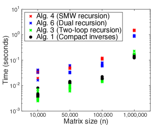
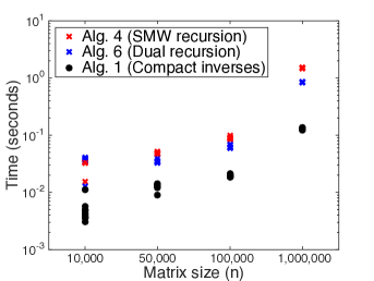
(a) $\phi=0$ (BFGS)	(b) $\phi=0.5$
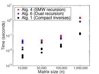
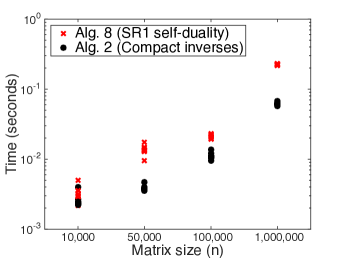
(c) $\phi=0.99$	(d) SR1

Figure 1. Semi-log plots of the computational times (in seconds) for ten runs of each of the algorithms discussed in this paper. In (a), (b), and (c), the system matrix is a member of the restricted Broyden class of updates with $\phi=0,0.5,$ and $0.99$, respectively. In (d), the system matrix is an SR1 matrix. The proposed method using compact inverses generally outperforms the other methods. Note that when $\phi=0$, our proposed method is competitive with the “two-loop recursion”, which is specific to the BFGS update.

Table 3. Relative error for Broyden class matrices with $\phi=0.00$ (BFGS).

	Two-Loop	Recursive	Recursive	Compact
$n$	Recursion	SMW	$H_{k+1}$	Inverses
	(Alg. 3)	(Alg. 4)	(Alg. 6)	(Alg. 1)
10,000	4.88e-16	4.63e-16	5.37e-16	3.59e-16
50,000	2.93e-16	4.44e-16	3.61e-16	4.20e-16
100,000	6.64e-16	3.74e-16	6.16e-16	3.81e-16
1,000,000	1.47e-15	1.46e-15	1.45e-15	1.51e-15

Table 4. Relative error for Broyden class matrices with $\phi=0.50$.

$n$	Recursive SMW	Recursive $H_{k+1}$	Compact Inverses
	(Alg. 4)	(Alg. 6)	(Alg. 1)
10,000	9.90e-16	8.37e-16	8.15e-16
50,000	4.25e-16	6.80e-16	5.82e-15
100,000	7.00e-16	6.31e-16	9.14e-16
1,000,000	2.77e-16	2.40e-16	3.56e-16

Table 5. Relative error for Broyden class matrices with $\phi=0.99$.

$n$	Recursive SMW	Recursive $H_{k+1}$	Compact Inverses
	(Alg. 4)	(Alg. 6)	(Alg. 1)
10,000	8.33e-16	1.59e-15	1.63e-15
50,000	8.45e-15	1.21e-14	3.88e-15
100,000	7.28e-14	6.67e-14	2.67e-14
1,000,000	2.59e-15	1.80e-15	3.29e-15

Table 6. Relative error for SR1 matrices.

$n$	Self-Duality	Compact Inverses
	(Alg. 8)	(Alg. 2)
10,000	1.98e-15	6.10e-15
50,000	2.24e-14	7.57e-14
100,000	5.07e-14	6.44e-14
1,000,000	8.67e-13	2.26e-12

7. Concluding Remarks

We derived the compact formulation for members of the restricted Broyden class and the SR1 update. With this compact formulation, we showed how to solve linear systems defined by limited-memory quasi-Newton matrices. Numerical results suggest that this proposed approach is efficient and accurate. This approach has two distinct advantages over existing procedures for solving limited-memory quasi-Newton systems. First, there is a natural way to use the compact formulation for the inverse to obtain the condition number of the linear system. Second, when a new quasi-Newton pair is computed, computational savings can be achieved by simple updates to the matrix factors in the compact formulation.

Future work includes integrating this linear solver inside line-search and trust-region methods for large-scale optimization.

8. Acknowledgements

The authors would like to thank Tammy Kolda for initial conversations on this subject.

Appendix A Two-loop recursion

The Broyden-Fletcher-Goldfarb-Shanno (BFGS) update is obtained by setting $\phi=0$ in (2). In this case, $B_{k+1}$ simplifies to

(38) $$B_{k+1}=B_{k}-\frac{1}{s_{k}^{T}B_{k}s_{k}}B_{k}s_{k}s_{k}^{T}B_{k}+\frac{1}{y_{k}^{T}s_{k}}y_{k}y_{k}^{T}.$$

The inverse of the BFGS matrix $B_{k+1}$ is given by

$$B_{k+1}^{-1}=\left(I-\frac{s_{k}y_{k}^{T}}{y_{k}^{T}s_{k}}\right)B_{k}^{-1}\left(I-\frac{y_{k}s_{k}^{T}}{y_{k}^{T}s_{k}}\right)+\frac{s_{k}s_{k}^{T}}{y_{k}^{T}s_{k}},$$

which can be written recursively as

(39) $$B^{-1}_{k+1} = (V_{k}^{T}\cdots V_{0}^{T})B_{0}^{-1}(V_{0}\cdots V_{k})+\frac{1}{y_{0}^{T}s_{0}}(V_{k}^{T}\cdots V_{1}^{T})s_{0}s_{0}^{T}(V_{1}\cdots V_{k})$$

$$+\frac{1}{y_{1}^{T}s_{1}}(V_{k}^{T}\cdots V_{2}^{T})s_{1}s_{1}^{T}(V_{2}\cdots V_{k})+\cdots+\frac{1}{y_{k}^{T}s_{k}}s_{k}s_{k}^{T},$$

where $V_{i}=I-\frac{1}{y_{i}^{T}s_{i}}y_{i}s_{i}^{T}$ (see, e.g., [18, p.177–178]). Solving (1) can be done efficiently using the well-known two-loop recursion [17].

$q\leftarrow z$;

for  $i=k-1,\dots,0$

     $\alpha_{i}\leftarrow(s_{i}^{T}q)/(y_{i}^{T}s_{i})$;  $q\leftarrow q-\alpha_{i}y_{i}$;

end 

$r\leftarrow B_{0}^{-1}q$;

for  $i=0,\ldots,k-1$

     $\beta\leftarrow(y_{i}^{T}r)/(y_{i}^{T}s_{i})$;   $r\leftarrow r+(\alpha_{i}-\beta)s_{i}$:

end 

ALGORITHM 3 Two-loop recursion to compute $r=B_{k}^{-1}z$ when $B_{k}$ is a BFGS matrix

Assuming that the inner products $y_{i}^{T}s_{i}$ can be precomputed and $B_{0}$ is a scalar multiple of the identity matrix, then the total operation count for Algorithm 3 is $4nk+3k+n+2k(2n-1)$ flops, which includes $2k$ vector inner products.

Appendix B SMW recursion

In the symmetric case, the SMW formula for a rank-one change is given by

(40) $$(A+\alpha uu^{T})^{-1}=A^{-1}-\frac{\alpha}{1+\alpha u^{T}A^{-1}u}A^{-1}uu^{T}A^{-1}.$$

We now show how (40) can be used to compute the inverse of $B_{k+1}$. First, for $0\leq j\leq k$, define

(41) $$\begin{array}[]{rlllrll}\alpha_{3j}&=&(y_{j}^{T}s_{j})^{-1},&\hskip 28.45274ptu_{3j}&=&y_{j},\\ \alpha_{3j+1}&=&\phi(s_{j}^{T}B_{j}s_{j}),&\hskip 28.45274ptu_{3j+1}&=&\displaystyle\frac{y_{j}}{y_{j}^{T}s_{j}}-\frac{B_{j}s_{j}}{s_{j}^{T}B_{j}s_{j}},\\ \alpha_{3j+2}&=&-(s_{j}^{T}B_{j}s_{j})^{-1},&\hskip 28.45274ptu_{3j+2}&=&B_{j}s_{j},\end{array}$$

Letting

$$C_{0}=B_{0}\quad\text{and}\quad U_{i}=\alpha_{i}u_{i}u_{i}^{T}$$

for $0\leq i\leq 3k$, we define the matrices

(42) $$C_{1}=C_{0}+U_{0},\quad C_{2}=C_{1}+U_{1},\quad\ldots,\quad C_{3(k+1)}=C_{3(k+1)-1}+U_{3(k+1)-1}.$$

By construction, $C_{3(k+1)}=B_{k+1}$. It can be shown that each $C_{i}$ is positive definite and so $u_{i}^{T}C_{i}^{-1}u_{i}>0$ for each $i$. For the restricted Broyden class, $\alpha_{3j}$ and $\alpha_{3j+1}$, $j=0,\ldots,k$ are both strictly positive. Thus, the denominator in (40) is strictly positive for the rank-one changes associated the $3j$ and $3j+1$, $j=0,\ldots k$, and thus, the SMW formula is well-defined for these rank-one updates. Since $C_{3j}=B_{j}$ and $B_{j}$ is positive definite, the rank-one update associated with $j+2$, $j=0,\ldots k$, must result in a positive-definite matrix; in other words, (40) is well defined. Thus, solving the system $B_{k+1}r=z$ is equivalent to computing $r=C_{3(k+1)}^{-1}z$. Apply the SMW formula in (40) to obtain the inverse of $C_{i+1}$ from $C_{i}^{-1}$, we obtain

(43) $$C_{i+1}^{-1}z=C_{i}^{-1}z-\frac{\alpha_{i}}{1+\alpha_{i}u_{i}^{T}C_{i}^{-1}u_{i}}C_{i}^{-1}u_{i}u_{i}^{T}C_{i}^{-1}z,$$

for $0\leq i<3(k+1).$ Recursively applying (43) to $C_{i}^{-1}z$, we obtain that

(44) $$C_{i+1}^{-1}z=C_{0}^{-1}z-\sum_{j=0}^{i}\frac{\alpha_{j}}{1+\alpha_{j}u_{j}^{T}C_{j}^{-1}u_{j}}C_{j}^{-1}u_{j}u_{j}^{T}C_{j}^{-1}z,$$

and more importantly,

(45) $$C_{3(k+1)}^{-1}z=C_{0}^{-1}z-\sum_{j=0}^{3(k+1)-1}\frac{\alpha_{j}}{1+\alpha_{j}u_{j}^{T}C_{j}^{-1}u_{j}}C_{j}^{-1}u_{j}u_{j}^{T}C_{j}^{-1}z.$$

Computing (45) can be simplified by defining the following two quantities:

(46) $$\tau_{j}=\frac{\alpha_{j}}{1+\alpha_{j}u_{j}^{T}C_{j}^{-1}u_{j}}\quad\text{and}\quad p_{j}=C_{j}^{-1}u_{j}.$$

Substituting (46) into (45) yields

(47) $$C_{3(k+1)}^{-1}z=C_{0}^{-1}z-\sum_{j=0}^{3(k+1)-1}\tau_{j}(p_{j}^{T}z)p_{j},$$

where $\tau_{j}=\alpha_{j}(1+\alpha_{j}p_{j}^{T}u_{j})^{-1}.$ The advantage of representation is that computing $C_{3(k+1)}^{-1}z$ requires only vector inner products. Moreover, the vectors $p_{j}$ can be computed by evaluating (44) at $z=u_{j}$ for $i=j-1$; that is,

$$p_{j}=C_{j}^{-1}u_{j}=C_{0}^{-1}u_{j}-\sum_{i=0}^{j-1}\tau_{i}(p_{i}^{T}u_{j})p_{i}.$$

In Algorithm 4, we present the recursion to solve the linear system $B_{k+1}r=z$ using the SMW formula (see related methods in [9, 15]). We assume $B_{0}$ is an easily-invertible initial matrix.

$r\leftarrow C_{0}^{-1}z$;

for  $j=0,\ldots,3(k+1)-1$

     if  $\mod(j,3)=0$

           $i\leftarrow j/3$;   $u\leftarrow y_{i}$;   $\alpha\leftarrow y_{i}^{T}s_{i}$;

     else if $\mod(j,3)=1$

           $i\leftarrow(j-1)/3$;  $u\leftarrow(y_{i})/(y_{i}^{T}s_{i})-(B_{i}s_{i})/(s_{i}^{T}B_{i}s_{i})$;   $\alpha\leftarrow\phi(s_{i}^{T}B_{i}s_{i})$;

      else  

           $i\leftarrow(j-2)/3$;   $u\leftarrow B_{i}s_{i}$;   $\alpha\leftarrow-(s_{i}^{T}B_{i}s_{i})^{-1}$;

     end 

     $p_{j}\leftarrow C_{0}^{-1}u$;

     for  $l=0,\ldots,j$

           $p_{j}\leftarrow p_{j}-\tau_{l}(p_{l}^{T}u)p_{l}$;

     end 

     $\tau_{j}\leftarrow\alpha/(1+\alpha p_{j}^{T}u)$;

     $r\leftarrow r-\tau_{j}(p_{j}^{T}z)p_{j}$;

end 

ALGORITHM 4 Computing $r=B_{k+1}^{-1}z$

At each iteration, Algorithm 4 computes $\alpha$ and $u$, which are defined in (41) and require matrix-vector products involving the matrices $B_{i}$ for $0\leq i\leq k$. The main difficulty in computing $\alpha$ and $u$ is the computation of matrix-vector products with the matrices $B_{i}$ for each $i$. Note that if we are able to form $u_{3j+2}=B_{j}s_{j}$, then we are able to compute all other terms that use $B_{j}s_{j}$ in (41). In what follows, we show how to compute $u_{3j+2}$ without storing $B_{i}$ for $0\leq i\leq k$. This idea is based on [18, Procedure 7.6].

We begin by writing $C_{3(k+1)}$ in (42) as follows:

$$C_{3(k+1)} = B_{0}+\sum_{j=0}^{k}\alpha_{3j}u_{3j}u_{3j}^{T}+\alpha_{3j+1}u_{3j+1}u_{3j+1}^{T}+\alpha_{3j+2}u_{3j+2}u_{3j+2}^{T},$$

where $\alpha_{i}$ and $u_{i}$ are defined by (41). Since $B_{j}=C_{3j}$, then

$$u_{3j+2} = B_{j}s_{j}$$

$$= \left(B_{0}+\sum_{i=0}^{j-1}\alpha_{3i}u_{3i}u_{3i}^{T}+\alpha_{3i+1}u_{3i+1}u_{3i+1}^{T}+\alpha_{3i+2}u_{3i+2}u_{3i+2}^{T}\right)s_{j}$$

$$= B_{0}s_{j}+\sum_{i=0}^{j-1}\alpha_{3i}(u_{3i}^{T}s_{j})u_{3i}+\alpha_{3i+1}(u_{3i+1}^{T}s_{j})u_{3i+1}+\alpha_{3i+2}(u_{3i+2}^{T}s_{j})u_{3i+2}.$$

All the terms in the above summation only involve vectors that have been previously computed. Having computed $u_{3j+2}$, it is then possible to compute $\alpha_{3j+1},\alpha_{3j+2},$ and $u_{3j+1}$. (The other terms $\alpha_{3j}$ and $u_{3j}$ do not depend on $B_{j}s_{j}$.) The following algorithm computes the terms $\alpha$ and $u$ that are used in Algorithm 4.

for  $j=0,\ldots,k$

     $u_{3j}\leftarrow y_{j}$;

     $\alpha_{3j}\leftarrow 1/(s_{j}^{T}y_{j})$;

     $u_{3j+2}\leftarrow B_{0}s_{j}+\sum_{i=0}^{j-1}\left[\alpha_{3i}(u_{3i}^{T}s_{j})u_{3i}+\alpha_{3i+1}(u_{3i+1}^{T}s_{j})u_{3i+1}+\alpha_{3i+2}(u_{3i+2}^{T}s_{j})u_{3i+2}\right]$;

     $\alpha_{3j+2}\leftarrow-1/(s_{j}^{T}u_{3j+2})$;

     $u_{3j+1}\leftarrow\alpha_{3j}y_{j}+\alpha_{3j+2}u_{3j+2}$;

     $\alpha_{3j+1}=-\phi/\alpha_{3j+2}$;

end 

ALGORITHM 5 Unrolling the limited-memory Broyden convex class formula

Assuming $s_{j}^{T}y_{j}$ is precomputed at each step, Algorithm 5 requires

$$\sum_{j=0}^{k}\big{\{}3j+1\big{\}}=\frac{3(k+1)k}{2}+k+1=\frac{(k+1)(3k+2)}{2}$$

vector inner products and

$$\sum_{j=0}^{k}\left\{1+2n+(5n+3)j+1+3n+1\right\}=\frac{(5n+3)(k+2)(k+1)}{2}$$

additional flops. With the $\alpha$’s and the $u$’s computed in Algorithm 5, the rest of Algorithm 4 requires

$$\sum_{j=0}^{3(k+1)-1}\left\{j+1+1\right\}=\frac{3(k+1)(3(k+1)+5)}{2}$$

vector inner products and

$$\sum_{j=0}^{3(k+1)-1}\left\{n+(2n+1)l+3+(2n+1)\right\} = \frac{3(k+1)(3(k+1)+1)(2n+1)}{2}$$

$$+3(k+1)(3n+4)$$

additional flops. Thus, the total number of vector inner products for Algorithm 4 is $6(k+1)^{2}+7(k+1)$ and the total flop count is

$$\frac{1}{2}(k+1)(23kn+52n+12k+42)+(2n-1)(6(k+1)^{2}+7(k+1)),$$

which includes $6(k+1)^{2}+7(k+1)$ vector inner products.

Appendix C Computing products with $H_{k+1}$ recursively

The inverse of $B_{k+1}$ in (2) is given by

$$H_{k+1}=H_{k}+\frac{1}{s_{k}^{T}y_{k}}s_{k}s_{k}^{T}-\frac{1}{y_{k}^{T}H_{k}y_{k}}H_{k}y_{k}y_{k}^{T}H_{k}+\Phi_{k}(y_{k}^{T}H_{k}y_{k})v_{k}v_{k}^{T},$$

where

$$v_{k}=\frac{s_{k}}{y_{k}^{T}s_{k}}-\frac{H_{k}y_{k}}{y_{k}^{T}H_{k}y_{k}}\quad\text{and}\quad\Phi_{k}=\frac{(1-\phi)(y_{k}^{T}s_{k})^{2}}{(1-\phi)(y_{k}^{T}s_{k})^{2}+\phi(y_{k}^{T}H_{k}y_{k})(s_{k}^{T}B_{k}s_{k})},$$

and $H_{k}\mathop{\,{\scriptstyle\stackrel{{\scriptstyle\triangle}}{{=}}}}\,B_{k}^{-1}$. Thus, the solution to $B_{k+1}r=z$ can be obtained from

$$B_{k+1}^{-1}z = \left(H_{0}z+\sum_{i=0}^{k}\frac{1}{s_{i}^{T}y_{i}}s_{i}s_{i}^{T}-\frac{1}{y_{i}^{T}H_{i}y_{i}}H_{i}y_{i}y_{i}^{T}H_{i}+\Phi_{i}(y_{i}^{T}H_{i}y_{i})v_{i}^{T}v_{i}\right)z$$

$$= H_{0}z+\sum_{i=0}^{k}\frac{s_{i}^{T}z}{s_{i}^{T}y_{i}}s_{i}-\frac{y_{k}^{T}H_{i}z}{y_{i}^{T}H_{i}y_{i}}H_{i}y_{i}+\Phi_{i}(y_{i}^{T}H_{i}y_{i})(v_{i}^{T}z)v_{i}.$$

In order to avoid storing $H_{0},\ldots,H_{k}$ for matrix-vector products, we make use of the following variables:

(48) $$\begin{array}[]{rlllrll}\alpha_{3i}&=&(s_{i}^{T}y_{i})^{-1},&\hskip 28.45274ptu_{3i}&=&s_{i},\\ \alpha_{3i+2}&=&-(y_{i}^{T}H_{i}y_{i})^{-1}&\hskip 28.45274ptu_{3i+2}&=&H_{i}y_{i},\\ \alpha_{3i+1}&=&\Phi_{i}(y_{i}^{T}H_{i}y_{i}),&\hskip 28.45274ptu_{3i+1}&=&\displaystyle\frac{s_{i}}{y_{i}^{T}s_{i}}-\frac{H_{i}y_{i}}{y_{i}^{T}H_{i}s_{i}}.\\ \end{array}$$

With these definitions, we have that

(49) $$B_{k+1}^{-1}z=H_{0}z+\sum_{i=0}^{k}\alpha_{3i}(u_{3i}^{T}z)u_{3i}+\alpha_{3i}(u_{3i+1}^{T}z)u_{3i+1}+\alpha_{3i}(u_{3i+2}^{T}z)u_{3i+2},$$

and, thus, a recursion relation can be used for matrix-vector products with $H_{0},\ldots,H_{k}$. Algorithm 6 details how to solve for $r$ in (1) using the expression for $B_{k+1}^{-1}$ in (49) without explicitly storing $H_{0},\ldots,H_{k}$.

$r\leftarrow H_{0}z$;

for  $j=0,\ldots,3(k+1)-1$

     if  $\mod(j,3)=0$

           $i\leftarrow j/3$;   $u\leftarrow s_{i}$;   $\alpha\leftarrow(y_{i}^{T}s_{i})^{-1}$;

     else if $\mod(j,3)=1$

           $i\leftarrow(j-1)/3$;   $u\leftarrow H_{i}y_{i}$;   $\alpha\leftarrow-(y_{i}^{T}H_{i}y_{i})^{-1}$;

      else  

           $i\leftarrow(j-2)/3$;   $u\leftarrow(s_{i})/(y_{i}^{T}s_{i})-(H_{i}y_{i})/(y_{i}^{T}H_{i}y_{i})$;

           $\Phi\leftarrow(1-\phi)(y_{i}^{T}s_{i})^{2}/\left((1-\phi)(y_{i}^{T}s_{i})^{2}+\phi(y_{i}^{T}H_{i}y_{i})(s_{i}^{T}B_{i}s_{i})\right)$;

           $\alpha\leftarrow\Phi(y_{i}^{T}H_{i}y_{i})$;

     end 

     $r\leftarrow r+\alpha(u^{T}z)u$;

end 

ALGORITHM 6 Computing $r=H_{k+1}z$

The following algorithm computes products involving the matrices $H_{i}$ for $0\leq i\leq k$ for use in Algorithm 6. The algorithm avoids storing any matrices, and matrix-vector products are computed recursively. The derivation of this algorithm is similar to that for Algorithm 5.

for  $j=0,\ldots,k$

     $\hat{u}_{3j}\leftarrow s_{j}$;

     $\hat{\alpha}_{3j}\leftarrow 1/(s_{j}^{T}y_{j})$;

     $\hat{u}_{3j+1}\leftarrow H_{0}y_{j}+\sum_{i=0}^{j-1}\left[\hat{\alpha}_{3i}(\hat{u}_{3i}^{T}y_{j})\hat{u}_{3i}+\hat{\alpha}_{3i+1}(\hat{u}_{3i+1}^{T}y_{j})\hat{u}_{3i+1}+\hat{\alpha}_{3i+2}(\hat{u}_{3i+2}^{T}y_{j})\hat{u}_{3i+2}\right]$;

     $\hat{\alpha}_{3j+1}\leftarrow-1/(y_{j}^{T}\hat{u}_{3j+2})$;

     $\hat{u}_{3j+2}\leftarrow\hat{\alpha}_{3j}s_{j}+\hat{\alpha}_{3j+2}\hat{u}_{3j+2}$;

     Compute $\alpha_{3j+2}$ using Algorithm 5;

     $\Phi_{j}\leftarrow(1-\phi)/(1-\phi+\phi\hat{\alpha}_{3j}^{2}/(\hat{\alpha}_{3j+1}\alpha_{3j+2}))$;

     $\hat{\alpha}_{3j+2}=-\Phi_{j}/\hat{\alpha}_{3j+1}$;

end 

ALGORITHM 7 Unrolling the limited-memory Broyden convex class formula

Assuming $s_{j}^{T}y_{j}$ is precomputed at each step, Algorithm 7 requires

$$\sum_{j=0}^{k}\left\{3j+1\right\}+\frac{(k+1)(3k+2)}{2}=(3k+2)(k+1)$$

vector inner products and

$$\sum_{j=0}^{k}\left\{1+(5n+3)j+2n+1+3n+8+1\right\}+\frac{3(k+1)(3(k+1)+5)}{2}$$

$$\quad=(5n+3)(k+1)k+(10n+14)(k+1)$$

additional flops. With the $\alpha$’s and the $u$’s computed in Algorithm 7, the rest of Algorithm 6 requires $3(k+1)$ vector inner products and $3(k+1)(2n+1)+n$ additional flops. Thus, the total flop count for Algorithm 6 is

$$(5n+3)(k+1)k+(k+1)(16n+17)+n+(2n-1)(3k+5)(k+1),$$

which includes $(3k+5)(k+1)$ vector inner products.

Appendix D Relationships between updates

We note that in the case of the BFGS update ($\phi=0$), the compact representation of the BFGS matrix is consistent with its known compact representation derived in [5]. In particular, $\tilde{M}_{k}$ in (11) simplifies to

$$\tilde{M}_{k} = (-M_{k}^{-1}-\Psi_{k}^{T}H_{0}\Psi_{k})^{-1}$$

$$= \begin{bmatrix}0&-R_{k}-D_{k}\\ -R_{k}^{T}-D_{k}&-D_{k}-Y_{k}^{T}H_{0}Y_{k}\end{bmatrix}^{-1}$$

$$= \begin{bmatrix}\bar{R}_{k}^{-T}(D_{k}+Y_{k}^{T}H_{0}Y_{k})\bar{R}_{k}^{-1}&-\bar{R}_{k}^{-T}\\ -\bar{R}_{k}^{-1}&0\end{bmatrix},$$

where $\bar{R}_{k}=R_{k}+D_{k}$. Thus, the compact representation for the inverse of a BFGS matrix is given by

(50) $$H_{k+1}=H_{0}+[\ S_{k}\ \ \ H_{0}Y_{k}\ ]\begin{bmatrix}\bar{R}_{k}^{-T}(D_{k}+Y_{k}^{T}H_{0}Y_{k})\bar{R}_{k}^{-1}&-\bar{R}_{k}^{-T}\\ -\bar{R}_{k}^{-1}&0\end{bmatrix}\begin{bmatrix}S_{k}^{T}\\ Y_{k}^{T}H_{0}\end{bmatrix},$$

which is equivalent to that found in [5, Equation (2.6)].

When $\phi=1$, then $B_{k+1}$ in (2) is known as the Davidon-Fletcher-Powell (DFP) update, which preceded the BFGS update. The BFGS and DFP formulas are known to be duals of each other, meaning one update can be obtained from the other by interchanging $s_{k}$ with $y_{k}$ and $B_{k}$ with $H_{k}$. Here, we demonstrate explicitly that the compact representation of the BFGS and DFP updates are also duals of each other. In addition, we show that the compact representation of the SR1 matrix is self-dual.

Consider the compact formulation for the inverse of a BFGS matrix (i.e., $\phi=0$) in (50). This is equivalent to

$$H_{k+1} = H_{0}+[\ H_{0}Y_{k}\ \ \ S_{k}\ ]\begin{bmatrix}0&-\bar{R}_{k}^{-1}\\ -\bar{R}_{k}^{-T}&\bar{R}_{k}^{-T}(D_{k}+Y_{k}^{T}H_{0}Y_{k})\bar{R}_{k}^{-1}\end{bmatrix}\begin{bmatrix}Y_{k}^{T}H_{0}\\ S_{k}^{T}\end{bmatrix}$$

$$= H_{0}-[\ H_{0}Y_{k}\ \ \ S_{k}\ ]\begin{bmatrix}Y_{k}^{T}H_{0}Y_{k}+D_{k}&\bar{R}_{k}^{T}\\ \bar{R}_{k}&0\end{bmatrix}^{-1}\begin{bmatrix}Y_{k}^{T}H_{0}\\ S_{k}^{T}\end{bmatrix}.$$

Now we consider interchanging $B_{0}$ with $H_{0}$ and $Y_{k}$ with $S_{k}$. Notice that if $S_{k}$ and $Y_{k}$ are interchanged then the upper triangular part of $S_{k}^{T}Y_{k}$ corresponds to the lower triangular part of $Y_{k}^{T}S_{k}$, implying that $L_{k}$ and $R_{k}$ must also be interchanged. Putting this all together yields:

$$B_{k+1} = B_{0}-[\ B_{0}S_{k}\ \ \ Y_{k}\ ]\begin{bmatrix}S_{k}^{T}B_{0}S_{k}+D_{k}&(L_{k}+D_{k})^{T}\\ L_{k}+D_{k}&0\end{bmatrix}^{-1}\begin{bmatrix}S_{k}^{T}B_{0}\\ Y_{k}^{T}\end{bmatrix},$$

which is the compact formulation for a DFP matrix (see [8, Theorem 1]). In other words, the compact representations of BFGS and DFP are complementary updates of each other.

For the DFP update, $\Lambda_{k}=-D_{k}$ in (7) since $\phi=1$. Thus, the compact formulation for the inverse of a DFP matrix is given by

$$H_{k+1} = H_{0}+[\ S_{k}\ \ \ H_{0}Y_{k}]\begin{bmatrix}\ \ D_{k}&-R_{k}\\ -R_{k}^{T}&-Y_{k}^{T}H_{0}Y_{k}\end{bmatrix}^{-1}\begin{bmatrix}S_{k}^{T}\\ Y_{k}^{T}H_{0}\end{bmatrix}$$

$$= H_{0}-[\ H_{0}Y_{k}\ \ \ S_{k}]\begin{bmatrix}Y_{k}^{T}H_{0}Y_{k}&\ \ R_{k}^{T}\ \\ R_{k}&-D_{k}\ \end{bmatrix}^{-1}\begin{bmatrix}Y_{k}^{T}H_{0}\\ S_{k}^{T}\end{bmatrix}.$$

Interchanging $H_{0}$ with $B_{0}$ and $S_{k}$ with $Y_{k}$ (and $R_{k}$ with $L_{k}$) yields

$$B_{k+1}=B_{0}-[\ B_{0}S_{k}\ \ \ Y_{k}]\begin{bmatrix}S_{k}^{T}B_{0}S_{k}&\ \ L_{k}^{T}\ \\ L_{k}&-D_{k}\ \end{bmatrix}\begin{bmatrix}S_{k}^{T}B_{0}\\ Y_{k}^{T}\end{bmatrix},$$

which is the compact formulation of the BFGS matrix (see Eq. (2.17) in [5].

Finally, it is worth noting that the inverse of compact formulation for an SR1 matrix is self-dual in the sense of Section 5.2. That is, replacing $H_{0}$ with $B_{0}$ and $S_{k}$ with $Y_{k}$ (and, thus, $R_{k}$ with $L_{k}$) in (35) yields the compact formulation for the SR1 matrix given by (34).

Appendix E Solves with SR1 matrices.

The SR1 update is remarkable in that it is self-dual: initializing with $B_{0}^{-1}$ instead of $B_{0}$, replacing $s_{k}$ with $y_{k}$, and replacing $y_{k}$ with $s_{k}$ for all $k$ in (33) results in $B_{k+1}^{-1}$ (see e.g., [18]). Thus, $r=B_{k+1}^{-1}z$ can be computed using recursion (see Algorithm E.1). The first loop of Algorithm E.1 computes $p_{i}\mathop{\,{\scriptstyle\stackrel{{\scriptstyle\triangle}}{{=}}}}\,s_{i}-H_{i}y_{i}$ for $i=0,\ldots k$; the final line of Algorithm E.1 computes $r=B_{k+1}^{-1}z=B_{0}^{-1}z+\sum_{i=0}^{k}(p_{i}^{T}z)/(p_{i}^{T}y_{i})p_{i}$.

for  $i=0,\ldots k$

     $p_{i}=s_{i}-H_{0}y_{i}$;

     for $j=0\ldots i-1$

           $p_{i}=p_{i}-((p_{j}^{T}y_{i})/(p_{j}^{T}y_{j}))p_{j}$;

     end 

end

$r\leftarrow H_{0}z+\sum_{i=0}^{k}((p_{i}^{T}z)/(p_{i}^{T}y_{i}))p_{i}$;

ALGORITHM 8 Computing $r=B_{k+1}^{-1}z,$ when $B_{k+1}$ is an SR1 matrix

Thus, in the case of SR1 updates, solving linear systems with SR1 matrices can be performed using vector inner products; the cost for solving linear systems with an SR1 matrix is the same as the cost of computing products with an SR1 matrix, which can be done with

$$\left\{\sum_{i=0}^{k}i\right\}+k+1=\frac{(k+2)(k+1)}{2}$$

vector inner products and

$$\left\{\sum_{i=0}^{k}2n+(2n+1)i\right\}+2n+(k+1)(1+n)=\frac{(k+1)}{2}\left(k(2n+1)+2(3n+1)\right)+2n$$

additional flops. It should be noted that unlike members of the restricted Broyden class, SR1 matrices can be indefinite, and in particular, numerically singular. Methods found in [3, 10] can be used to compute the eigenvalues (and thus, the condition number) of SR1 matrices before performing linear solves to help avoid solving ill-conditioned systems.

Appendix F Calculations in Lemma 1.

The determinant of (12) is given by

$$\tilde{\alpha}_{0}\tilde{\delta}_{0}-\tilde{\beta}_{0}^{2} = -\frac{1-\Phi_{0}}{(s_{0}^{T}y_{0})(y_{0}^{T}H_{0}y_{0})}-\frac{\Phi_{0}(1-\Phi_{0})}{(s_{0}^{T}y_{0})^{2}}-\frac{\Phi_{0}^{2}}{(s_{0}^{T}y_{0})^{2}}$$

$$= -\frac{\phi s_{0}^{T}B_{0}s_{0}}{\Delta_{0}s_{0}^{T}y_{0}}-\frac{1-\phi}{\Delta_{0}}$$

$$= \frac{1}{\Delta_{0}}\left(\frac{s_{0}^{T}B_{0}s_{0}}{\lambda_{0}}\right),$$

where $\lambda_{0}$ in (16) is defined in (7). Thus, the first entry of (15) is given by

$$\frac{\tilde{\delta}_{0}}{\tilde{\alpha}_{0}\tilde{\delta}_{0}-\tilde{\beta}_{0}^{2}}=-\frac{\phi(s_{0}^{T}B_{0}s_{0})}{\Delta_{0}}\frac{\Delta_{0}\lambda_{0}}{s_{0}^{T}B_{0}s_{0}}=-\phi\lambda_{0}.$$

The off-diagonal elements of the right-hand side of (15) simplify as follows:

$$\frac{\tilde{\beta}_{0}}{\tilde{\alpha}_{0}\tilde{\delta}_{0}-\tilde{\beta}_{0}^{2}} = -\left(\frac{(1-\phi)(s_{0}^{T}y_{0})}{\Delta_{0}}\right)\left({\Delta_{0}}\left(\frac{\lambda_{0}}{s_{0}^{T}B_{0}s_{0}}\right)\right)$$

$$= -\frac{(1-\phi)s_{0}^{T}y_{0}}{-(1-\phi)-\displaystyle\phi\frac{s_{0}^{T}B_{0}s_{0}}{s_{0}^{T}y_{0}}}$$

$$= -\frac{(1-\phi)(s_{0}^{T}y_{0})^{2}+\phi s_{0}^{T}B_{0}s_{0}(s_{0}^{T}y_{0})-\phi s_{0}^{T}B_{0}s_{0}(s_{0}^{T}y_{0})}{-(1-\phi)s_{0}^{T}y_{0}-\phi s_{0}^{T}B_{0}s_{0}}$$

$$= s_{0}^{T}y_{0}+\phi\frac{s_{0}^{T}B_{0}s_{0}(s_{0}^{T}y_{0})}{-(1-\phi)s_{0}^{T}y_{0}-\phi s_{0}^{T}B_{0}s_{0}}$$

$$= s_{0}^{T}y_{0}+\phi\lambda_{0}.$$

Finally, the last entry of (15) can be simplified as follows:

$$\frac{\tilde{\alpha}_{0}}{\tilde{\alpha}_{0}\tilde{\delta}_{0}-\tilde{\beta}_{0}^{2}} = \frac{1}{s_{0}^{T}y_{0}}\frac{\Delta_{0}\lambda_{0}}{s_{0}^{T}B_{0}s_{0}}+(1-\phi)y_{0}^{T}H_{0}y_{0}\frac{\lambda_{0}}{s_{0}^{T}B_{0}s_{0}}$$

$$= \frac{\lambda_{0}}{(s_{0}^{T}y_{0})(s_{0}^{T}B_{0}s_{0})}\bigg{(}\Delta_{0}+(1-\phi)(y_{0}^{T}H_{0}y_{0})(s_{0}^{T}y_{0})\bigg{)}$$

$$= \frac{1}{-(1-\phi)s_{0}^{T}y_{0}-\phi s_{0}^{T}B_{0}s_{0}}\bigg{(}\Delta_{0}+(1-\phi)(y_{0}^{T}H_{0}y_{0})(s_{0}^{T}y_{0})\bigg{)}$$

$$= \frac{(1-\phi)(s_{0}^{T}y_{0})^{2}+\phi(y_{0}^{T}H_{0}y_{0})(s_{0}^{T}B_{0}s_{0})+(1-\phi)(y_{0}^{T}H_{0}y_{0})(s_{0}^{T}y_{0})}{-(1-\phi)s_{0}^{T}y_{0}-\phi(s_{0}^{T}B_{0}s_{0})}$$

$$= \frac{(1-\phi)(s_{0}^{T}y_{0})^{2}+\phi(s_{0}^{T}B_{0}s_{0})(s_{0}^{T}y_{0})}{-(1-\phi)s_{0}^{T}y_{0}-\phi(s_{0}^{T}B_{0}s_{0})}-\frac{\phi(s_{0}^{T}B_{0}s_{0})(s_{0}^{T}y_{0})}{-(1-\phi)s_{0}^{T}y_{0}-\phi(s_{0}^{T}B_{0}s_{0})}$$

$$\quad+\frac{\phi(y_{0}^{T}H_{0}y_{0})(s_{0}^{T}B_{0}s_{0})+(1-\phi)(y_{0}^{T}H_{0}y_{0})s_{0}^{T}y_{0}}{-(1-\phi)s_{0}^{T}y_{0}-\phi(s_{0}^{T}B_{0}s_{0})}$$

$$= -s_{0}^{T}y_{0}-\phi\lambda_{0}-y_{0}^{T}H_{0}y_{0}.$$

References

• [1] J.Β Brust, O.Β Burdakov, J.Β B. Erway, R.Β F. Marcia, and Y.-x. Yuan, Shape-changing L-SR1 trust-region methods. Submitted.
• [2] J.Β Brust, J.Β B. Erway, and R.Β F. Marcia, On solving L-SR1 trust-region subproblems.
• [3] O.Β Burdakov, L.Β Gong, Y.-X. Yuan, and S.Β Zikrin, On efficiently combining limited memory and trust-region techniques, Tech. Rep. 2013:13, LinkΓΆping University, The Institute of Technology, 2013.
• [4] R.Β H. Byrd, D.Β C. Liu, and J.Β Nocedal, On the behavior of broyden’s class of quasi-newton methods, SIAM Journal on Optimization, 2 (1992), pp.Β 533–557.
• [5] R.Β H. Byrd, J.Β Nocedal, and R.Β B. Schnabel, Representations of quasi-Newton matrices and their use in limited-memory methods, Math. Program., 63 (1994), pp.Β 129–156.
• [6] A.Β R. Conn, N.Β I.Β M. Gould, and P.Β L. Toint, Trust-Region Methods, Society for Industrial and Applied Mathematics (SIAM), Philadelphia, PA, 2000.
• [7] J.Β E. Dennis, Jr and J.Β J. MorΓ©, Quasi-newton methods, motivation and theory, SIAM Review, 19 (1977), pp.Β 46–89.
• [8] J.Β B. Erway, V.Β Jain, and R.Β F. Marcia, Shifted limited-memory DFP systems, in 2013 Asilomar Conference on Signals, Systems and Computers, Nov 2013, pp.Β 1033–1037.
• [9] J.Β B. Erway and R.Β F. Marcia, Limited-memory BFGS systems with diagonal updates, Linear Algebra and its Applications, 437 (2012), pp.Β 333–344.
• [10] J.Β B. Erway and R.Β F. Marcia, On efficiently computing the eigenvalues of limited-memory quasi-newton matrices, SIAM Journal on Matrix Analysis and Applications, 36 (2015), pp.Β 1338–1359.
• [11] G.Β H. Golub and C.Β F. Van Loan, Matrix Computations, The Johns Hopkins University Press, Baltimore, Maryland, thirdΒ ed., 1996.
• [12] I.Β Griva, S.Β G. Nash, and A.Β Sofer, Linear and nonlinear programming, Society for Industrial and Applied Mathematics, Philadelphia, 2009.
• [13] W.Β Huang, K.Β A. Gallivan, and P.-A. Absil, A broyden class of quasi-newton methods for riemannian optimization, SIAM Journal on Optimization, 25 (2015), pp.Β 1660–1685.
• [14] C.Β Liu and S.Β A. VanderΒ Wiel, Statistical quasi-newton: A new look at least change, SIAM Journal on Optimization, 18 (2007), pp.Β 1266–1285.
• [15] K.Β S. Miller, On the Inverse of the Sum of Matrices, Mathematics Magazine, 54 (1981), pp.Β 67–72.
• [16] J.Β L. Morales and J.Β Nocedal, Automatic preconditioning by limited memory quasi-newton updating, SIAM Journal on Optimization, 10 (2000), pp.Β 1079–1096.
• [17] J.Β Nocedal, Updating quasi-Newton matrices with limited storage, Mathematics of Computation, 35 (1980), pp.Β 773–782.
• [18] J.Β Nocedal and S.Β J. Wright, Numerical Optimization, Springer-Verlag, New York, secondΒ ed., 2006.
• [19] D.Β P. O’Leary and A.Β Yeremin, The linear algebra of block quasi-newton algorithms, Linear Algebra and Its Applications, 212 (1994), pp.Β 153–168.
• [20] Y.Β Zhang and R.Β Tewarson, Quasi-newton algorithms with updates from the preconvex part of broyden’s family, IMA Journal of Numerical Analysis, 8 (1988), pp.Β 487–509.