Symmetry Adapted Coherent States for Three-Level Atoms Interacting with One-Mode Radiation

Abstract

We introduce a combination of coherent states as variational test functions for the atomic and radiation sectors to describe a system of $N_{a}$ three-level atoms interacting with a one-mode quantised electromagnetic field, with and without the rotating wave approximation, which preserves the symmetry presented by the Hamiltonian. These provide us with the possibility of finding analytical solutions for the ground and first excited states. We study the properties of these solutions for the $V$-configuration in the double resonance condition, and calculate the expectation values of the number of photons, the atomic populations, the total number of excitations, and their corresponding fluctuations. We also calculate the photon number distribution and the linear entropy of the reduced density matrix to estimate the entanglement between matter and radiation. For the first time, we exhibit analytical expressions for all of these quantities, as well as an analytical description for the phase diagram in parameter space, which distinguishes the normal and collective regions, and which gives us all the quantum phase transitions of the ground state from one region to the other as we vary the interaction parameters (the matter-field coupling constants) of the model, in functional form.

1 Introduction

Two-level systems have been extensively studied in quantum optics [1, 2]. The promise that qutrits and qudits in general can extend the possibilities of $2$-level systems in quantum information and other scenarios makes the study of higher-dimensional quantum systems, in particulat $3$- and $4$-level systems, interesting.

Implementations of qutrit channels have been demonstrated where two photon-polarization-qubits form a biphotonic qutrit [3] and, though difficult in practice, biphoton-photon entanglement has proved manageable [4].

There has been detailed research on the physical phenomena involving two-photon processes in one three-level atom [5, 6, 7]. More recently, there has been interest in the phase states of a three-level atom interacting through one and two modes of radiation [8, 10]. Phase transitions in two-color superradiance has been discussed in [11] for the $\Lambda$-configuration. The influence of a Kerr-like medium on the temporal evolution of the second-order correlation function for a $3$-level atom has been studied in all configurations [12]. The quantum phase diagrams of three-level atoms interacting with a one-mode radiation field have been obtained analytically, for all the configurations and in the rotating wave approximation (RWA) in [13, 14].

In this paper we review the calculation of the energy surface of $3$-level atoms interacting with a one mode radiation field, with and without the RWA approximation. The energy surface is defined by the expectation value of the Hamiltonian with respect to the product of Weyl-Heisenberg coherent states for the field and the totally symmetric U($3$) coherent states for the matter. The analytical form of these energy surfaces allows us to:

i)

extend the quantum phase diagrams obtained with the RWA for the transition from the normal to the superradiant regimes of the atoms to the full Hamiltonian.

ii)

construct symmetry-adapted states that give a better description of the ground state of the system, and additionally to have an approximation to the first excited state.

These new states allow to properly determine the entanglement between matter and radiation, and the statistical behaviour of the total number of excitations operator. In section 2 we establish the Hamiltonian of the system in terms of bosonic operators for the field and U($3$) generators for the matter. We determine the energy surface, with and without the RWA approximation, calculating the expectation value of the corresponding Hamiltonians with respect to matter and field coherent states, and we describe how to use it as an approximation of the ground state of the system, in section 3. Establishing a relation between both energy surfaces allows us to extend the analytical results of the quantum phase diagrams obtained in [13, 14]. In section 4 we give the minima of the full Hamiltonian energy surface (with respect to the standard product of coherent states) for the $V$-configuration under the double resonance condition. These minima are substituted into the general expressions for the energy surface and other observables. As an example we present the results obtained for the mean square deviation of the number of photons. In section 5 we show that the model Hamiltonian in the RWA approximation has the total number of excitations operator $\mathbf{M}$ as a constant of motion while the full Hamiltonian has only the parity operator $e^{i\,\pi\,\mathbf{M}}$ as a constant of motion. These results lead us to introduce the symmetry-adapted coherent states (SACS) for the model without the RWA approximation. At the end of the section we give the corresponding energy surfaces of the model Hamiltonian for the normal and collective regimes, and for the even and odd parity cases. In section 6 we compare the results obtained for the SACS energy surface with the coherent energy surface. The same is done for other matter and field observables as well as for the photon number distribution. In particular, our methodology allows us to calculate the matter-field entanglement of the system for the SACS and compare the result with the linear entropy for the coherent states. Finally we give a summary of the obtained results.

2 The Model

We consider a system composed of $N_{a}$ three-level atoms interacting with a one-mode of quantised electromagnetic field in a cavity. The interaction occurs only through the atomic electric dipole moment, i.e., the electric quadrupole and magnetic dipole interactions are smaller by a factor of the fine structure constant $\alpha\approx 1/137$, and are thus neglected. We also use the long-wavelength approximation, i.e., the size of an atom is much smaller than the wavelength of the electromagnetic radiation. Then the full Hamiltonian model for this system is given by [5]

$$\mathbf{H}=\Omega\,\mathbf{a}^{\dagger}\mathbf{a}+\sum_{j=1}^{3}\,\omega_{j}\,\mathbf{A}_{jj}-\sum_{j<k}^{3}\frac{\mu_{jk}}{\sqrt{N_{a}}}\left(\mathbf{a}^{\dagger}+\mathbf{a}\right)\left(\mathbf{A}_{jk}+\mathbf{A}_{kj}\right)\ .$$ (1)

In this equation, $\mathbf{a}^{\dagger}$ and $\mathbf{a}$ denote the creation and annihilation operators of the one-mode radiation field of frequency $\Omega$, $\mathbf{A}_{ij}$ denotes the collective matter operators defined by $\mathbf{A}_{ij}:=\sum_{r=1}^{N_{a}}\mathbf{A}_{ij}^{(r)}$, where $\mathbf{A}_{ij}^{(r)}$ stands for the atomic operator which changes the atom $r$ from level $j$ to level $i$, the atomic levels are ordered such that $\omega_{1}\leq\omega_{2}\leq\omega_{3}$, and $\mu_{ij}$ denote the dipolar intensities. A particular atomic configuration is set by properly choosing one dipolar parameter $\mu_{ij}=0$. This Hamiltonian describes a dilute gas whose atoms only interact through the radiation field.

The collective operators $\mathbf{A}_{ij}$ satisfy the commutation relations of the $U(3)$ Lie algebra

$$\Big{[}\mathbf{A}_{ij},\,\mathbf{A}_{kl}\Big{]}=\delta_{jk}\,\mathbf{A}_{il}-\delta_{il}\,\mathbf{A}_{kj}\ ,$$ (2)

and the linear and quadratic invariants are given by

$$\mathbf{N_{a}}=\sum_{k=1}^{3}\mathbf{A}_{kk}\,,\qquad\mathbf{N^{2}_{a}}+2\,\mathbf{N_{a}}=\sum_{k,j=1}^{3}\mathbf{A}_{kj}\ \mathbf{A}_{jk}\,,$$ (3)

where $N_{a}$ denotes the number of atoms of the system.

2.1 Symmetric coherent states for the matter

If we consider a system of identical atoms, we can represent the collective atomic operators $\mathbf{A}_{ij}$ in the form

$$\mathbf{A}_{ij}=\mathbf{b}_{i}^{\dagger}\,\mathbf{b}_{j}\ ,$$ (4)

where the creation $\mathbf{b}^{\dagger}_{i}$ and annihilation $\mathbf{b}_{j}$ operators with $i,\,j=1,2,3$ satisfy the commutation relations

$$\left[\mathbf{b}_{j},\,\mathbf{b}_{k}^{\dagger}\right]=\delta_{jk}\,\mathbf{1}\ ,\quad\left[\mathbf{b}_{j},\,\mathbf{b}_{k}\right]=0\ ,\quad\left[\mathbf{b}_{j}^{\dagger},\,\mathbf{b}_{k}^{\dagger}\right]=0\ ,\quad j,\,k=1,\,2,\,3\ .$$ (5)

If we define the operators

$$\mathbf{\Gamma}^{\dagger}(\gamma):=\frac{1}{\sqrt{\sum_{k}|\gamma_{k}|^{2}}}\sum_{j=1}^{3}\,\gamma_{j}\,\mathbf{b}_{j}^{\dagger}\ ,\quad\mathbf{\Gamma}(\gamma):=\frac{1}{\sqrt{\sum_{k}|\gamma_{k}|^{2}}}\sum_{j=1}^{3}\,\gamma_{j}^{\ast}\,\mathbf{b}_{j}\ ,$$ (6)

which satisfy the commutation relations of boson operators, then it is straightforward to define the condensate or totally symmetric $U(3)$-coherent state of $N_{a}$ atoms as follows:

$$|N_{a};\,\gamma\rangle := \frac{1}{\sqrt{N_{a}!}}\,\left[\mathbf{\Gamma}^{\dagger}(\gamma)\right]^{N_{a}}\,|0\rangle=\frac{1}{(\sum_{k}|\gamma_{k}|^{2})^{N_{a}/2}}|N_{a};\,\gamma\}\ ,$$ (7)

where in the last expression we defined the unnormalised coherent state which can be written as [15]

$$|N_{a};\,\gamma\} = \sum_{n_{1}+n_{2}+n_{3}=N_{a}}\sqrt{\frac{N_{a}!}{n_{1}!\,n_{2}!\,n_{3}!}}\,\gamma_{1}^{n_{1}}\,\gamma_{2}^{n_{2}}\,\gamma_{3}^{n_{3}}\,|n_{1},\,n_{2},\,n_{3}\rangle\ ,$$

and where $|n_{1},\,n_{2},\,n_{3}\rangle$ denotes the state with $n_{i}$ atoms in levels $i=1,\,2,\,3$. In these expressions $\gamma$ stands for $(\gamma_{1},\,\gamma_{2},\,\gamma_{3})$.

The scalar product of these states is

$$\{N_{a};\,\gamma|N_{a}^{\prime};\,\gamma^{\prime}\}=\delta_{N_{a}\,N_{a}^{\prime}}\,\left(\gamma^{\ast}\cdot\gamma^{\prime}\right)^{N_{a}}\ ,$$ (8)

with

$$\gamma^{\ast}\cdot\gamma^{\prime}=\sum_{j=1}^{3}\,\gamma_{j}^{\ast}\,\gamma^{\prime}_{j}\ .$$

The $U(3)$ Lie algebra generators can be represented in this basis by the differential operators

$$\mathbf{A}_{jk}:=\mathbf{b}_{j}^{\dagger}\mathbf{b}_{k}\longmapsto\gamma_{j}^{\ast}\,\frac{\partial\phantom{\gamma_{j}^{\ast}}}{\gamma_{k}^{\ast}}\ .$$ (9)

This result allows us to obtain the matrix elements of the generators $A_{jk}$ in the unnormalised coherent states:

$$\{N_{a};\,\gamma|\mathbf{A}_{jk}|N_{a}^{\prime};\,\gamma^{\prime}\}=N_{a}\,\frac{\gamma_{j}^{\ast}\,\gamma^{\prime}_{k}}{\gamma^{\ast}\cdot\gamma^{\prime}}\,\{N_{a};\,\gamma|N_{a}^{\prime};\,\gamma^{\prime}\}\ ,\quad\gamma^{\ast}\cdot\gamma^{\prime}\not=0\ .$$ (10)

The matrix elements of operator $A_{ij}A_{kl}$ can also be calculated using this method and the result is given by

$$\{N_{a};\,\gamma|\,\mathbf{A}_{ij}\,\mathbf{A}_{kl}\,|\,N_{a}^{\prime};\,\gamma^{\prime}\} = \frac{N_{a}\,\gamma_{i}^{\ast}\,\gamma^{\prime}_{l}}{\gamma^{\ast}\cdot\gamma^{\prime}}\Big{[}\,(N_{a}-1)\,\frac{\gamma^{\prime}_{j}\,\gamma_{k}^{\ast}}{(\gamma^{\ast}\cdot\gamma^{\prime})}+\delta_{jk}\,\Big{]}\,\{N_{a};\,\gamma|\,N_{a}^{\prime};\,\gamma^{\prime}\}\ .$$ (11)

In the normalised coherent states we can divide numerator and denominator by $\gamma_{1}$, and this quantity will not appear in the final expressions. The same can be done for the matrix elements of the $U(3)$ generators between coherent states. This shows that the introduced coherent states actually depend only on two complex variables instead of three. We will keep the redundant expression $\gamma=(\gamma_{1},\,\gamma_{2},\,\gamma_{3})$ to simplify the notation. However, we must set $\gamma_{1}=1$. Also, because atomic coherent states with different number of atoms are orthogonal, we will consider always the same number of atoms $N_{a}$ and drop this number from the labelling of the states.

3 Energy Surface

In order to study the ground state of the Hamiltonian (1), we calculate its energy surface which is defined as the expectation value with respect to

$$|\alpha;\,\gamma\}:=|\alpha\}\otimes|\,\gamma\}\ .$$ (12)

Here we use also the unnormalised Weyl–Heisenberg coherent states

$$|\alpha\}:=\exp\left(\alpha\,\mathbf{a}^{\dagger}\right)\,|0\rangle\ .$$ (13)

Thus, the energy surface has the form

$$E(\alpha,\,\gamma):=\{\alpha;\,\gamma|\,\mathbf{H}\,|\alpha;\,\gamma_{2},\,\gamma_{3}\}/\{\alpha;\,\gamma|\alpha;\,\gamma\}$$

$$\ =\Omega\,\left|\alpha\right|^{2}+\frac{1}{\gamma^{\ast}\cdot\gamma}\Big{\{}\,N_{a}\,\sum_{i=1}^{3}\omega_{i}\,\left|\gamma_{i}\right|^{2}-\sqrt{N_{a}}\,\sum_{i<j}^{3}\mu_{ij}\,\left(\gamma_{i}^{\ast}\gamma_{j}+\gamma_{j}^{\ast}\gamma_{i}\right)\,\left(\alpha^{\ast}+\alpha\right)\Big{\}}\ .$$ (14)

Using the polar form of the complex numbers

$$\alpha:=\varrho\,\exp(i\,\varphi)\ ,\quad\gamma_{j}:=\varrho_{j}\,\exp(i\,\varphi_{j})\ ,\ j=1,\,2,\,3\ ,$$ (15)

and setting $\gamma_{1}=1$, this function takes the form

$$E(\varrho,\,\varphi,\,\varrho_{j},\,\varphi_{j})=\Omega^{2}\,\varrho^{2}+\Big{\{}N_{a}\,\Big{[}\omega_{1}+\omega_{2}\,\varrho_{2}^{2}+\omega_{3}\,\varrho_{3}^{2}\Big{]}-4\,\sqrt{N_{a}}\Big{[}\,\mu_{12}\,\varrho_{2}\,\cos\varphi_{2}$$

$$\quad+\mu_{13}\,\varrho_{3}\,\cos\varphi_{3}+\mu_{23}\,\varrho_{2}\,\varrho_{2}\,\cos(\varphi_{2}-\varphi_{3})\Big{]}\,\varrho\,\cos\varphi\Big{\}}/\left(1+\varrho_{2}^{2}+\varrho_{3}^{2}\right)\ .$$ (16)

If we assume that the interaction intensities $\mu_{ij}$ are non-negative numbers, the minimum value of this energy surface is obtained when the angles satisfy the conditions

$$\cos\varphi_{2}\,\cos\varphi=\cos\varphi_{3}\,\cos\varphi=\cos(\varphi_{2}-\varphi_{3})\,\cos\varphi\equiv 1\ ,$$ (17)

because in this case the contribution of the atom-field interaction Hamiltonian diminishes the value of the energy surface. Actually, this results from considering the hessian of the Hamiltonian; in any case the product of these cosines times the dipolar intensity parameter must be positive in order to have a minimum. Thus

$$E_{min}(\varrho_{c},\,\varrho_{2\,c},\,\varrho_{3\,c})=\Omega\,\varrho_{c}^{2}+\Big{\{}N_{a}\,\Big{[}\omega_{1}+\omega_{2}\,\varrho_{2\,c}^{2}+\omega_{3}\,\varrho_{3\,c}^{2}\Big{]}$$

$$\qquad\qquad\quad-4\,\sqrt{N_{a}}\,\varrho_{c}\Big{[}\mu_{12}\,\varrho_{2\,c}+\mu_{13}\,\varrho_{3\,c}+\mu_{23}\,\varrho_{2\,c}\,\varrho_{3\,c}\Big{]}\Big{\}}/\left(1+\varrho_{2\,c}^{2}+\varrho_{3\,c}^{2}\right)\,,$$ (18)

where $\varrho_{c}$, $\varrho_{2\,c}$ and $\varrho_{3\,c}$ denote the minima critical values of the corresponding variables.

3.1 Comparison with the RWA Hamiltonian

The energy surface of the Hamiltonian in the rotating wave approximation is given by

$$E_{\hbox{\tiny{RWA}}}(\alpha,\,\gamma)=\Omega\left|\alpha\right|^{2}+\frac{1}{\gamma^{\ast}\cdot\gamma}\Big{\{}N_{a}\sum_{i=1}^{3}\omega_{i}\left|\gamma_{i}\right|^{2}-\sqrt{N_{a}}\sum_{i<j}^{3}\mu_{ij}\left(\gamma_{i}^{\ast}\,\gamma_{j}\,\alpha^{\ast}+\gamma_{j}^{\ast}\,\gamma_{i}\alpha\right)\Big{\}}.$$ (19)

Using polar coordinates (15) we get

$$E_{\hbox{\tiny{RWA}}}(\varrho,\,\varphi,\,\varrho_{j},\,\varphi_{j})=\Omega^{2}\,\varrho^{2}+\Big{\{}N_{a}\Big{[}\omega_{1}+\omega_{2}\,\varrho_{2}^{2}+\omega_{3}\,\varrho_{3}^{2}\Big{]}-2\,\sqrt{N_{a}}\,\varrho\Big{[}\mu_{12}\,\varrho_{2}\cos(\varphi_{2}-\varphi)$$

$$\qquad+\mu_{13}\,\varrho_{3}\,\cos(\varphi_{3}-\varphi)+\mu_{23}\,\varrho_{2}\,\varrho_{2}\,\cos(\varphi_{3}-\varphi_{2}-\varphi)\Big{]}\,\Big{\}}/\left(1+\varrho_{2}^{2}+\varrho_{3}^{2}\right)\ .$$ (20)

In this case the minimum value of the energy surface is found when the angles satisfy the conditions

$$\cos(\varphi_{2}-\varphi)=\cos(\varphi_{3}-\varphi)=\cos(\varphi_{3}-\varphi_{2}-\varphi)\equiv 1\ ,$$ (21)

and its expression is

$$\left(E_{\hbox{\tiny{RWA}}}\right)_{min}(\varrho_{c},\,\varrho_{2\,c},\,\varrho_{3\,c})=\Omega\,\varrho_{c}^{2}+\Big{\{}N_{a}\,\Big{[}\omega_{1}+\omega_{2}\,\varrho_{2\,c}^{2}+\omega_{3}\,\varrho_{3\,c}^{2}\Big{]}$$

$$\qquad-2\,\sqrt{N_{a}}\,\varrho\,\Big{[}\mu_{12}\,\varrho_{2\,c}+\mu_{13}\,\varrho_{3\,c}+\mu_{23}\,\varrho_{2\,c}\,\varrho_{3\,c}\Big{]}\Big{\}}/\left(1+\varrho_{2\,c}^{2}+\varrho_{3\,c}^{2}\right)\ .$$ (22)

Comparing this equation with Eq. (18) we note that the energy surfaces $E_{min}$ and $(E_{\hbox{\tiny{RWA}}})_{min}$ coincide if we carry out the following identification of the atom-field interaction parameters:

$$\left(\mu_{jk}\right)_{\hbox{\tiny{RWA}}}\longrightarrow 2\,\left(\mu_{jk}\right)\ .$$ (23)

Said differently, $E_{\hbox{\tiny{RWA}}}$ will inherit the properties of $E_{min}$ at values of $(\mu_{ij})_{\hbox{\tiny{RWA}}}$ equal to $\frac{1}{2}\mu_{ij}$.

We want to emphasize that equation (23) is valid for all the atomic configurations. Therefore the analytic expressions for the quantum phase diagrams of the model Hamiltonian with the RWA approximation can be now extended to the full Hamiltonian, i.e., in equations (5)-(7) of [13] or equations (36)-(38) of [14] we properly substitute the dipolar interactions $\mu_{\hbox{\tiny{RWA}}}\to 2\,\mu$.

4 Description of observables

We are interested only in the ground state of the system, thus we will consider only critical points whose hessian has positive eigenvalues. For the normal regime, the minima critical points are given by $\varrho_{c}=\varrho_{2\,c}=\varrho_{3\,c}=0$, while in the superradiant regime there are not, in general, analytical expressions for the minima, and the calculation must be done numerically. However, for the $V$-configuration ($\mu_{23}=0$) in the double-resonance case, i.e., $\omega_{2}=\omega_{3}$, there is an analytical formula for the minima [14]. In this case we have, in the collective regime for the radiation variable,

$$\varrho_{c}=\frac{\sqrt{N_{a}}}{\Omega}\frac{\mu_{12}\,\varrho_{3c}+\mu_{13}\,\varrho_{3c}}{1+\varrho_{2c}^{2}+\varrho_{3c}^{2}}\ .$$ (24)

For the atomic variables there are two solutions. The critical point $\varrho_{c}=\varrho_{2c}=\varrho_{3c}=0$ exists for all the values of the parameter interaction strengths $\mu_{12}$ and $\mu_{13}$. However it is not a minimum when $\mu_{13}^{2}+\mu_{23}^{2}>\Omega\,\omega_{3}/4$. When this condition is satisfied, which is called the collective regime, there is a solution to the equations of the critical conditions which gives a negative energy. In the collective regime, where there are many configurations with different number of photons contributing to the state, the minimum critical points are given by

$$\varrho_{2c} = \mu_{12}\,\sqrt{\frac{\mu_{12}^{2}+\mu_{13}^{2}-\Omega\,\omega_{3}/4}{(\mu_{12}^{2}+\mu_{13}^{2})(\mu_{12}^{2}+\mu_{13}^{2}+\Omega\,\omega_{3}/4)}}\ ,$$ (25)

$$\varrho_{3c} = \mu_{13}\,\sqrt{\frac{\mu_{12}^{2}+\mu_{13}^{2}-\Omega\,\omega_{3}/4}{(\mu_{12}^{2}+\mu_{13}^{2})(\mu_{12}^{2}+\mu_{13}^{2}+\Omega\,\omega_{3}/4)}}\ .$$ (26)

When substituting these results into the expression for the energy surface we obtain, in the collective regime,

$$E_{min}^{(V)}=-\frac{1}{\Omega}\frac{(\mu_{12}^{2}+\mu_{13}^{2}-\Omega\,\omega_{3}/4)^{2}}{\mu_{12}^{2}+\mu_{13}^{2}}\ ,\quad\mu_{13}^{2}+\mu_{23}^{2}>\Omega\,\omega_{3}/4\ ,$$ (27)

and $E_{min}^{(V)}=0$ when $\mu_{13}^{2}+\mu_{23}^{2}\leq\Omega\,\omega_{3}/4$ (normal regime).

If we calculate the expression for the mean square deviation of the number of photons, which is equal to the expectation value of the number of photons, we obtain

$$(\Delta(\mathbf{a}^{\dagger}\mathbf{a})_{V})^{2}=\langle\mathbf{a}^{\dagger}\mathbf{a}\rangle_{V}=N_{a}\frac{(\mu_{12}^{2}+\mu_{13}^{2}-\Omega\,\omega_{3}/4)(\mu_{12}^{2}+\mu_{13}^{2}+\Omega\,\omega_{3}/4)}{\Omega^{2}\,\left(\mu_{12}^{2}+\mu_{13}^{2}\right)}\ ,$$ (28)

in the collective regime ($\mu_{12}^{2}+\mu_{13}^{2}>\Omega\,\omega_{3}/4$), and $0$ in the normal regime ($\mu_{12}^{2}+\mu_{13}^{2}\leq\Omega\,\omega_{3}/4$).

5 Symmetry Adapted Coherent States

In the previous section we have shown that there is a simple relation between all the matter and field observables when the RWA approximation is used and when it is not. Therefore, we can then extend all the analytical expressions in the RWA approximation to the case of the full Hamiltonian.

However, the solutions of the stationary Schrödinger equation in the RWA approximation have an extra constant of motion besides the energy: the total excitation number. This quantity depends on the considered atomic configuration

$$\mathbf{M}=\mathbf{a}^{\dagger}\mathbf{a}+\lambda_{2}\,\mathbf{A}_{22}+\lambda_{3}\,\mathbf{A}_{33}\ ,$$ (29)

where the values of $\lambda_{j}$, $j=2,\,3$, are given in Table 1 for the three possible configurations.

Table 1: Values of parameters $\lambda_{i}$ for each of the atomic configurations. For these values the operator $\mathbf{M}=\mathbf{a}^{\dagger}\mathbf{a}+\lambda_{2}\,\mathbf{A}_{22}+\lambda_{3}\,\mathbf{A}_{33}$ is a constant of motion of the system.

Configuration	mm$\lambda_{2}$mm	mm$\lambda_{3}$mm
$\Xi$	1	2
$\Lambda$	0	1
$V$	1	1

For the solutions without the RWA approximation, it is easy to see that the parity in the number of excitations $\mathbf{M}$ is conserved. This can be proved by using the unitary transformation $\mathbf{U}(\theta):=\exp\left(i\,\theta\,\mathbf{M}\right)$. To this end one writes the Hamiltonian (1) in the form $\mathbf{H}=\mathbf{H}_{\hbox{\tiny{RWA}}}+\mathbf{H}_{R}$ where

$$\mathbf{H}_{R} := -\frac{1}{\sqrt{N_{a}}}\,\sum_{i<j}^{3}\,\mu_{ij}\,\left(\,\mathbf{A}_{ij}\,a+\mathbf{A}_{ji}\,a^{\dagger}\right)\ .$$ (30)

Its transformation under $\mathbf{U}(\theta)$ is [cf. A]

$$\mathbf{U}(\theta)\,\mathbf{H}\,\mathbf{U}^{\dagger}(\theta)=\mathbf{H}_{\hbox{\tiny{RWA}}}+\cos(2\theta)\,\mathbf{H}_{R}+\frac{i}{2}\,\sin(2\theta)\,\Big{[}\,\mathbf{M},\,\mathbf{H}_{R}\,\Big{]}\ .$$ (31)

Then $\exp(i\,\theta\,\mathbf{M})$ is only a symmetry operator when $\theta=\pi$. Therefore the solutions may only have an even or odd parity in the total number of excitations $\mathbf{M}$. Thus it is convenient to define a linear combination of coherent states to preserve the symmetry of the Hamiltonian:

$$|\alpha;\,\gamma\}_{\pm}:=\left(\mathbf{1}\pm\exp(i\,\pi\,\mathbf{M})\right)\,|\alpha;\,\gamma\}\ ,$$ (32)

which will be called symmetry-adapted coherent states (SACS) of the Hamiltonian.

The unnormalised SACS states are given by

$$|\alpha;\,\gamma\} = \sum_{\nu=0}^{\infty}\,\sum_{n_{1},\,n_{2},\,n_{3}\atop n_{1}+n_{2}+n_{3}=N_{a}}\,\sqrt{\frac{N_{a}!}{\nu!\,n_{1}!\,n_{2}!\,n_{3}!}}\,\alpha^{\nu}\,\gamma_{2}^{n_{2}}\,\gamma_{3}^{n_{3}}\,|\,\nu;\,n_{1},\,n_{2},\,n_{3}\rangle$$

$$= \sum_{m=0}^{\infty}\ \sum_{n_{2},\,n_{3}=0}^{N_{a}}\,\sqrt{\frac{N_{a}!}{(m-\lambda_{2}\,n_{2}-\lambda_{3}\,n_{3})!\,(N_{a}-n_{2}-n_{3})!\,n_{2}!\,n_{3}!}}$$

$$\qquad\times\alpha^{m-\lambda_{2}\,n_{2}-\lambda_{3}\,n_{3}}\,\gamma_{2}^{n_{2}}\,\gamma_{3}^{n_{3}}\,|\,m-\lambda_{2}\,n_{2}-\lambda_{3}\,n_{3}\,;\,N_{a}-n_{2}-n_{3},\,n_{2},\,n_{3}\rangle\ ,$$

where in the last expression we have replaced the eigenvalue of the number of photons $\nu$ by the eigenvalue of the total excitation number $m=\nu+\lambda_{2}\,n_{2}+\lambda_{3}\,n_{3}$. If we now make in the previous expression the substitutions $\alpha\rightarrow-\alpha$ and $\gamma\rightarrow\tilde{\gamma}=(\gamma_{1},\,(-1)^{\lambda_{2}}\gamma_{2},\,(-1)^{\lambda_{3}}\gamma_{3})$, we can show that in the superposition $|\alpha;\,\gamma\}\pm|-\alpha;\,\tilde{\gamma}\}$ either the odd or the even parity contributions of the total number of excitations cancel, but not both, leaving a state with $\mathbf{M}$-parity well defined, i.e.,

$$|\alpha;\,\gamma\}_{\pm}:=|\alpha;\,\gamma\}\pm|-\alpha;\,\tilde{\gamma}\}$$

$$\quad=\sum_{m=0}^{\infty}(1\pm(-1)^{m})\,\sum_{n_{2},\,n_{3}=0}^{N_{a}}\,\sqrt{\frac{N_{a}!}{(m-\lambda_{2}\,n_{2}-\lambda_{3}\,n_{3})!\,(N_{a}-n_{2}-n_{3})!\,n_{2}!\,n_{3}!}}$$

$$\quad\times(\alpha)^{m-\lambda_{2}\,n_{2}-\lambda_{3}\,n_{3}}\,\gamma_{2}^{n_{2}}\,\gamma_{3}^{n_{3}}\,|\,m-\lambda_{2}\,n_{2}-\lambda_{3}\,n_{3}\,;\,N_{a}-n_{2}-n_{3},\,n_{2},\,n_{3}\rangle\ .$$ (33)

Thus $|\alpha;\,\gamma\}_{+}$ contains only terms with even values of $m$, while $|\alpha;\,\gamma\}_{-}$ has only terms with odd values of $m$. For this reason these states are orthogonal.

The reproducing kernel of these new states takes the form

$${}_{\pm}\{\alpha;\,\gamma_{2},\,\gamma_{3}|\alpha^{\prime};\,\gamma^{\prime}_{2},\,\gamma^{\prime}_{3}\}_{\pm}$$

$$=2\,\Big{[}\exp(\alpha^{\ast}\alpha^{\prime})\,(\gamma^{\ast}\cdot\gamma^{\prime})^{N_{a}}\pm\exp(-\alpha^{\ast}\alpha^{\prime})\,(\gamma^{\ast}\cdot\tilde{\gamma}^{\prime})^{N_{a}}\Big{]}\ .$$ (34)

The energy surface for the SACS is given by the expression

$${}_{\pm}\{\alpha,\,\gamma|\,\mathbf{H}\,|\alpha,\,\gamma\}_{\pm}$$

$$=2\,\Omega\,|\alpha|^{2}\,\Big{[}\exp(|\alpha|^{2})\,(\gamma^{\ast}\cdot\gamma)^{N_{a}}\mp\exp(-|\alpha|^{2})\,(\gamma^{\ast}\cdot\tilde{\gamma})^{N_{a}}\Big{]}$$

$$+2\,N_{a}\,\sum_{i=1}^{3}\omega_{i}\,|\gamma_{i}|^{2}\,\Big{[}\exp(|\alpha|^{2})\,(\gamma^{\ast}\cdot\gamma)^{N_{a}-1}\pm(-1)^{\lambda_{i}}\,\exp(-|\alpha|^{2})\,(\gamma^{\ast}\cdot\tilde{\gamma})^{N_{a}-1}\Big{]}$$

$$+\sqrt{N_{a}}\,(\alpha+\alpha^{\ast})\,\sum_{i<j=1}^{3}\,\mu_{ij}\,(1-(-1)^{\lambda_{i}+\lambda_{j}})$$

$$\quad\times\Big{[}\exp(|\alpha|^{2})\,(\gamma_{i}^{\ast}\,\gamma_{j}+\gamma_{j}^{\ast}\,\gamma_{i})\,(\gamma^{\ast}\cdot\gamma)^{N_{a}-1}$$

$$\qquad\pm\exp(-|\alpha|^{2})\,((-1)^{\lambda_{i}}\,\gamma_{i}^{\ast}\,\gamma_{j}+(-1)^{\lambda_{j}}\,\gamma_{j}^{\ast}\,\gamma_{i})\,(\gamma^{\ast}\cdot\tilde{\gamma})^{N_{a}-1}\Big{]}\ .$$ (35)

Then, substituting the polar form of the complex variables $\alpha$, $\gamma_{k}$, with $k=1,2,3$ as before, and using the minima presented in section 4, we obtain the energy surface in the normal and superradiant regimes for the $V$-configuration under the double resonance condition.

In B we calculate the expectation values of matter, field, and matter-field operators with respect to the SACS

6 Comparison of Coherent States and SACS Approximations

The approximation to the ground state with the SACS is obtained by minimising the expectation value of the Hamiltonian with respect to these states. In this form we obtain approximations to the ground state (even SACS), and to the first-excited state (odd SCAS). However, the minimisation is much more complicated than in the ordinary coherent state case. Nevertheless, and based on the results for two-level systems [2], we can make the assumption that the value that we will obtain will be a very small correction to the one obtained using the ordinary coherent states. Indeed this appears to be the case except in a very small vicinity of the points around the place were the quantum phase transition takes place, i.e., around the curve which determines the separation between the normal and collective regimes. This difference of course goes to zero in the thermodynamic limit.

In this contribution we will study only the $V$-configuration in double-resonance because we have analytic expressions for the minimum points [cf. Eqs. (24-26)]. We will take the values $\Omega=1$, $\omega_{1}=0$, and $\omega_{2}=\omega_{3}=1$ in all the calculations presented in this work.

Because of the symmetry appearing in Eqs. (25-26), it is convenient to introduce the parametrization of the dipole interaction parameters as

$$\mu_{12}=\mu\,\cos\theta\ ,\quad\mu_{13}=\mu\,\sin\theta\ .$$ (36)

Thus by substituting $\varrho_{c}$, $\varrho_{2\,c}$ and $\varrho_{3\,c}$ as given in Eqs. (24-26), the energy per atom in the superradiant region $\mu^{2}>1/4$ is given by

$$E_{\pm}/N_{a} = E_{coh}/N_{a}\pm\frac{2\,\left(\mu^{2}-\frac{1}{16\,\mu^{2}}\right)}{1\pm\left(2\mu\,\exp(\mu^{2}-\mu^{-2}/16)\right)^{2N_{a}}}\ ,$$ (37)

while for the corresponding case in the coherent state approximation

$$E_{coh}/N_{a} = -\left(\mu-\frac{1}{4\,\mu}\right)^{2}\ .$$ (38)

It is immediate that in the limit when $N_{a}\rightarrow\infty$ or $\mu\rightarrow\infty$ both expressions are identical. For the normal regime one has $E_{+}/N_{a}=0$, $E_{-}/N_{a}=1/(2N_{a})$ and $E_{coh}/N_{a}=0$.

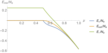
In Fig. 1 we show a plot of the energy for the coherent state and SACS approximations to the ground and first excited state energy for $N_{a}=2$ atoms. We observe that the even SACS state gives an energy below that of the coherent state approximation. The odd SACS state corresponds to the estimation of the energy of the first-excited state. We note that all the SACS estimations approach the coherent one as the intensity of the interaction grows. When the number of particles is larger, the form of the SACS energies approximates the coherent state result; even for $N_{a}=10$ they are very difficult to distinguish.

Figure 1: (Colour online) Ground state energy comparison for the coherent state (orange) and SACS approximations. We consider $N_{a}=2$ atoms, $\Omega=\omega_{2}=\omega_{3}=1$, and $\omega_{1}=0$. We use the variable $\mu$ to denote the intensity of the dipolar interactions. The expectation value for the even and odd SACS states are the lowest (blue) and the highest (green) curves, respectively.

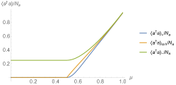
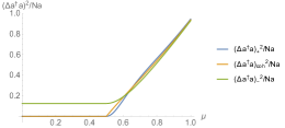
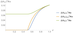
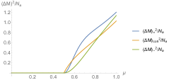
We can calculate also the expectation values of other observables of the system. In Fig. 2 (left) we show a plot of the expectation value of the number of photons per atom vs. the intensity of the dipole interaction for the coherent state and SACS state approximations to the ground state, for $N_{a}=2$ atoms. As before, they all converge when $N_{a}$ grows. In Fig. 2 (right) we also show the behaviour of the squared fluctuation in the number of photons per atom.

Figure 2: (Colour online) Expectation value (left) and squared fluctuation (right) of the number of photons per atom, for the coherent state and SACS approximations, with $N_{a}=2$ atoms. $\mu$ denotes the intensity of the dipolar interactions.

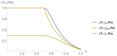
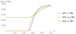
In Figs. 3-4 we present the expectation values for the number of atoms in level $i$, with $i=1,2$, normalised by the number of atoms, and their corresponding fluctuations, respectively, using $N_{a}=2$ atoms. The expectation value for the odd SACS is the lowest of the curves. This behaviour is to be expected because for the odd SACS we have contribution of atoms in the excited states, which diminishes the number of atoms in the lowest level. Exactly the opposite happens for the expectation values of the occupation of the excited levels, as the left side of figure 4 shows. In the right side of figure 3 we show the squared fluctuation for the occupation of the lowest atomic level. The squared fluctuation for the coherent and even SACS states is zero in the normal regime $\mu\leq 0.5$, as is to be expected; then in the collective regime they increase and separate, with the value for the coherent state growing faster. In the normal region the value of the squared fluctuation for the odd SACS is greater, as it also should be. For larger $\mu$ the coherent state fluctuation seems to be the average of the SACS ones. When the intensity of the interaction increases the curves tend to the same value. The behaviour for the fluctuation of the occupancy of the other atomic levels is similar. The squared fluctuation per atom for the coherent and even SACS states is shown for level $i=2$ in Fig. 4 (right). We see that it is zero in the normal regime $\mu\leq 0.5$, for the even SACS and the coherent states. In the normal region the value of the squared fluctuation per atom for the odd SACS state is again greater. The asympotic behaviour is the same as for $i=1$. Because the behaviour for the fluctuation of the occupancy levels $i=2,\,3$ is similar, the latter is not shown.

Figure 3: (Colour online) Comparison of the expectation value of the number atoms in the lowest energy level $i=1$ per atom for the coherent state and SACS approximations (left) and squared fluctuation of the atomic population in energy level $i=1$ per atom for the coherent state and SACS approximations. We considered $N_{a}=2$ atoms, and $\mu$ denotes the intensity of the dipolar interactions.

Figure 4: (Colour online) Comparison of the expectation value of the number atoms in the middle energy level $i=2$ per atom (left), and their corresponding squared fluctuations (right), for the coherent state and SACS approximations. We considered $N_{a}=2$ atoms, and $\mu$ denotes the intensity of the dipolar interactions.

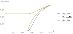
In fact there is a simple relation between the expectation values for levels $i=2,\,3$ and the expectation value of the lowest level $i=1$:

$$\langle\mathbf{A}_{22}\rangle=N_{a}\,\left(1-\frac{1}{N_{a}}\langle\mathbf{A}_{11}\rangle\right)\,\cos^{2}\theta\ ,\quad\langle\mathbf{A}_{33}\rangle=N_{a}\,\left(1-\frac{1}{N_{a}}\langle\mathbf{A}_{11}\rangle\right)\,\sin^{2}\theta\ .$$ (39)

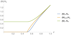
The expectation value of the number of excitations $\mathbf{M}$ for our approximations to the ground and first excited states are shown in Fig. 5 (left). The behaviour is similar to the one exhibited for the expectation value of the number of photons or the occupancy of the upper atomic levels. The expectation value per atom for the coherent and even SACS states is zero in the normal regime, $\mu\leq 0.5$, then in the collective regime they increase and separate with the value for the coherent state growing faster. When the intensity of the interaction increases all the curves tend to the same value. Fig. 5 (right) shows the value of the fluctuations in the total number of excitations for the different approximations. While the even and coherent estimations are the same for the normal regime, we observe that their values are very different in the collective regime.

Figure 5: (Colour online) Expectation value of the number of excitations $\mathbf{M}$ (left) and its corresponding squared fluctuation (right). We considered $N_{a}=2$ atoms, and $\Omega=\omega_{2}=\omega_{3}=1$ and $\omega_{1}=0$. The expectation value per atom for the coherent and even SACS states is zero in the normal regime, $\mu\leq 0.5$. In the collective regime they increase and separate, with the value for the coherent state growing faster.

To determine the statistical behaviour of the total number of excitations $\mathbf{M}$ we define the analogous of the Mandel parameter as

$$Q_{\mathbf{M}}:=\frac{(\Delta\mathbf{M})^{2}}{\langle\mathbf{M}\rangle}-1\ .$$ (40)

In Fig. 6 we show this Mandel parameter. In the normal regime the behaviour of the three approximations is very different. For the even SACS state approximation the value is 1, i.e., the behaviour is superpoissonian, and it starts to decrease at the phase transition $\mu=0.5$ until it crosses to negative values at $\mu\approx 0.54$, becoming a subpoissonian distribution. The odd SACS state approximation has value -1 for the normal regime, i.e., it is subpoissonian, and starts to grow at the critical point, never crossing to positive values, reaching the value of the even SACS state approximation at $\mu\approx 0.56$. After this point they tend asymptotically to zero from negative values of $Q$.

Figure 6: Analogous $Q$ Mandel parameter for the number of excitations $\mathbf{M}$, with $N_{a}=2$ atoms. We observe that in the normal regime the behaviour of the three approximations is very different. For the even SACS state approximation we have the value 1, where we can say that the behaviour is superpoissonian, and it starts to decrease at the phase transition ($\mu=0.5$) until it crosses to negative values at $\mu\approx 0.54$, becoming subpoissonian. The odd SACS state approximation starts at -1 for the normal regime and starts to grow at the critical point, i.e., it is subpoissonian, and then grows until it reaches the value of the even SACS approximation at $\mu\approx 0.56$. After this point they tend asymptotically to zero from negative values of $Q$.

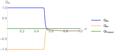
In contrarst, the coherent state approximation gives a poissonian distribution throughout. The SACS state estimation for the photon number distribution function is different than for the coherent state case because in the latter we have components in the states with an even and odd number of excitations. Using Eq. (33) and substituting the minima given in section 4, one gets, for the $V$-configuration in the double-resonance condition

$${\cal P}_{\pm}(\nu)=\left\{\begin{array}[]{cl}\frac{\overline{\nu}^{\nu}}{\nu!}\,\frac{(2\mu)^{N_{a}}\pm(-1)^{\nu}(2\mu)^{-N_{a}}}{(2\mu)^{N_{a}}\,\exp(\overline{\nu})\pm(2\mu)^{-N_{a}}\,\exp(-\overline{\nu})}&,\ \mu^{2}-\frac{1}{4}\geq 0\ ;\\[5.16663pt] \frac{1}{2}(1\pm 1)\,\delta_{\nu\,0}+\frac{1}{4}(1\mp 1)(\delta_{\nu\,0}+\delta_{\nu\,1})&,\ \mu^{2}-\frac{1}{4}\leq 0\ ,\end{array}\right.$$ (41)

where we have defined

$$\overline{\nu}:=N_{a}\frac{\left(\mu^{2}-\frac{1}{4}\right)\left(\mu^{2}+\frac{1}{4}\right)}{\mu^{2}}\ .$$

For comparison, we write the expression for the normal coherent state:

$${\cal P}_{coh}(\nu)=\left\{\begin{array}[]{cl}\frac{\overline{\nu}^{\nu}}{\nu!}\,\exp(-\overline{\nu})&,\ \mu^{2}-\frac{1}{4}\geq 0\ ;\\[3.44444pt] \delta_{\nu\,0}&,\ \mu^{2}-\frac{1}{4}\leq 0\ .\end{array}\right.$$ (42)

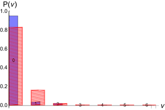
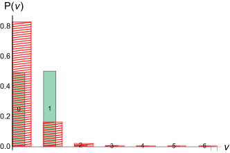
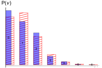
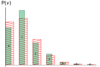
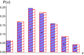
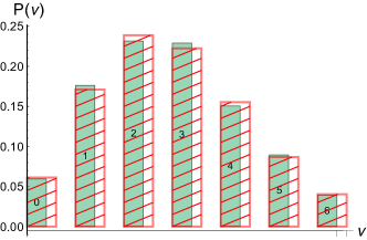
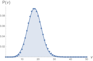
Fig. 7 compares the behaviour of the photon number probability distribution for the coherent state with the even (left) and odd (right) SACS states. As the coherent state contains both, the even and odd number of excitations, this comparison is valid. We can see that the largest difference occurs as we approach $\mu=0.5$, the phase transition from the normal regime to the collective one. For large values of $\mu$ all the distributions are practically the same. They fit a gaussian distribution centered around $\overline{\nu}=17.74$ with standard deviation $\sigma=4.23$, as shown in Fig. 8, where $N_{a}=2$ atoms, and $\mu=3$.

Figure 7: Comparison between the probability distribution of the number of photons $\nu$ for the even (left) and odd (right) SACS states (solid bars) and the coherent state (hatched bars) approximation, in different regions of the dipole interaction parameter space. We considered $N_{a}=2$ atoms. The plots correspond to dipolar intensities $\mu=0.55,\,0.8,\,1.2$, from top to bottom. We can appreciate that both distributions differ more as we approach the phase transition, which occurs at $\mu=0.5$. For greater values of $\mu$ the distributions are practically indistinguishable.

Figure 8: For large values of the dipole interaction parameter $\mu$, all the photon distributions (dots) are practically equal. They approach a normal distribution (solid curve) centered around $\overline{\nu}=17.74$ and standard deviation $\sigma=4.23$. We considered $N_{a}=2$ atoms and $\mu=3$.

In the coherent state approximation to the ground state we have always a separable state. Using the SACS states approximation we have entanglement between the atomic and field parts of the system.

To calculate the entanglement we write down the density matrix corresponding to the state in Eq. (33) and the trace over the electromagnetic part of the system to obtain the reduced density operator of the atomic part. We obtain

$$\left(\mathbf{\rho}^{\pm}_{M}\right)_{n_{2}n_{3},n_{2}^{\prime}n_{3}^{\prime}}=\frac{N_{a}!\ \gamma_{2}^{n_{2}}\,\gamma_{2}^{\ast\ n_{2}^{\prime}}\,\gamma_{3}^{n_{3}}\,\gamma_{3}^{\ast\ n_{3}^{\prime}}}{\sqrt{(N_{a}-n_{2}-n_{3})!\,n_{2}!\,n_{3}!\,(N_{a}-n_{2}^{\prime}-n_{3}^{\prime})!\,n_{2}^{\prime}!\,n_{3}^{\prime}!}}\,$$

$$\quad\times\frac{\Big{[}1+(-1)^{\lambda_{2}(n_{2}+n_{2}^{\prime})+\lambda_{3}(n_{3}+n_{3}^{\prime})}\Big{]}\Big{[}\exp(\left|\alpha\right|^{2})\pm(-1)^{\lambda_{2}n_{2}+\lambda_{3}n_{3}}\exp(-\left|\alpha\right|^{2})\Big{]}}{\Big{[}2\,\left(\exp(\left|\alpha\right|^{2})\,(\gamma^{\ast}\cdot\gamma)^{N_{a}}\pm\exp(-\left|\alpha\right|^{2})\,(\gamma^{\ast}\cdot\tilde{\gamma})^{N_{a}}\right)\Big{]}}\ .$$ (43)

The linear entropy, or purity, which gives a good measure of the entanglement, is defined as $S_{L}=1-\tr(\mathbf{\rho}^{\pm}_{M})^{2}$. Evaluating the previous expression at the minima one gets

$$S^{{}^{\pm}}_{L}=\frac{\left(1-e^{\frac{N_{a}(16\mu^{4}-1)}{4\mu^{2}}}\right)\left(1-(2\mu)^{4N_{a}}\right)}{2\left(1\pm(2\mu)^{2N_{a}}e^{\frac{N_{a}(8\mu^{4}-1)}{4\mu^{2}}}\right)^{2}}\ .$$ (44)

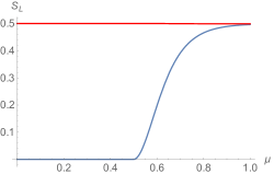
In Fig. 9 we show this quantity for the SACS even and odd approximations. We must emphasize that for the coherent state approximation the result is zero. In contrast, $S^{-}_{L}$ has constant value of $1/2$ for any value of coupling parameter $\mu$. For large values of $\mu$ or the number of particles one has $S^{\pm}_{L}=1/2$.

Figure 9: (Colour online) Linear entropy for the even and odd SACS approximations to the ground and first-excited states. We considered $N_{a}=2$ atoms. The upper curve (red) corresponds to the odd SACS state.

7 Conclusions

The symmetries of the full Hamiltonian (not using the RWA approximation) which describes the dipolar interaction of three-level atoms with a one-mode radiation field lead to a parity conservation in the total excitation number. By using as trial states a combination of coherent states which preserve this symmetry, we obtain a better approximation for the ground state than with the standard coherent states, and a good estimation for the first excited level. This is made explicit by considering the $V$-configuration in the double resonant case, where we calculate the minimum of the energy and the expectation values of many important observables of the system such as the number of photons, the atomic populations, the number of excitations, and their corresponding fluctuations. For the first time, we exhibit analytic expressions for all of these quantities. Also for the first time we obtain an analytic description for the phase diagram in parameter space, which distinguishes the normal and collective regions, and which gives us all the quantum phase transitions of the ground state from one region to the other as we vary the interaction parameters (the matter-field coupling constants) of the model, in functional form.

We also introduce the analogous of the $Q$-Mandel factor for the total number of excitations, which better displays the difference between the modified coherent states and the standard ones. The photon number distribution is also obtained. With the SACS states we are able to write down the reduced density matrix, allowing us to use the tools of quantum information theory to calculate interesting properties of the two lowest states of the system. As an example, we calculate the linear entropy of system to estimate the entanglement between matter and radiation.

Appendix A Unitary transformation of $\mathbf{H}_{R}$

The tranformation of $\mathbf{H}_{R}$ is given by

$$\mathbf{H}_{R}(\theta)=\exp(-i\,\theta\,\mathbf{M})\,\mathbf{H}_{R}\,\exp(i\,\theta\,\mathbf{M})\ .$$ (45)

One can easily find that

$$\frac{d\phantom{\theta}}{d\theta}\,\mathbf{H}_{R}(\theta) = \mathbf{U}(\theta)\,\Big{[}\,\mathbf{M},\,\mathbf{H}_{R}\Big{]}\,\mathbf{U}^{\dagger}(\theta)\ ,$$

$$\frac{d^{2}\phantom{\theta}}{d\theta^{2}}\,\mathbf{H}_{R}(\theta) = \mathbf{U}(\theta)\,\Big{[}\mathbf{M},\,\Big{[}\,\mathbf{M},\,\mathbf{H}_{R}\Big{]}\,\Big{]}\,\mathbf{U}^{\dagger}(\theta)=-4\,\mathbf{H}_{R}(\theta)\ .$$

From these results we deduce that

$$\mathbf{H}_{R}(\theta)=\cos(2\theta)\,\mathbf{H}_{R}+\frac{i}{2}\,\sin(2\theta)\,\Big{[}\,\mathbf{M},\,\mathbf{H}_{R}\,\Big{]}\ .$$ (46)

Therefore the transformation under $\mathbf{U}(\theta)$ leaves $\mathbf{H}_{R}$ invariant if $\theta=\pi+2\pi\,n$, $n\in\mathbb{Z}$, and the states that are invariant under this transformation are given by

$$|\alpha;\,\gamma\}_{\pm}:=\left(\mathbf{1}\pm\exp(i\,\pi\,\mathbf{M})\right)\,|\alpha;\,\gamma\}=|\alpha;\,\gamma\}\pm|\-\alpha;\,\tilde{\gamma}\}\ ,$$ (47)

where $\tilde{\gamma}=(1,\,(-1)^{\lambda_{2}}\gamma_{2},\,(-1)^{\lambda_{3}}\gamma_{3})$.

Appendix B Matrix elements in the SACS basis

In order to calculate the energy surface of the Hamiltonian, with and without the RWA approximation, we need the following matrix elements. For the one-body terms, we have

$${}_{\pm}\{\alpha;\,\gamma|\,\mathbf{A}_{ii}\,|\alpha;\,\gamma\}_{\pm} = 2\,N_{a}\,\left|\gamma_{i}\right|^{2}\,\Big{[}\exp(\left|\alpha\right|^{2})\,(\gamma^{\ast}\cdot\gamma)^{N_{a}-1}$$ (48)

$$\ \pm(-1)^{\lambda_{i}}\,\exp(-\left|\alpha\right|^{2})\,(\gamma^{\ast}\cdot\tilde{\gamma})^{N_{a}-1}\Big{]}\,,$$

$${}_{\pm}\{\alpha\,\gamma|\,\mathbf{a}^{\dagger}\mathbf{a}\,|\alpha\,\gamma\}_{\pm} = 2\,\left|\alpha\right|^{2}\,\Big{[}\,\exp(|\alpha|^{2})\,(\gamma^{\ast}\cdot\gamma)^{N_{a}}\mp\exp(-|\alpha|^{2})\,(\gamma^{\ast}\cdot\tilde{\gamma})^{N_{a}}\Big{]}\ .$$ (49)

For the interaction terms, we have

$${}_{\pm}\{\alpha;\,\gamma|\,\mathbf{A}_{ij}\,\mathbf{a}\,|\alpha;\,\gamma\}_{\pm}=N_{a}\,\alpha\,\gamma_{i}^{\ast}\,\gamma_{j}\,\left(1-(-1)^{\lambda_{i}+\lambda_{j}}\right)$$

$$\qquad\qquad\quad\times\Big{[}\exp(\left|\alpha\right|^{2})\,(\gamma^{\ast}\cdot\gamma)^{N_{a}-1}\pm(-1)^{\lambda_{i}}\,\exp(-\left|\alpha\right|^{2})\,(\gamma^{\ast}\cdot\tilde{\gamma})^{N_{a}-1}\Big{]}\ ,$$ (50)

$${}_{\pm}\{\alpha;\,\gamma|\,(\mathbf{A}_{ij}+\mathbf{A}_{ji})\,(\mathbf{a}+\mathbf{a}^{\dagger})\,|\alpha;\,\gamma\}_{\pm}=N_{a}\,(\alpha+\alpha^{\ast})\,(1-(-1)^{\lambda_{i}+\lambda_{j}})$$

$$\qquad\qquad\qquad\times\Big{[}\,\exp(|\alpha|^{2})\,(\gamma_{i}^{\ast}\,\gamma_{j}+\gamma_{j}^{\ast}\,\gamma_{i})\,(\gamma^{\ast}\cdot\gamma)^{N_{a}-1}$$

$$\qquad\qquad\qquad\pm\exp(-|\alpha|^{2})\,((-1)^{\lambda_{i}}\,\gamma_{i}^{\ast}\,\gamma_{j}+(-1)^{\lambda_{j}}\,\gamma_{j}^{\ast}\,\gamma_{i})\,(\gamma^{\ast}\cdot\tilde{\gamma})^{N_{a}-1}\Big{]}\ .$$ (51)

For the fluctuations in the atomic populations and in the number of photons we need

$${}_{\pm}\{\alpha;\,\gamma|\,\mathbf{A}_{ii}^{2}\,|\alpha;\,\gamma\}_{\pm}=$$

$$\qquad\qquad 2\,N_{a}\,\left|\gamma_{i}\right|^{2}\,\Big{[}\exp(\left|\alpha\right|^{2})\,\left((\gamma^{\ast}\cdot\gamma)^{N_{a}-1}+(N_{a}-1)\,(\gamma^{\ast}\cdot\gamma)^{N_{a}-2}\,\left|\gamma_{i}\right|^{2}\right)$$

$$\qquad\qquad\pm\exp(-\left|\alpha\right|^{2})\,\left((-1)^{\lambda_{i}}\,(\gamma^{\ast}\cdot\tilde{\gamma})^{N_{a}-1}+(N_{a}-1)\,(\gamma^{\ast}\cdot\tilde{\gamma})^{N_{a}-2}\,\left|\gamma_{i}\right|^{2}\right)\Big{]}\ ,$$ (52)

$${}_{\pm}\{\alpha\,\gamma|\,\left(\mathbf{a}^{\dagger}\mathbf{a}\right)^{2}\,|\alpha\,\gamma\}_{\pm} = 2\,|\alpha|^{2}\,\Big{[}\exp(|\alpha|^{2})\,\left(\left|\alpha\right|^{2}+1\right)\,(\gamma^{\ast}\cdot\gamma)^{N_{a}}$$ (53)

$$\qquad\pm\exp(-|\alpha|^{2})\,\left(\left|\alpha\right|^{2}-1\right)\,(\gamma^{\ast}\cdot\tilde{\gamma})^{N_{a}}\Big{]}\ .$$

In order to see the atomic transitions from level $j$ to level $i$, and its quadratic form,

$${}_{\pm}\{\alpha\,\gamma|\,\mathbf{A}_{ij}\,|\alpha\,\gamma\}_{\pm} = N_{a}\,\Big{[}\exp(\left|\alpha\right|^{2})\,\left(\gamma^{\ast}\cdot\gamma\right)^{N_{a}-1}\,\left(\gamma_{i}^{\ast}\,\gamma_{j}+\tilde{\gamma}_{i}^{\ast}\,\tilde{\gamma}_{j}\right)$$ (54)

$$\quad\pm\exp(-\left|\alpha\right|^{2})\,\left(\gamma^{\ast}\cdot\tilde{\gamma}\right)^{N_{a}-1}\,\left(\gamma_{i}^{\ast}\,\tilde{\gamma}_{j}+\tilde{\gamma}_{i}^{\ast}\,\gamma_{j}\right)\Big{]}\ ,$$

$${}_{\pm}\{\alpha\,\gamma|\,\mathbf{A}_{ij}\,\mathbf{A}_{kl}\,|\alpha\,\gamma\}_{\pm} = \Big{[}\exp(\left|\alpha\right|^{2})\,\Big{(}N_{a}\,\delta_{jk}\,(\gamma^{\ast}\cdot\gamma)^{N_{a}-1}\,\left(\gamma_{i}^{\ast}\,\gamma_{l}+\tilde{\gamma}_{i}^{\ast}\,\tilde{\gamma}_{l}\right)$$ (55)

$$+ N_{a}\,(N_{a}-1)\,(\gamma^{\ast}\cdot\gamma)^{N_{a}-2}\,\left(\gamma_{i}^{\ast}\,\gamma_{j}\,\gamma_{k}^{\ast}\,\gamma_{l}+\tilde{\gamma}_{i}^{\ast}\,\tilde{\gamma}_{j}\,\tilde{\gamma}_{k}^{\ast}\,\tilde{\gamma}_{l}\right)\Big{)}$$

$$\pm \exp(-\left|\alpha\right|^{2})\,\Big{(}N_{a}\,\delta_{j\,k}\,(\gamma^{\ast}\cdot\tilde{\gamma})^{N_{a}-1}\,\left(\gamma_{i}^{\ast}\,\tilde{\gamma}_{l}+\tilde{\gamma}_{i}^{\ast}\,\gamma_{l}\right)$$

$$+ N_{a}\,(N_{a}-1)\,(\gamma^{\ast}\cdot\tilde{\gamma})^{N_{a}-2}\,\left(\gamma_{i}^{\ast}\,\tilde{\gamma}_{j}\,\gamma_{k}^{\ast}\,\tilde{\gamma}_{l}+\tilde{\gamma}_{i}^{\ast}\,\gamma_{j}\,\tilde{\gamma}_{k}^{\ast}\,\gamma_{l}\right)\Big{)}\Big{]}\ ;$$

these two expressions allow us to check the first and second order Casimir invariants of $U(3)$.

It is also interesting to evaluate the expectation value of the total number of excitations $\mathbf{M}$, and that of its square in order to obtain the fluctuation and the equivalent to the Mandel parameter:

$${}_{\pm}\{\alpha;\,\gamma|\,\mathbf{M}\,|\alpha;\,\gamma\}_{\pm}$$

$$\qquad=2\,\exp(\left|\alpha\right|^{2})\,(\gamma^{\ast}\cdot\gamma)^{N_{a}-1}\,\Big{[}\left|\alpha\right|^{2}\,(\gamma^{\ast}\cdot\gamma)+N_{a}\sum_{i=2}^{3}\lambda_{i}\,\left|\gamma_{i}\right|^{2}\Big{]}$$

$$\qquad\pm 2\,\exp(-\left|\alpha\right|^{2})\,(\gamma^{\ast}\cdot\tilde{\gamma})^{N_{a}-1}\,\Big{[}-\left|\alpha\right|^{2}\,(\gamma^{\ast}\cdot\tilde{\gamma})+N_{a}\sum_{i=2}^{3}(-1)^{\lambda_{i}}\,\lambda_{i}\,\left|\gamma_{i}\right|^{2}\Big{]}\ ,$$ (56)

$${}_{\pm}\{\alpha;\,\gamma|\,\mathbf{M}^{2}\,|\alpha;\,\gamma\}_{\pm}=2\,\left|\alpha\right|^{2}\,\Big{[}\exp(\left|\alpha\right|^{2})\,\left(\left|\alpha\right|^{2}+1\right)(\gamma^{\ast}\cdot\gamma)^{N_{a}}$$

$$\quad\qquad\pm\exp(-\left|\alpha\right|^{2})\,\left(\left|\alpha\right|^{2}-1\right)(\gamma^{\ast}\cdot\tilde{\gamma})^{N_{a}}\Big{]}$$

$$\qquad+2\,\lambda_{2}^{2}\,N_{a}\,\left|\gamma_{2}\right|^{2}\Big{[}\exp(\left|\alpha\right|^{2})\,\left((N_{a}-1)\,\left|\gamma_{2}\right|^{2}\,(\gamma^{\ast}\cdot\gamma)^{N_{a}-2}+(\gamma^{\ast}\cdot\gamma)^{N_{a}-1}\right)$$

$$\quad\qquad\pm\exp(-\left|\alpha\right|^{2})\,\left((N_{a}-1)\,\left|\gamma_{2}\right|^{2}\,(\gamma^{\ast}\cdot\tilde{\gamma})^{N_{a}-2}+(-1)^{\lambda_{2}}(\gamma^{\ast}\cdot\tilde{\gamma})^{N_{a}-1}\right)\Big{]}$$

$$\qquad+2\,\lambda_{3}^{2}\,N_{a}\,\left|\gamma_{3}\right|^{2}\Big{[}\exp(\left|\alpha\right|^{2})\,\left((N_{a}-1)\,\left|\gamma_{3}\right|^{2}\,(\gamma^{\ast}\cdot\gamma)^{N_{a}-2}+(\gamma^{\ast}\cdot\gamma)^{N_{a}-1}\right)$$

$$\quad\qquad\pm\exp(-\left|\alpha\right|^{2})\,\left((N_{a}-1)\,\left|\gamma_{3}\right|^{2}\,(\gamma^{\ast}\cdot\tilde{\gamma})^{N_{a}-2}+(-1)^{\lambda_{3}}(\gamma^{\ast}\cdot\tilde{\gamma})^{N_{a}-1}\right)\Big{]}$$

$$\qquad+4\,N_{a}\,\lambda_{2}\,\left|\alpha\right|^{2}\,\left|\gamma_{2}\right|^{2}\Big{[}\exp(\left|\alpha\right|^{2})\,(\gamma^{\ast}\cdot\gamma)^{N_{a}-1}\mp(-1)^{\lambda_{2}}\exp(-\left|\alpha\right|^{2})\,(\gamma^{\ast}\cdot\tilde{\gamma})^{N_{a}-1}\Big{]}$$

$$\qquad+4\,N_{a}\,\lambda_{3}\,\left|\alpha\right|^{2}\,\left|\gamma_{2}\right|^{2}\Big{[}\exp(\left|\alpha\right|^{2})\,(\gamma^{\ast}\cdot\gamma)^{N_{a}-1}\mp(-1)^{\lambda_{3}}\exp(-\left|\alpha\right|^{2})\,(\gamma^{\ast}\cdot\tilde{\gamma})^{N_{a}-1}\Big{]}$$

$$\qquad+4\,N_{a}(N_{a}-1)\,\lambda_{2}\,\lambda_{3}\,\left|\gamma_{2}\right|^{2}\,\left|\gamma_{3}\right|^{2}\,\Big{[}\exp(\left|\alpha\right|^{2})\,(\gamma^{\ast}\cdot\gamma)^{N_{a}-2}$$

$$\quad\qquad\mp(-1)^{\lambda_{2}+\lambda_{3}}\exp(-\left|\alpha\right|^{2})\,(\gamma^{\ast}\cdot\tilde{\gamma})^{N_{a}-2}\Big{]}\ .$$ (57)

References

- [1] Garraway B M, 2011 Phil. Trans. R. Soc. A 369, 1137, and references therein.
- [2] Nahmad-Achar E, Castaños O, López-Peña R and Hirsch J G, 2013 Phys. Scr. 87, 038114.
- [3] Lanyon B, Weinhold T, Langford N, O’Brien J, Resch K, Gilchrist A, and White A, 2008 Phys. Rev. Lett. 100, 060504.
- [4] Imre S and Gyongyosi L, 2013 Advanced Quantum Communications: An Engineering Approach, (Hoboken, New Jersey: John Wiley & Sons).
- [5] Yoo H-I and Eberly J H, 1985 Phys. Rep. 118, 239.
- [6] Li X S and Peng Y N, 1985 Phys. Rev. A 32, 1501.
- [7] Peng J-S, Li G-X and Zhou P, 1992 Phys. Rev. A 46, 1516.
- [8] Aliskenderov E I, Ho Trung Dung and Shumovsky A S, 1991 Quantum Opt. 3, 241.
- [9] Ho Trung Dung, Tanas R and Shumovsky A S, 1991 Quantum Opt. 3, 255.
- [10] Klimov A B, Sánchez-Soto L L, Delgado J and Yustas E C, 2003 Phys. Rev. A 67, 013803.
- [11] Hayn M, Emary C and Brandes T, 2011 Phys. Rev. A 84, 053856.
- [12] Abdel-Wahab N H, 2007 Phys. Scr. 76, 244.
- [13] Cordero S, López-Peña R, Castaños O and Nahmad-Achar E, 2013 Phys. Rev. A 87, 023805.
- [14] Cordero S, Castaños O, López-Peña R and Nahmad-Achar E, 2013 Jour. Phys. A: Math. Theor. 46, 505302.
- [15] Arecchi F T, Courtens E, Gilmore R and Thomas H, 1972 Phys. Rev. A 6, 2211; Gilmore R, Bowden C M and Narducci L M, 1975 Phys. Rev. A 12, 1019. Ginocchio J and Kirson M W, 1980 Phys. Rev. Letters 44, 1744; Nucl. Phys. A 350, 31. Iachello I, and Arima A, The Interacting Boson Model, 1987 (New York, NY: Cambridge University Press).