Abstract

A density estimation method in a Bayesian nonparametric framework is presented when recorded data are not coming directly from the distribution of interest, but from a length biased version. From a Bayesian perspective, efforts to computationally evaluate posterior quantities conditionally on length biased data were hindered by the inability to circumvent the problem of a normalizing constant. In this paper we present a novel Bayesian nonparametric approach to the length bias sampling problem which circumvents the issue of the normalizing constant. Numerical illustrations as well as a real data example are presented and the estimator is compared against its frequentist counterpart, the kernel density estimator for indirect data of Jones (1991).

Keywords: Bayesian nonparametric inference; Length biased sampling; Metropolis algorithm.

1 Introduction

Let $f(x;\theta)$, with $\theta\in\Theta$ being an unknown parameter, be a family of density functions. Sampling under selection bias involves observations being drawn not from $f(x;\theta)$ directly, but rather from a distribution which is a biased version of $f(x;\theta)$, given by the density function

$$g(y;\theta)=\frac{w(y)\,f(y;\theta)}{\int_{0}^{\infty}w(x)\,f(x;\theta)\,dx}.$$

where the $w(x)>0$ is the weight function. We observe a sample $(Y_{1},\ldots,Y_{n})$, independently taken from $g(\cdot)$. In particular, when the weight function is linear; i.e. $w(y)=y$, the samples are known as length biased.

There are many situations where weighted data arise; for example, in survival analysis (Asgharian et al., 2002); quality control problems for estimating fiber length distributions (Cox, 1969); models with clustered or over–dispersed data (Efron, 1986); visibility bias in aerial data; sampling from queues or telephone networks. For further examples of length biased sampling see, for example, Patil and Rao (1978) and Patil (2002).

In the nonparametric setting $f(x;\theta)$ is replaced by the more general $f(x)$, so the likelihood function for $n$ data points becomes,

$$l(f)=\prod_{i=1}^{n}\frac{y_{i}\,f(y_{i})}{\int_{0}^{\infty}x\,f(x)\,dx}.$$

A classical nonparametric maximum likelihood estimator (NPMLE) for $F$ (the disribution function corresponding to $f$) exists for this problem and is discrete, with atoms located at the observed data points. In particular, Vardi (1982) finds an explicit form for the estimator in the presence of two independent samples, one from $f$ and the other from the length biased density $g$.

Our work focuses on length biased sampling and from the Bayesian nonparametric setting we work in, the aim is to obtain a density estimator for $f$. There has been no work done on this problem in the Bayesian nonparametric framework due to the issue of the intractable likelihood function, particularly when $f$ is modeled nonparametrically using, for example, the mixture of Dirichlet process (MDP) model; see Lo (1984) and Escobar and West (1995). While some ideas do exist on how to deal with intractable normalizing constants; see Murray et al. (2006); Tokdar, (2007); Adams et al. (2009); and Walker, (2011), these ideas fail here for two reasons: the infinite dimensional model and the unbounded $w(y)=y$ when the space of observations is the positive reals.

We by-pass the intractable normalizing constant by modeling $g$ nonparametrically. We argue that modeling $f$ or $g$ nonparametrically is providing the same flexibility to either; i.e. modeling $f(y)$ nonparametrically and defining $g(y)\propto y\,f(y)$ is essentially equivalent to modeling $g(y)$ nonparametrically and defining $f(y)\propto y^{-1}g(y)$. We adopt the latter style, obtain samples from the predictive density of $g$ and then “convert” these samples from $g$ into samples from $f$, which forms the basis of the density estimator of $f$.

The layout of the paper is as follows: In Section 2 we provide supporting theory for the model idea which avoids the need to deal with the intractable likelihood function. Section 3 describes the model and the MCMC algorithm for estimating it and Section 4 describes some numerical illustrations. In Section 5 are the concluding remarks and in Section 6 asymptotic results are provided.

2 Supporting theory and methodology

Our aim is to avoid computing the intractable normalizing constant. The strategy for that would be to model the density $g(y)$ directly and then make inference about $f(x)$ by exploiting the fact that

$$g(y)\propto y\,f(y).$$

In the parametric case if a family $f(x;\theta)$ is known then so is $g(y;\theta)$, except its normalizing constant may not be tractable. There is a reluctance to avoid the problem of the normalizing constant in the parametric case by modeling the data directly with a tractable $g(y;\theta)$ since the incorrect model would be employed. However, in the nonparametric setting it is not regarded as relevant whether one models $f(\cdot)$ or $g(\cdot)$ directly. A clear motivation to model $g(\cdot)$ directly is that this is where the data are coming from.

For a general weight function $w$, an essential condition to model $F$ through $G$ ($F$ and $G$ denote the corresponding distribution functions of $f$ and $g$, respectively) is the finiteness of $\int_{0}^{\infty}w(x)^{-1}\,g(x)\,dx$. This, through invertibility, enables us to reconstruct $F$ from $G$ and occurs when $F$ is absolutely continuous with respect to $G$, with the Radon-Nikodym derivative being proportional to $w(x)^{-1}$.

For absolute continuity to hold we need that $w(x)>0$ in the support of $F$ ie $F(x:w(x)=0)=0$. In the length biased case examined here $w(x)=x$ and the densities have support on the positive real line, so this condition is automatically satisfied. A case, for instance, when this does not hold and invertibility fails is in a truncated model where $w(x)=1(x\in B)$, $B$ is a Borel set and $F$ is a distribution which could be positive outside of $B$.

A Bayesian model is thus constructed by assigning an appropriate nonparametric prior distribution to $g$, provided that

$$\int_{0}^{\infty}y^{-1}\,g(y)\,dy<\infty.$$

This in turn specifies a prior for $f$.

The question that now arises is how the posterior structures obtained after modelling $g$ directly can be converted to posterior structures from $f$. The first step in this process would be to devise a method to convert a biased sample from a density $g$ to one from its debiased version $f$. This algorithm is then incorporated to our model building process so that posterior inference becomes possible.

Specifically, assume that a sample $y_{1},\ldots,y_{N}$, comes from a biased density $g$. This can be converted into a sample from $f(x)\propto x^{-1}g(x)$ using a Metropolis–Hastings algorithm. If we denote the current sample from $f(x)$ as $x_{j}$, then

$$x_{j+1}=y_{j+1}\quad\mbox{with probability}\quad\min\left\{1,\frac{x_{j}}{y_{j+1}}\right\},$$

otherwise $x_{j+1}=x_{j}$. Here, we have the transition density for this process as

$$p(x_{j+1}|x_{j})=\min\left\{1,\frac{x_{j}}{x_{j+1}}\right\}g(x_{j+1})+\left\{1-r(x_{j})\right\}{\bf 1}(x_{j+1}=x_{j}),$$

where

$$r(x)=\int\min\left\{1,\frac{x}{x^{*}}\right\}g(x^{*})\,dx^{*}.$$

This transition density satisfies detailed balance with respect to $f(x)$ since

$$p(x_{j+1}|x_{j})\,x_{j}^{-1}g(x_{j})=p(x_{j}|x_{j+1})\,x_{j+1}^{-1}g(x_{j+1})$$

and thus the transition density has stationary density given by $f(x)$.

This algorithm was first tested on a toy example, i.e. $g(y)$ is Ga$(y|2,1)$ so that $f(x)$ is Ga$(x|1,1)$. A sample of $N=10,000$ of the $(y_{j})$ was taken independently from the $g(\cdot)$ and the Metropolis algorithm run to generate the $(x_{j})$, starting with $x_{0}=1$. Sample values for the sequence of $(x_{j})$ yield

$$N^{-1}\sum_{j=1}^{N}x_{j}=0.981\quad\mbox{and}\quad N^{-1}\sum_{j=1}^{N}x_{j}^{2}=1.994,$$

which are compatible outcomes with the $(x_{j})$ sample coming from $f(x)$. A similar example will be elaborated on in the numerical illustration section.

Applying this idea to our model would amount to turning a sample from the biased posterior predictive density to an unbiased one using a MH step. An outline of the inferential methodology is now described.

1. Once data $(y_{1},\ldots,y_{n})$ from a biased distribution $g$ become avalaible a model for $g$ is assumed and a nonparametric prior is assigned.

2. Using MCMC methods, after a sensible burn-in period, at each iteration, posterior values of the random measure $\Pi(dg|y_{1},\ldots,y_{n})$ and the relevant parameters are obtained. Subsequently, conditionally on those values, a sequence $\{y_{n+1}^{(l)}\},\;l=1,2,\ldots$, from the posterior predictive density $g(y|y_{1},\ldots,y_{n})$ is generated.

3. The $\{y_{n+1}^{(l)}\}$ will then form a sequence of proposal values of a Metropolis-Hastings chain with stationary density the debiased version of the posterior predictive, i.e. $\propto y^{-1}g(y|y_{1},\ldots,y_{n})$. Specifically, at the $l$-th iteration of the algorithm applying a rejection criterion a value $x_{n+1}^{(l)}$ is generated such that $x_{n+1}^{(l)}=y_{n+1}^{(l)}$ with probability $\min\left\{1,x_{n+1}^{(l-1)}/y_{n+1}^{(l)}\right\}$, otherwise $x_{n+1}^{(l)}=x_{n+1}^{(l-1)}$.

4. These $\{x_{n+1}^{(l)}\}$ values form a sample from the posterior predictive of $f$.

3 The model and inference

We want the model for $g(y)$ to have large support and the standard Bayesian nonparametric idea for achieving this is based on infinite mixture models (Lo, 1984) of the type

$$g_{\mathbb{P}}(y)=\int k(y;\theta)\,{\mathbb{P}}(d\theta)$$

where ${\mathbb{P}}$ is a discrete probability measure and $k(y;\theta)$ is a density on $(0,\infty)$ for all $\theta$. Since we require $g(y)$ to be such that

$$\int_{0}^{\infty}y^{-1}\,g_{\mathbb{P}}(y)\,dy<\infty$$

or, equivalently, for a kernel $k(y;\theta)$

$$\int_{0}^{\infty}\,y^{-1}k(y;\theta)dy<\infty$$

we find it most appropriate to take the kernel to be a log–normal distribution. So, assuming a constant precision parameter $\lambda$ for each component, we have

$$g_{\lambda,{\mathbb{P}}\,}(y)=\int_{\mathbb{R}}\mbox{LN}(y|\,\mu,\lambda^{-1})\,{\mathbb{P}}(d\mu)$$ (1)

where ${\mathbb{P}}$ is a discrete random probability measure defined in ${\mathbb{R}}$ and ${\mathbb{P}}\sim{\rm DP}(c,P_{0})$, where ${\rm DP}(c,P_{0})$ denotes the Dirichlet process (Ferguson, 1973) with precision parameter $c>0$ and base measure $P_{0}$. Interpreting the parameters, we have that ${\rm E}({\mathbb{P}(A)})=P_{0}(A)$, and

$${\rm Var}({\mathbb{P}}(A))={P_{0}(A)(1-P_{0}(A))\over c+1}$$

for appropriate sets $A$.

This Dirichlet process mixture model implies the hierarchical model for $y=(y_{1},\ldots,y_{n})$: For $1\leq i\leq n$

$$y_{i}|\,\mu_{i},\lambda\,\stackrel{{\scriptstyle\rm ind}}{{\sim}}\,\mbox{LN}(\mu_{i},\lambda^{-1})$$

$$\mu_{i}|\,{\mathbb{P}}\,\stackrel{{\scriptstyle\rm i.i.d.}}{{\sim}}\,{\mathbb{P}}$$

$${\mathbb{P}}|\,c,P_{0}\,\sim\,{\rm DP}(c,P_{0})$$

To complete the model we choose $\lambda\sim$ Ga$(a,b)$ and for the base measure, $P_{0}$ is ${\rm N}(0,s^{-1})$.

A useful representation of the Dirichlet process, introduced by Sethuraman and Tiwari (1982) and Sethuraman (1994), is the stick–breaking constructive representation given by

$${\mathbb{P}}\,=\,\sum_{j=1}^{\infty}w_{j}\,\delta_{\mu_{j}}$$

where the $(\mu_{j})$ are i.i.d. from $P_{0}$, i.e. ${\rm N}(0,s^{-1})$. The $(w_{j})$ are constructed via a stick–breaking process; so that $w_{1}=v_{1}$ and, for $j>1$,

$$w_{j}=v_{j}\prod_{l<j}(1-v_{l})$$ (2)

where the $(v_{j})$ are i.i.d. from the beta$(1,c)$ distribution, for some $c>0$, and $\sum_{j=1}^{\infty}w_{j}=1$ almost surely. Let $w=(w_{j})_{j=1}^{\infty}$ and $\mu=(\mu_{j})_{j=1}^{\infty}$; then we can then write

$$g(y_{i}|\mu,w,\lambda)=\sum_{j=1}^{\infty}w_{j}\,\mbox{LN}\left(y_{i}|\mu_{j},\lambda^{-1}\right)$$ (3)

This is a standard Bayesian nonparametric model. The MCMC algorithm is implemented using latent variable techniques, despite the infinite dimensional model. The basis of this sampler is in Walker (2007) and Kalli et al. (2011).

For $1\leq i\leq n$ we introduce latent variables $u_{i}$ which make the sum finite. The $u_{i}$ augmented density then becomes,

$$\begin{split}g(y_{i},u_{i}|\,w,\mu,\lambda)\,=\,\sum_{j=1}^{\infty}{\bf 1}(u_{i}<w_{j})\mbox{LN}\left(y_{i}|\mu_{j},\lambda^{-1}\right)\,=\\ =\sum_{j\in A_{w}(u_{i})}\mbox{LN}\left(y_{i}|\mu_{j},\lambda^{-1}\right)\end{split}$$ (4)

This has a finite representation and $A_{w}(u_{i})$ denotes the almost surely finite $u_{i}$ slice set $\{j:u_{i}<w_{j}\}$.

Now we introduce latent variables $\{d_{1},\ldots,d_{n}\}$ which allocate the component that $\{y_{1},\ldots,y_{n}\}$ are sampled from. Conditionally on the weights $w$ these are sampled independently with $P(d_{i}=j|w)=w_{j}$. Hence, we consider the $(u_{i},d_{i})$ augmented random density

$$g(y_{i},u_{i},d_{i}|\,w,\mu,\lambda)\,=\,{\bf 1}(u_{i}<w_{d_{i}})\mbox{LN}\left(y_{i}|\mu_{d_{i}},\lambda^{-1}\right)$$

Therefore, the complete data likelihood based on a sample of size $n$ is seen to be

$$l(y,u,d|\,w,\mu,\lambda)\,=\,\prod_{i=1}^{n}{\bf 1}(u_{i}<w_{d_{i}})\mbox{LN}\left(y_{i}|\mu_{d_{i}},\lambda^{-1}\right)$$

This will form the basis of our Gibbs sampler. At each iteration we sample from the associated full conditional densities of the following variables:

$$(v_{j},\mu_{j}),\;j=1,\ldots,N;\;\lambda;\;(d_{i},u_{i}),\;i=1\ldots n$$

where $N$ is a random variable, such that $\cup_{i=1}^{n}A_{w}(u_{i})\subseteq\{1,\ldots,N\}$, and $N<\infty$ almost surely.

These distributions are, by now, quite standard so we proceed directly to the last two steps of the algorithm.

The upshot is that after a sensible burn–in time period given the current selection of parameters, at each iteration, we can sample values $y_{n+1}$ from the posterior predictive density $g(y|y_{1},\ldots,y_{n})$ and subsequently, using a Metropolis step, draw a $z$ value from its debiased version $f(\cdot|y_{1},\ldots,y_{n})$.

• Once stationarity is reached then at each iteration we have points generated by the posterior measure of the variables. These points are represented by

  $$\{(v_{j}^{*},\mu_{j}^{*}),\;j=1,2\ldots\;;\lambda^{*};\;(d_{i}^{*},u_{i}^{*}),\;i=1\ldots n;\;\}$$

  Given $\{w_{j}^{*},\mu^{*}_{j},\lambda^{*}\}$ a value $y_{n+1}\,\sim g(y|y_{1},\ldots,y_{n})$ is generated. This is done by sampling a $r$ uniformly in the unit interval and then take $k=1$ if $0<r\leq w^{*}_{1}$ or $k\geq 2$ if

  $$\sum_{i=1}^{k-1}w_{j}^{*}<r\leq\sum_{j=1}^{k}w_{j}^{*}$$

  The appropriate $\mu_{n+1}^{*}=\mu_{k}^{*}$ is then assigned, with probability $w^{*}_{k}$. Even though we have not sampled all the weights, if we “run out” of weights, in essence the indices {1,…,N}, we merely draw a $\mu_{n+1}^{*}$ from ${\rm N}(0,s^{-1})$. Finally, the predictive value $y_{n+1}$ comes from $\mbox{LN}(y|\mu_{n+1}^{*},\lambda^{*})$.

• The Metropolis step for the posterior predictive of $f$: Let $\tilde{x}$ be the state of the chain from the previous Gibbs iteration. Accept the sample $y_{n+1}$, from the $g$-predictive, as coming from the $f$-predictive, that is $z=y_{n+1}$, with probability $\min\{1,\tilde{x}/y_{n+1}\}$; otherwise the chain remains in its current state i.e. $z=\tilde{x}$.

4 Numerical illustrations

We illustrate the model with two simulated data sets and a real data example. In each of the assumed models, for a given realisation $(y_{1},\ldots,y_{n})$, we report on the results and compare them with the following density estimators:

• The classical kernel density estimate given by

  $${\widetilde{g}}_{h}\,(y;\,(y_{1},\ldots,y_{n}))\,\propto\,n^{-1}\,\sum_{j\,=1}^{n}{\rm N}\left(y|\,y_{j},h^{2}\right){\bf 1}(y>0).$$ (5)

• The kernel density estimate for indirect data, see Jones (1991), is given by

  $${\widehat{f}}_{J,h}\,(y;\,(y_{1},\ldots,y_{n}))\,\propto\,n^{-1}{\widehat{\mu}}\,\sum_{j\,=1}^{n}y_{j}^{-1}\,{\rm N}\left(y|\,y_{j},h^{2}\right){\bf 1}(y>0),$$ (6)

  where ${\widehat{\mu}}$ is the harmonic mean of $(y_{1},\ldots,y_{n})$.

Here $h$ is the bandwidth and in all cases an estimate of it has been calculated as the average of the plug–in and solve–the–equation versions of it, (Sheather and Jones $1991$). The Gibbs sampler iterates $60,000$ times with a burn–in period of $10,000$.

4.1 Simulated Data Examples

Here we use non informative prior specifications:

$$\pi(\lambda)\propto 1/\lambda,\quad{\rm and}\quad\mu_{j}\sim{\rm N}(0,0.5^{-1}).$$ (7)

The value of the concentration parameter has been set to $c=1$.

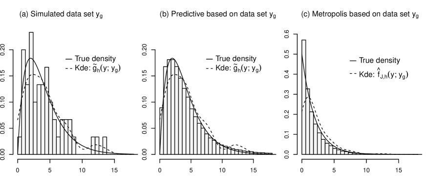
Example 1. The length biased distribution is $g(y)={\rm Ga}(y|\,2,0.5)$ and we simulate $y_{\rm g}=(y_{1},\ldots,y_{n})$ of size $n=50$. The following results are presented Figure 1:

• 1(a): (i) a histogram of the simulated length biased data set $y_{\rm g}$, ii) the true biased density Ga$(2,0.5)$ (the solid line) and iii) the kernel density estimate $\widetilde{g}_{h}(y;y_{\rm g})$ (the dashed line).

• 1(b): (i) a histogram of a sample from the posterior predictive density $g(y_{n+1}|y_{\rm g})$, (ii) the true biased density Ga$(2,0.5)$ (the solid line) and iii) the kernel density estimate $\widetilde{g}_{h}(y;y_{\rm g})$ (the dashed line).

• 1(c): (i) a histogram of the debiased data associated with the application of the Metropolis step, ii) the true debiased density $\exp(0.5)$ (the solid line) and iii) Jones’ kernel density estimate ${\widehat{f}_{J,h}(y;y_{\rm g}})$ (the dashed line).

For both estimators $\widetilde{g}_{h}(y;y_{\rm g})$ and ${\widehat{f}}_{J,h}(y;y_{\rm g})$ the bandwidth parameter is set at $h=1.06$. The average number of clusters ${\cal C}_{g}$ is $4.27$. As it can be seen from the graphs we are hitting the right distributions with the Metropolis step.

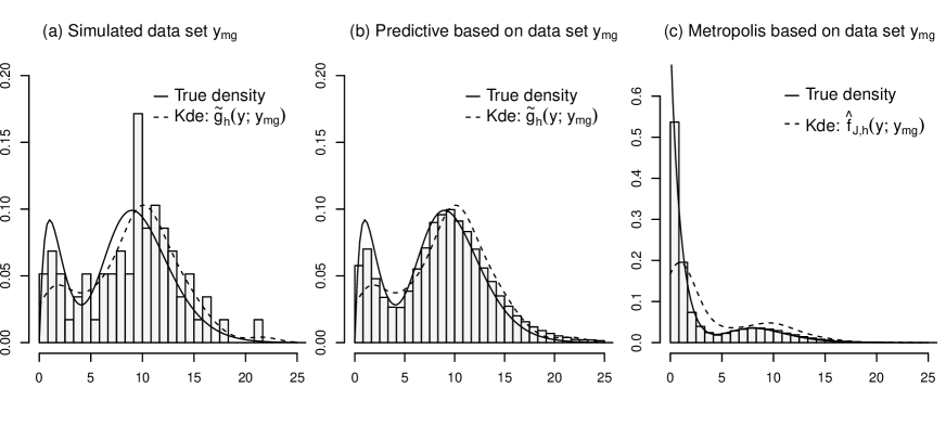
Example 2. Here the length biased distribution is the mixture

$$g(x)=0.25\,{\rm Ga}(x|\,2,1)+0.75\,{\rm Ga}(x|\,10,1)$$

We simulate a sample $y_{\rm mg}=(y_{1},\ldots,y_{n})$ of size $n=70$. Similar results, as in the first example, are shown in Figure $2$, (a)–(c). For both estimators $\widetilde{g}_{h}(y;y_{\rm mg})$ and ${\widehat{f}}_{J,h}(y;y_{\rm mg})$ the bandwidth parameter has been calculated to $h=1.48$. For the average number of clusters, we estimate ${\cal C}_{\rm mg}=5.55$. It is noted that the Metropolis sampler produces samples that are very close to the debiased mixture $f(x)=0.75\,{\rm Ga}(x|\,1,1)+0.25\,{\rm Ga}(x|\,9,1)$ depicted with a solid line in $2$(c).

Figure 1: Data set from Ga$(2,0.5)$ of size $n=50$. In all subfigures the true densities are depicted with a solid line and the kernel density estimates $\tilde{g}_{h}$ and $\hat{f}_{J,h}$ with a dashed line.

Figure 2: Data set from the mixture $0.25\,{\rm Ga}(2,1)+0.75\,{\rm Ga}(10,1)$, $n=70$ . In all subfigures the true densities are depicted with a solid line and the kernel density estimates $\tilde{g}_{h}$ and $\hat{f}_{J}$ with a dashed line.

Figure 3: Data set of size $n=46$ measuring the widths of shrubs. Kernel density estimates $\tilde{g}_{h}$ (classical) and $\hat{f}_{J,h}$ (indirect data) are depicted with dashed lines. Top figures indicate a noninformative prior specificaion while bottom figures an informative one. Such choice reproduces classical estimation results.

Figure 4: (a) the Metropolis acceptance rate running average(MAR–RAV),(b) the predictive running average (P–RAV) and (c) the Metropolis sample running average (M–RAV).

Figure 5: The autocorrelation functions based on the posterior predictive observations. In (a),(b) the gamma and mixture of gammas synthetic data. In c) the width of shrubs real data.

4.2 Real Data Example

The data can be found in Muttlak and McDonald (1990) and consist of $y_{\rm mm}=(y_{1},\ldots,y_{n})$, $n=46$, measurements representing the widths of shrubs obtained by line–transect sampling. In this sampling method the probability of inclusion in the sample is proportional to the width of the shrub making it a case of length biased sampling. A noninformative estimation is shown in Figure $3$ (a)-(c) with the same specifications as in (7) while in $3$(d), 3(e) we perform a highly informative estimation with $\pi(\lambda)={\rm Ga}(\lambda|\,3,0.01)$.

The following results are presented in Figures $3$ and $4$:

• $3$(a), $3$(b): histograms of the length biased data set $y_{\rm mm}$ and of a sample from the posterior predictive $g(y_{n+1}|\,y_{\rm mm})$, respectively . In both subfigures the associated classical estimator $\widetilde{g}_{h}(y;y_{\rm mm})$ is depicted with a dashed line, for $h=0.23$.

• $3$(c): a histogram of the debiased data associated with the Metropolis chain estimator. Jones’ estimator ${\widehat{f}}_{J,h}(y;y_{\rm mm})$ is shown in dashed line, for the same bandwidth value.

• $3$(d), $3$(e): histograms of the posterior predictive and the Metropolis sample, respectively, under the highly informative prior $\pi(\lambda)={\rm Ga}(\lambda|\,3,0.01)$, with superimposed classical density estimators.

• $4$(a): the running acceptance rate of the Metropolis with jump distribution the posterior predictive values from $g(y_{n+1}|\,y_{\rm mm})$ with an estimated value of about $0.62$.

• $4$(b), $4$(c): running averages of the predictive and Metropolis samples respectively.

Finally, in Figure 5 we provide the autocorrelation function as a function of lag, among the values of the posterior predictive sample for the synthetic and real data sets, after a reasonable burn-in period.

4.3 Remarks

• Estimation for the simulated data is nearly perfect and we get the best results for $\pi(\lambda)\propto 1/\lambda$. As it is evident from subfigure $1$(c), for the $\exp(0.5)$, the estimator ${\hat{f}}_{J,h}$ does not properly capture the distributional features near the origin. The same holds true for the ’debiased’ mixture density $0.75\,{\rm Ga}(x|\,1,1)+0.25\,{\rm Ga}(x|\,9,1)$, subfigure $2$(c).

• For the real data set the $1/\lambda$ prior gives again the best results. Such a prior gives the largest average number of clusters among all noninformative specifications that were examined. The debiased $f$ density is close to ${\widehat{f}}_{J,h}$ though not exactly the same. The difference comes from a small area where the biased data have the group of observations $(1.85,1.85,1.86)$ that causes ${\widehat{f}}_{J,h}$ to produce an intense second mode. Excluding these $3$ data points Jones’ estimator ${\widehat{f}}_{J,h}$ becomes identical with ours.

• The highly informative specification $\lambda\sim{\rm Ga}(3,0.01)$ increases the average number of clusters from $4.03$ (noninformative estimation) to about $5.63$, thus the appearance of a second mode between $1.2$ and $2.0$, in $3$(d). From our numerical experiments it seems that ${\widehat{f}}_{J,h}$ is ”data hunting” in the sense that it overestimates data sets and produces spurious modes. Our method performs better as it does not tend to overestimate, and at the same time has better properties near the origin.

• When informative prior specifications are used they increase the average number of realized clusters and the nonparametric estimates tend to look more like Jones’ type estimates. For example choices of $\lambda$ priors like Ga$(\alpha,0.01)$ with $\alpha\geq 2.5$ increase considerably the average number of clusters and our real data estimates in subfigures $3$(d) and 3(e) become nearly identical to ${\widehat{f}}_{J,h}$ .

5 Discussion

In this paper we have described a novel approach to the Bayesian nonparametric modeling of a length bias sampling model. We directly tackle the length bias sampling distribution, from where the data arise, and this technique avoids the impossible situation of the normalizing constant if one decides to model the density of interest directly. This is legitimate modeling since only mild assumptions are made on both densities, so we are free to model $g$ directly and choose an appropriate kernel with the only condition that $\int_{0}^{\infty}x^{-1}k(x,\theta)dx<\infty$.

In a parametric set-up since $f$ is known up to a parameter $\theta$ modeling $g$ directly is not recommended, since to avoid a normalizing constant problem a model for $g$ would not result from the correct family for $f$.

We have also as part of the solution presented a Metropolis step to “turn” the samples from $g(\cdot)$ into samples from $f(\cdot)$. A rejection sampler here would not work as the $1/y$ is unbounded.

The method we have proposed here should also be applicable to an arbitrary weight function $w(y)$, whereby samples are obtained from $g(y)$ and yet interest focuses on the density function $f(y)$, where the connection is provided by

$$g(y)=\frac{w(y)\,f(y)}{\int_{0}^{\infty}w(y)\,f(y)\,dy}.$$

Our estimator, besides being the first Bayesian kernel density estimator for length biased data, it was demonstrated that it performs at least as well and in some cases even better than its frequentist counterpart.

Appendix: Asymptotics

In this section we assume that the posterior predictive sequence $(g_{n})_{n\geq 1}$ is consistent in the sense that $d_{1}(g_{n},g_{0})\rightarrow 0$ a.s. as $n\rightarrow\infty$, where $g_{0}$ is the true density function generating the data and $d_{1}$ denotes the $L_{1}$ distance. This would be a standard result in Bayesian nonparametric consistency involving mixture of Dirichlet process models: see, for example, Lijoi et al. (2005), where sufficient conditions for the $L_{1}$ consistency are given.

The following theorem establishes a similar consistency result for the debiased density.

Theorem. Let $f_{n}(y)\propto y^{-1}g_{n}(y)$ and $f_{0}(y)\propto y^{-1}g_{0}(y)$ denote the sequence of posterior predictive estimates for the debiased density and the true debiased density, respectively. Then, $d_{1}(f_{n},f_{0})\rightarrow 0$ a.s.

Proof. Let

$$g_{n}(y)=\int\mbox{LN}(y|\mu,\sigma^{2})\,dP_{n}(\mu,\sigma^{2})$$

where $P_{n}$ is the posterior expectation of $P$, and for some $P_{0}$ it is that

$$g_{0}(y)=\int\mbox{LN}(y|\mu,\sigma^{2})\,dP_{0}(\mu,\sigma^{2}).$$

The assumption of consistency also implies that $P_{n}$ converges weakly to $P_{0}$ with probability one. This means for any continuous and bounded function $h(\mu,\sigma^{2})$ of $(\mu,\sigma^{2})$ we have the a.s. weak consistency of $P_{n}$ implies

$$\int h(\mu,\sigma^{2})\,dP_{n}(\mu,\sigma^{2})\rightarrow\int h(\mu,\sigma^{2})\,dP_{0}(\mu,\sigma^{2})\quad\mbox{a.s.}$$

and note that

$$\int_{0}^{\infty}y^{-1}\,\mbox{LN}(y|\mu,\sigma^{2})\,dy=\exp\{-\mu+\sigma^{2}/2\}.$$

We now aim to show that these results imply the a.s. $L_{1}$ convergence of $f_{n}(y)$ to $f_{0}(y)$. To this end, if we construct the prior so that for some constants $M$ and $\sigma^{*}$ it is that $\underline{\sigma}<\sigma<\overline{\sigma}$ and $|\mu|<M$, assuming $P_{0}$ puts all the mass on $[-M,+M]\times(\underline{\sigma}^{2},\overline{\sigma}^{2})$, then from the definition of weak convergence we have that, with probability one,

$$\begin{split}c_{n}=\int y^{-1}g_{n}(y)\,dy=\int\exp\{-\mu+\sigma^{2}/2\}\,dP_{n}(\mu,\sigma^{2})\\ \rightarrow c_{0}=\int\exp\{-\mu+\sigma^{2}/2\}\,dP_{0}(\mu,\sigma^{2}).\end{split}$$

Also, with the conditions on $(\mu,\sigma^{2})$, we have

$$h_{y}(\mu,\sigma^{2})=y^{-1}\mbox{LN}(y|\mu,\sigma^{2})$$

is a bounded and continuous function of $(\mu,\sigma^{2})$ for all $y>0$. Hence

$$\begin{split}\int y^{-1}\mbox{LN}(y|\mu,\sigma^{2})\,dP_{n}(\mu,\sigma^{2})\rightarrow\\ \rightarrow\int y^{-1}\mbox{LN}(y|\mu,\sigma^{2})\,dP_{0}(\mu,\sigma^{2})\quad\mbox{a.s.}\end{split}$$

pointwise for all $y>0$. Consequently, by Scheffé’s theorem, we have

$$\int y^{-1}|g_{n}(y)-g_{0}(y)|\,dy\rightarrow 0\quad\mbox{a.s.}\,.$$

Now

$$\begin{array}[]{ll}\int|f_{n}(y)-f_{0}(y)|\,dy\leq\int y^{-1}g_{n}(y)\,dy|c_{n}^{-1}-c_{0}^{-1}|+&\\ +c_{0}^{-1}\int|y^{-1}g_{n}(y)-y^{-1}g_{0}(y)|\,dy\leq&\\ \leq|1-c_{n}/c_{0}|+c_{0}^{-1}\int y^{-1}|g_{n}(y)-g_{0}(y)|\,dy&\\ \end{array}$$

and so

$$\int|f_{n}(y)-f_{0}(y)|\,dy\rightarrow 0\quad\mbox{a.s.}\,,$$

as required.

References

Adams, R. P., Murray, I. and MacKay, D.J.C. The Gaussian process density sampler. Advances in Neural Information Processing Systems (NIPS) 21(2009).

Asgharian, M., M’Lan, C.E. and Wolfson, D.B. Length–biased sampling with right–censoring: an unconditional approach. Journal of the American Statistical Association 97, 201-209(2002).

Cox, D.R. Some sampling problems in technology. In New Developments in Survey Sampling. U.L. Johnson & H. Smith eds. Wiley, New York(1969).

Efron, B. Poisson overdispersion estimates based on the method of asymmetric maximum likelihood. Journal of the American Statistical Association 87, 98–107(1986).

Escobar M. D. and West M. Bayesian density estimation and inference using mixtures. Journal of the American Statistical Association 90, 577–588(1995).

Ferguson, T.S. A Bayesian analysis of some nonparametric problems. Annals of Statistics 1, 209–230(1973).

Jones, M.C. Kernel density estimation for length biased data. Biometrika 78, 511–519(1991).

Kalli, M., Griffin, J. E. and Walker, S. G. Slice sampling mixture models. Statistics and Computing 21, 93–105)(2011).

Lijoi, A., Pruenster, I. and Walker, S.G. (2005). On consistency of nonparametric normal mixtures for Bayesian density estimation. Journal of the American Statistical Association 100 , 1292–1296(2005).

Lo, A.Y. On a class of Bayesian nonparametric estimates I. Density estimates. Annals of Statistics 12, 351–357(1984).

Murray, I., Ghahramani, Z. and MacKay, D.J.C. MCMC for doubly intractable distributions. Proceedings of the 22nd Annual Conference on Uncertainty in Artificial Intelligence (UAI), 359–366(2006).

Muttlak, H.A. and McDonald, L.L. Ranked set sampling with size-biased probability of selection. Biometrics 46, 435–445(1990).

Patil, G.P. Weighted distributions. Encyclopedia of Environmetrics (ISBN 0471 899976)) 4, 2369–2377(2002).

Patil, G.P. and Rao, C.R. Weighted distributions and size-biased sampling with applications to wildlife populations and human families. Biometrics 34, 179–189(1978).

Sethuraman, J. and Tiwari, T.C. Convergence of Dirichlet measures and the interpretation of their parameter. Statistical Decision Theory and Related Topics III 2, 305–315(1982).

Sethuraman, J. A constructive definition of Dirichlet priors. Statistica Sinica 4, 639–650(1994).

Sheather, S.J. and Jones, M.C. A Reliable Data-based Bandwidth Selection Method for Kernel Density Estimation. Journal of the Royal Statistical Society B 12, 683–690(1991).

Tokdar, S.T. Towards a faster implementation of density estimation with logistic Gaussian process prior. Journal of Computational and Graphical Statistics 16 , 633–655(2007).

Vardi, Y. Nonparametric estimation in the presence of length bias. The Annals of Statistics 10, 616–620(1982).

Walker, S.G. Sampling the Dirichlet mixture model with slices. Communications in Statistics 36, 45–54(2007).

Walker, S.G. Posterior sampling when the normalizing constant is unknown. Communications in Statistics 40, 784–792(2011).