1 Introduction
In this work, we study the stability of the jump-diffusion Itô’s stochastic differential equations (SDEs) of the form
|
|
|
(1) |
Here is a -dimensional Brownian motion, ,
satisfies the one-sided Lipschitz condition and the polynomial growth condition,
the functions and satisfy
the globally Lipschitz condition, and is a one dimensional poisson process with parameter .
The one-sided Lipschitz function can be decomposed as , where the function
is the global Lipschitz continuous part and is the non-global Lipschitz continuous part.
Using this decomposition, we can rewrite the jump-diffusion SDEs (1) in the following equivalent form
|
|
|
(2) |
Equations of type (1) arise in a range of scientific, engineering and financial applications (see [10, 9, 6] and references therein).
The standard explicit methods for approximating SDEs of type (1) is the Euler-Maruyama method and implicit schemes [5, 12].
Their numerical analysis have been studied in [5, 8, 11, 12] with implicit and explicit schemes.
Recently it has been proved (see [1]) that the Euler-Maruyama method often fails to converge strongly
to the exact solution of nonlinear SDEs of the form (1) without jump term when at least one of the functions and
grows superlinearly. To overcome this drawback of the Euler-Maruyama method, numerical approximation
which computational cost is close to that of the Euler-Maruyama method and which converge strongly even in the case the function is superlinearly growing was first introduced in
[2]. In our accompanied paper [3], the work in [2] has been extended to SDEs of type (1)
and the strong convergence of the following numerical schemes has been investigated
|
|
|
(3) |
and
|
|
|
(4) |
where is the time step-size, is the number of time subdivisions, and .
The scheme (3) is called the non compensated tamed scheme (NCTS), while scheme (4) is called the semi-tamed scheme.
Strong and weak convergences are not the only features of numerical techniques. Stability for SDEs is also a good feature as
the information about step size for which does a particular numerical method replicate the stability properties of the exact solution is valuable. The linear stability is an extension of the deterministic A-stability
while exponential stability can guarantee that errors introduced in one time step will decay exponentially in future time steps, exponential
stability also implies asymptotic stability [4]. By the Chebyshev inequality and the Borel–Cantelli lemma, it is well known that exponential mean
square stability implies almost sure stability [4]. The stability of classical implicit and explicit methods for (1) are well understood [5, 4, 8, 13].
Although the strong convergence of the NCTS and STS schemes given respectively by (3) and (4) have been provided in [3],
a rigorous stability properties have not yet investigated to the best of our knowledge. The goal of this paper is to study the linear stability and the exponential stability of (3) and (4)
for SDEs (1) driven by both Brownian motion and Poisson jump.
Our study will also provide the rigorous study of linear stabilities of schemes (3) and (4) for SDEs without jump,
which have not yet studied to the best of our knowledge.
The paper is organised as follows. The linear mean-square stability and the exponential mean-square stability of the tamed and semi-tamed schemes are investigated
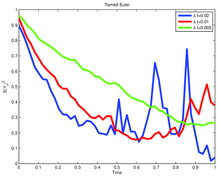
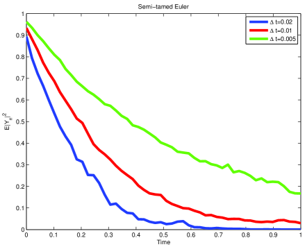
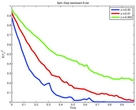
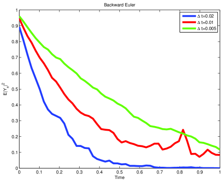
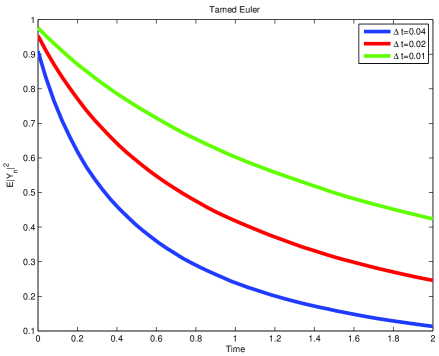
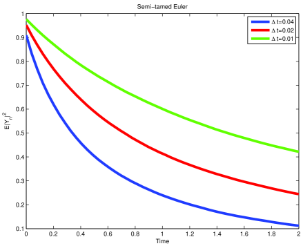
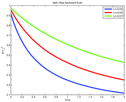
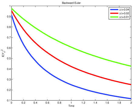
respectively in Section 2 and Section 3. Section 4 presents numerical simulations to sustain the theoretical results. We also
compare the stability behaviors of tamed and semi-tamed schemes with those of backward Euler and split-step backward Euler, this comparison shows
the good behavior of the semi-tamed scheme and therefore confirms the previous study in [7] for SDEs without jump.
2 Linear mean-square stability
Throughout this work, denotes a complete probability space with a filtration .
For all , we denote by , and , for all .
The goal of this section is to find the time
step-size limit for which the tamed Euler scheme and the semi-tamed Euler scheme are stable
in the linear mean-square sense.
For the scalar linear test problem, the concept of A-stability of a numerical method may be interpreted as ”problem
stable method stable for all ”.
We consider the following linear test equation with real and scalar coefficients.
|
|
|
(5) |
where satisfied .
It is proved in [5] that the exact solution of (5) is mean-square stable if and only if
|
|
|
(6) |
Using the discrete form of (5) , the numerical schemes (4) and (3) will be therefore mean-square stable if and
|
|
|
(7) |
The following result provides the time step-size limit for which the semi-tamed scheme (STS) (4) is is mean-square stable.
Theorem 2.1
Assume that , then and the semi-tamed scheme (4) is mean-square stable if and only if
|
|
|
Proof. Applying the semi-tamed Euler scheme to (5) leads to
|
|
|
(8) |
Squaring both sides of (8) leads to
|
|
|
|
|
(9) |
|
|
|
|
|
Taking expectation in both sides of (9) and using the relations , and
with the fact that and are independents leads to
|
|
|
So, the semi-tamed scheme is stable if and only if
|
|
|
That is
.
The following result provide the time step-size limit for which the non compensated tamed scheme (NCTS) (3) is stable.
Theorem 2.2
Assume that , the tamed Euler scheme (3) is mean-square stable if one of the following conditions is satisfied
, and .
and .
Proof. Applying the tamed Euler scheme (3) to equation (5) leads to
|
|
|
(10) |
By squaring both sides of (10) leads to
|
|
|
|
|
|
|
|
|
|
Using the inequality , the previous equality becomes
|
|
|
|
|
|
|
|
|
|
Taking expectation in both sides of the previous equality and using independence and the fact that , , , leads to :
|
|
|
|
|
(11) |
|
|
|
|
|
If , it follows from (11) that
|
|
|
Therefore, the numerical solution is stable if
|
|
|
That is .
If , using the fact that , inequality (11) becomes
|
|
|
(12) |
Therefore, it follows from (12) that the numerical solution is stable if
. That is .
3 Nonlinear mean-square stability
In this section, we focus on the exponential mean-square stability of
the approximation (4).
We follow closely [7, 5] and assume that and .
It is proved in [5] that under the following conditions,
|
|
|
|
|
(37) |
|
|
|
|
|
(38) |
|
|
|
|
|
(39) |
for all , where , and are constants, the exact solution of SDE (1) is nonlinear mean-square stable
if .
Indeed under the above assumptions, we have [5, Theorem 4]
|
|
|
So, if we have and the exact solution is exponentially mean-square stable.
In the sequel of this section, we will use some weak assumptions, which of courses imply that the conditions (37)-(39) hold.
In order to study the nonlinear stability of the semi-tamed scheme (STS), we make also the following assumptions
Assumption 3.1
There exist some positive constants , ,, , , and such that
|
|
|
|
|
|
|
|
|
We denote by and we will always assume that to ensure the stability of the exact solution.
The nonlinear stability of STS scheme is given in the following theorem.
Theorem 3.1
Under Assumptions 3.1 and the further hypothesis ,
for any stepsize ,
there exists a constant such that
|
|
|
and the numerical solution (4) is exponentiallly mean-square stable.
Proof. The numerical solution (4) is given by
|
|
|
where .
Taking the inner product in both sides of the previous equation leads to
|
|
|
|
|
(40) |
|
|
|
|
|
|
|
|
|
|
|
|
|
|
|
|
|
|
|
|
|
|
|
|
|
Using Assumptions 3.1, it follows that
|
|
|
(41) |
|
|
|
|
|
(42) |
|
|
|
|
|
Set .
On we have
|
|
|
(43) |
Therefore using (41), (42) and (43) in (40) yields
|
|
|
|
|
(44) |
|
|
|
|
|
|
|
|
|
|
|
|
|
|
|
|
|
|
|
|
For , which is equivalent to , (44) becomes
|
|
|
|
|
(45) |
|
|
|
|
|
|
|
|
|
|
|
|
|
|
|
|
|
|
|
|
On we have
|
|
|
(46) |
Therefore, using (41), (42) and (46) in (40) yields
|
|
|
|
|
(47) |
|
|
|
|
|
|
|
|
|
|
|
|
|
|
|
|
|
|
|
|
For , which is equivalent to ,
(47) becomes
|
|
|
|
|
(48) |
|
|
|
|
|
|
|
|
|
|
|
|
|
|
|
|
|
|
|
|
Finally, from the discussion above on and , it follows that on , if then we have
|
|
|
|
|
(49) |
|
|
|
|
|
|
|
|
|
|
|
|
|
|
|
|
|
|
|
|
Taking the expectation in both sides of (49) and using the martingale properties of and leads to
|
|
|
|
|
(50) |
|
|
|
|
|
From Assumptions 3.1, we have
|
|
|
So inequality (50) gives
|
|
|
|
|
|
|
|
|
|
|
|
|
|
|
Iterating the previous inequality leads to
|
|
|
for .
The stability occurs if and only if , so we should also have
|
|
|
That is
|
|
|
(51) |
and there exists a constant such that
|
|
|
By the Taylor expansion, as
|
|
|
|
|
|
|
|
|
|
we obviously have .
In order to analyse the nonlinear mean-square stability of the tamed Euler scheme (NCTS), we use the following assumption.
Assumption 3.2
There exist some positive constant , , , , , , and such that :
|
|
|
|
|
|
|
|
|
|
|
|
|
|
|
(52) |
Using Assumption 3.2, we can easily check that the exact solution of (1) is exponentiallly mean-square stable if
.
Theorem 3.2
Under Assumption 3.2, if
, , and , for any stepsize
|
|
|
there exists a constant such that
|
|
|
and the numerical solution (3) is exponentiallly mean-square stable.
Proof. From equation (3), we have
|
|
|
|
|
(53) |
|
|
|
|
|
|
|
|
|
|
Using Assumption 3.2, it follows that
|
|
|
|
|
|
|
|
|
|
|
|
|
|
|
|
|
|
|
|
|
|
|
|
|
|
|
|
|
|
|
|
|
|
|
So from Assumption 3.2, we have
|
|
|
(59) |
Let us define .
On , using Assumption 3.2 we have :
|
|
|
|
|
(60) |
|
|
|
|
|
Therefore using (59) and (60) in (53) yields
|
|
|
|
|
(61) |
|
|
|
|
|
|
|
|
|
|
Since , (61) becomes
|
|
|
|
|
(62) |
|
|
|
|
|
|
|
|
|
|
On , using Assumption 3.2 and the inequality we have
|
|
|
|
|
(63) |
|
|
|
|
|
Therefore, using (59) and (63), (53) becomes
|
|
|
|
|
(64) |
|
|
|
|
|
|
|
|
|
|
For , which is equivalent to ,
(64) becomes
|
|
|
|
|
(65) |
|
|
|
|
|
|
|
|
|
|
From the above discussion on and , it follows that on , if and then we have
|
|
|
|
|
(66) |
|
|
|
|
|
|
|
|
|
|
Taking the expectation in both sides of (66),
using the relation , , and
leads to
|
|
|
|
|
|
|
|
|
|
|
|
|
|
|
Iterating the last inequality leads to
|
|
|
To have the stability of the NCTS scheme, we should also have
|
|
|
That is
|
|
|
and there exists a constant such that
|
|
|
As in the proof of Theorem 3.1, we obviously have .