Amplified and directional spontaneous emission from arbitrary composite bodies:
a self-consistent treatment of Purcell effect below threshold

Abstract

We study amplified spontaneous emission (ASE) from wavelength-scale composite bodies—complicated arrangements of active and passive media—demonstrating highly directional and tunable radiation patterns, depending strongly on pump conditions, materials, and object shapes. For instance, we show that under large enough gain, $\mathcal{PT}$ symmetric dielectric spheres radiate mostly along either active or passive regions, depending on the gain distribution. Our predictions are based on a recently proposed fluctuating volume–current (FVC) formulation of electromagnetic radiation that can handle inhomogeneities in the dielectric and fluctuation statistics of active media, e.g. arising from the presence of non-uniform pump or material properties, which we exploit to demonstrate an approach to modelling ASE in regimes where Purcell effect (PE) has a significant impact on the gain, leading to spatial dispersion and/or changes in power requirements. The nonlinear feedback of PE on the active medium, captured by the Maxwell–Bloch equations but often ignored in linear formulations of ASE, is introduced into our linear framework by a self-consistent renormalization of the (dressed) gain parameters, requiring the solution of a large system of nonlinear equations involving many linear scattering calculations.

Noise in structures comprising passive and active materials can lead to important radiative effects Premaratne and Agrawal (2011), e.g. spontaneous emission (SE) Allen (1973), superluminescence Dicke (1954), and fluorescence Lahoz et al. (2013). Although large-etalon gain amplifiers and related devices have been studied for decades Allen and Peters (1973); Giles and Desurvire (1991); Gutiérrez-Castrejón and Duelk (2006); Wang and Clarkson (2007), there is increased interest in the design of wavelength-scale composites for tunable sources of scattering and incoherent emission Yoo et al. (2011); Ge and Stone (2014), or which serve as perfect absorbers Chong et al. (2010) at mid-infrared and visible wavelengths.

In this paper, we extend a recently developed fluctuating–volume current (FVC) formulation of electromagnetic (EM) fluctuations Polimeridis et al. (2014); Polimeridis et al. (2015a, b); Jin et al. (2015) to the problem of modeling spontaneous emission and scattering from composite, wavelength-scale structures, e.g. metal–dielectric spasers Bergman and Stockman (2003); Stockman (2011, 2013), subject to inhomogeneities in both material and noise properties. We begin by studying amplified spontaneous emission (ASE) from piecewise-constant composite bodies, showing that their emissivity can exhibit a high degree of directionality, depending sensitively on the gain profile and shape of the objects. For instance, we find that under large enough gain, the directivity of parity-time ($\mathcal{PT}$) symmetric spheres can be designed to lie primarily along active or passive regions, depending on the presence or absence of centrosymmetry, respectively. Such composite micron-scale emitters act as tunable sources of incoherent radiation, forming a special class of infrared/visible antennas exhibiting polarization- and direction-sensitive absorption and emission properties. An important ingredient for the design of directional emission is the ability to tune the gain profile of the objects, which can be far from homogeneous in realistic settings. Here, we consider two important sources of inhomogeneities affecting population inversion of atomically doped media: inhomogeneous pump profiles and modifications stemming from changes to the emitters’ local radiative environment. Below threshold, the latter stems primarily from changes to atomic decay rates, which can be either enhanced or suppressed through the Purcell effect (PE) Iwase et al. (2010). Because PE is sensitive to the gain and geometry of the objects, such a dependence manifests as a nonlinear and nonlocal interaction (or feedback) between the atomic medium and the optical environment Gu et al. (2013), which we model within the stationary–phase approximation Cerjan et al. (2015a) via a self-consistent renormalization of the (dressed) atomic parameters. We show that this leads to a system of nonlinear equations, involving as many degrees of freedom as there are volumetric unknowns, which in principle require many scattering problems (radiation from dipoles) to be solved simultaneously, but which thanks to the low-rank nature of volume–integral equation (VIE) scattering operators Polimeridis et al. (2015b) can be accurately obtained with far fewer scattering calculations than there are unknowns. Our predictions indicate that under significant PE, composite objects can exhibit a high degree of dielectric gain enhancement/suppression and inhomogeneity, affecting power requirements and emission patterns.

Gain–composite structures are the subject of recent theoretical and experimental work Premaratne and Agrawal (2011), and have been studied in a variety of different contexts, including spasers (combinations of metallic and gain media) with low-threshold characteristics Bergman and Stockman (2003); Stockman (2011, 2013); Parfenyev and Vergeles (2012); Arnold et al. (2013), random structures with special absorption properties Zaitsev and Deych (2010); Andreasen and Cao (2010); Bachelard et al. (2012); Liew et al. (2014); Ge et al. (2014), and nano-scale particles with highly tunable emission and scattering properties Fan et al. (2010); Prosentsov (2013). $\mathcal{PT}$–symmetric structures have received special attention recently as they shed insights into important non-Hermitian physics, such as design criteria for realizing exceptional points Heiss (2012), symmetry–breaking Heiss (2012), uni-directional scattering Lin et al. (2011); Ge et al. (2012); Alaeian and Dionne (2014), and lasing thresholds Kulishov and Kress (2013). Until recently, most studies of radiation/scattering from $\mathcal{PT}$ structures remained confined to 1d and 2d geometries Chong et al. (2011); Longhi and Feng (2014); Ge et al. (2012); Alaeian and Dionne (2014); Miri et al. (2014); Graefe and Jones (2011); Turduev et al. (2014); Yoo et al. (2011). In such low-dimensional systems, it is common to employ scattering matrix formulations Longhi and Feng (2014); Ge et al. (2012); Chong et al. (2011) to solve for the complex eigenmodes and scattering properties of bodies, leading to many analytical insights. For instance, while the introduction of gain violates energy conservation, a generalized optical theorem can be obtained in 1d, establishing conditions for unidirectional transmission of light Lin et al. (2011); Ge et al. (2012); Alaeian and Dionne (2014). Other studies focus on 2d high–symmetry objects such as cylindrical or spherical bodies Miri et al. (2014); Graefe and Jones (2011) or particle lattices Turduev et al. (2014), demonstrating strong asymmetric and gain-dependent scattering cross-sections, while 3d structures such as ring resonators have been studied within the framework of coupled-mode theory Feng et al. (2014); Peng et al. (2014). With few exceptions Yoo et al. (2011), however, most studies of gain–composite bodies have focused on their scattering rather than emission properties.

Furthermore, while these systems are typically studied under the assumption of piecewise-constant Yoo et al. (2011); Chong et al. (2011); Ge et al. (2012) or linearly varying Ge and Stone (2014) gain profiles, in realistic situations, inhomogeneities in the pump or material parameters (e.g. arising from PE Gu et al. (2013), hole burning Haken (1985); Siegman (1986), and gain saturation Siegman (1986)) result in spatially varying dielectric profiles which alter SE. For example, the highly-localized nature of plasmonic resonances in spasers result in strongly inhomogeneous pumping rates Stockman (2011) and orders-of-magnitude enhancements in atomic radiative decay rates Zhou et al. (2013). In random lasers Zaitsev and Deych (2010), partial pumping plays an important role in determining the lasing threshold Andreasen and Cao (2011); Bachelard et al. (2012) and directionality Liew et al. (2014); Ge et al. (2014). Rigorous descriptions of lasing effects in these systems commonly resort to solution of the full Maxwell–Bloch (MB) equations, in which the electric field $\mathbf{E}$ and induced (atomic) polarization field $\mathbf{P}$ couple to affect the atomic population decay rates Cerjan et al. (2012). However, the MB equations are a set of coupled, time-dependent, nonlinear partial differential equations Esterhazy et al. (2014) which, not surprisingly, prove challenging to solve except in simple situations involving high–symmetry Zhou et al. (2013); Hess et al. (2012) or low-dimensional structures Premaratne and Agrawal (2011). Recently, brute-force FDTD methods have been employed to study the transition from ASE to lasing in 1d random media Andreasen and Cao (2010); Buschlinger et al. (2015), 2d metamaterials Pusch et al. (2012); Hess et al. (2012), photonic crystals Bermel et al. (2006), and more recently, nano-spasers Zhou et al. (2013).

A more recent, general-purpose method that is applicable to arbitrary structures is the steady-state ab-initio laser theory (SALT), an eigenmode formulation that exploits the stationary-inversion approximation to remove the time dependence and internal atomic dynamics of the MB equations Cerjan et al. (2015b, a); Cerjan and Stone (2015), yet captures important nonlinear effects such as hole burning and gain saturation Cerjan et al. (2015a) through effective two-level polarization and population equations de Valcárcel et al. (2006). The resulting nonlinear eigenvalue equation can be solved via a combination of Newton-Raphson Esterhazy et al. (2014); Burkhardt et al. (2015), sparse-matrix solver Hénon et al. (2002), and nonlinear eigenproblem Guillaume (1999) techniques, in combination with either spectral “CF” basis expansions (especially suited for structures with special symmetries) Türeci et al. (2006) or brute-force methods Andreasen and Cao (2009) that can handle a wider range of shapes and conditions. Although this formulation can describe many situations of interest, it nevertheless poses computational challenges in 3d or when applied to structures supporting a large number of modes Esterhazy et al. (2014). Furthermore, the impact of noise below or near threshold has yet to be addressed, although recent progress is being made along these directions Esterhazy et al. (2014); Burkhardt et al. (2015).

Below and near the lasing threshold, however, stimulated emission is often negligible, enabling linearized descriptions of the gain medium Siegman (1986); Campione et al. (2011); Cerjan et al. (2012); Chua et al. (2011). Such approximations, however, ignore nonlinearities stemming from the induced radiation rate $\sim\mathbf{E}\cdot\mathbf{P}$ present in the MB equations, which captures feedback on the atomic medium due to amplification or suppression of noise from changes in the local density of states (also known as Purcell effect) Zhou et al. (2013); Yasumoto (2005); Lau et al. (2008). Here, we show that PE can be introduced into the linearized framework via a self-consistent renormalization or dressing of the gain parameters, an approach that was recently suggested Gu et al. (2013) but which has yet to be demonstrated. In particular, working within the scope of the linearized MB equations and stationary-inversion approximation, we capture the nonlinear feedback of ASE on gain, i.e. the steady-state enhancement/suppresion of gain and atomic decay rates due to PE, via a series of nonlinear equations involving many coupled, linear, classical scattering calculations—local density of states or far-field emission due to electric dipole currents. Since the gain profile can become highly spatially inhomogeneous, it is advantageous to tackle this problem using brute-force methods, e.g. finite differences Taflove et al. (1995), finite elements Chew et al. (2001), or via the scattering VIE framework described below. Our FVC method is particularly advantageous in that it is general and especially suited for handling scattering problems with large numbers of degrees of freedom (defined only within the volumes of the objects), in contrast to eigenmode expansions Türeci et al. (2006) which become inefficient in situations involving many resonances Esterhazy et al. (2014); Türeci et al. (2006) or near-field effects Liu et al. (2015); Khandekar et al. (2015).

I Theory

Active medium.— To begin with, we review the linearized description of a gain medium consisting of optically pumped 4-level atoms: a dense collection of active emitters (e.g. dye molecules Siegman (1986) or quantum dots Strauf and Jahnke (2011); Gregersen et al. (2012)) embedded in a passive (background) dielectric medium $\epsilon_{r}$. (Note that our choice of 4-level system here is merely illustrative since the same approach described below also applies to other active media.) The effective permittivity of such a medium is well described by a simple 2-level Lorentzian gain profile Siegman (1986); Campione et al. (2011); Chua et al. (2011),

$$\epsilon(\omega,\mathbf{x})=\epsilon_{r}(\omega)+\underbrace{\frac{4\pi g(\mathbf{x})^{2}}{\hbar\gamma_{\perp}}\frac{\gamma_{\perp}D_{0}(\mathbf{x})}{\omega-\omega_{21}+i\gamma_{\perp}}}_{\epsilon_{g}(\mathbf{x},\omega)},$$ (1)

where $\epsilon_{g}$ depends explicitly on the frequency $\omega_{12}$, polarization decay rate $\gamma_{\perp}$ (or gain bandwidth), coupling strength $g^{2}=\frac{3\hbar c^{3}}{2\sqrt{\epsilon_{r}}\omega_{21}^{3}}\gamma_{21}^{r}$ Chua et al. (2011); Campione et al. (2011), and inversion factor $D_{0}=n_{2}-n_{1}$ associated with the $2\to 1$ transition. Under the adiabatic or stationary-inversion approximation Cerjan et al. (2015a) and assuming that the system is pumped at $\omega_{30}$, the steady-state population inversion is given by:

$$D_{0} =\frac{\left(1-\frac{\gamma_{21}}{\gamma_{10}}\right)\mathcal{P}/\gamma_{21}}{1+\left(A\frac{\gamma_{21}}{\gamma_{32}}+\frac{\gamma_{21}}{\gamma_{10}}+1\right)\mathcal{P}/\gamma_{21}}n.$$ (2)

(Note that in a dense medium, $\gamma_{\perp}\gg\gamma_{21}$ is dominated by collisional and dephasing effects Siegman (1986).) Here, $A=1(2)$ for incoherent (coherent) pump source; $c$ denotes the speed of light, $n_{i}$ the population (per unit volume) of level $i$, $n=\sum_{i}n_{i}$ the overall atomic population, $\gamma_{ij}=\gamma_{ij}^{r}+\gamma_{ij}^{nr}$ the decay rate from level $i\to j$, consisting of radiative and non-radiative terms, respectively, and $\mathcal{P}(\mathbf{x})=\frac{\sigma c}{\sqrt{\epsilon_{r}(\omega_{30})}\hbar\omega_{30}}|E(\mathbf{x},\omega_{30})|^{2}$ is the position-dependent pump rate from $0\to 3$, which is often the main source of spatial dispersion.

The SE properties of such a medium are described by the fluctuation–dissipation theorem (FDT) Matloob et al. (1997); Jeffers et al. (1993); Graham and Haken (1968). In particular, from local thermodynamic considerations, one can show that associated with the presence of absorption or amplification are fluctuating polarization currents $\sigma$ whose correlation functions, $\langle\sigma_{i}(\mathbf{x},\omega)\sigma_{j}^{\ast}(\mathbf{y},\omega)\rangle=\frac{4}{\pi}\operatorname{Im}\epsilon_{g}(\mathbf{x},\omega)n_{2}/(n_{1}-n_{2})\delta(\mathbf{x}-\mathbf{y})\delta_{ij}$, depend on the corresponding macroscopic gain profile $\operatorname{Im}\epsilon_{g}$ and population inversions $n_{2}/(n_{1}-n_{2})$. The latter is often described in terms of an effective (local) temperature $T$ defined with respect to the Planck spectrum Matloob et al. (1997), $(e^{\hbar\omega/k_{\mathrm{B}}T}-1)^{-1}$, whose value turns negative Patra and Beenakker (1999) for systems with population inversion $n_{2}>n_{1}$, where $T\to 0^{-}$ in the limit of complete inversion Jeffers et al. (1993). The presence of inhomogeneities in the dielectric function and fluctuation statistics can be a hurdle for calculations of SE that rely on scattering-matrix formulations Bimonte (2009); Messina and Antezza (2011), but here we exploit a recently developed FVC formulation based on the VIE method which captures all of the relevant physics.

FVC formulation.— In order to obtain the individual and/or cummulative radiation from all dipoles within a given object, we exploit the FVC formulation introduced in Polimeridis et al. (2015b) and summarized here. The starting point of FVC is the VIE formulation of EM scattering Chew et al. (2001), describing scattering of an incident, 6-component electric ($\mathbf{E}$) and magnetic ($\mathbf{M}$) field $\phi_{\rm inc}=(\mathbf{E};\mathbf{H})$ from a body described by a spatially varying $6\times 6$ susceptibility tensor $\chi(\mathbf{x})$. Given a 6-component electric ($\mathbf{J}$) and magnetic ($\mathbf{M}$) dipole source $\sigma=(\mathbf{J};\mathbf{M})$, the incident field is obtained via a convolution ($\star$) with the $6\times 6$ homogeneous Green’s function (GF) of the ambient medium $\Gamma(\mathbf{x},\mathbf{y})$, such that $\phi_{\mathrm{inc}}=\Gamma\star\sigma=\int d^{3}\mathbf{y}\Gamma(\mathbf{x},\mathbf{y})\sigma(\mathbf{y})$. Exploiting the volume equivalence principle Chew et al. (2001), the unknown scattered fields $\phi_{\rm sca}=\Gamma\star\xi$, can also be expressed via convolutions with $\Gamma$, except that here $\xi=-i\omega\chi\phi$ are the (unknown) bound currents in the body, related to the total field inside the body $\phi=\phi_{\mathrm{inc}}+\phi_{\mathrm{sca}}$ through $\chi$. Writing Maxwell’s equations in terms of the bound currents, we arrive at the so-called JM–VIE equation Polimeridis et al. (2014):

$$\underbrace{\left[\Gamma\star+(i\omega\chi)^{-1}\right]}_{Z}\xi=-(\Gamma\star\sigma),$$ (3)

whose solution can be obtained by a Galerkin discretization of the currents $\sigma(\mathbf{x})=\sum_{n}s_{n}b_{n}(\mathbf{x})$ and $\xi(\mathbf{x})=\sum_{n}x_{n}b_{n}(\mathbf{x})$ in a convenient, orthonormal basis $\{b_{n}\}$ of $N$ 6-component vectors, with vector coefficients $s$ and $x$, respectively. The resulting matrix expression has the form $x+s=Ws$, where the VIE matrix $({W}^{-1})_{m,n}=\langle b_{m},b_{n}+i\omega\chi(\Gamma\star b_{n})\rangle$ and $\langle,\rangle$ denotes the standard conjugated inner product. Direct application of Poynting’s theorem yields the following expression for the far-field radiation flux from $\sigma$ (here, a single dipole source embedded within the volume) Jackson (1998):

$$\Phi_{\sigma}=-\frac{1}{2}\text{Tr }\left[DW^{*}\operatorname{sym}GW\right]$$ (4)

where $D=s^{*}s$ and $G$ are $N\times N$ matrices, with ${G}_{mn}=\langle b_{m},\Gamma\star b_{n}\leavevmode\nobreak\ \rangle$.

If $\{b_{n}\}$ is chosen to be a localized basis of unit-amplitude, i.e. $\langle b_{m},b_{n}\rangle=\delta_{nm}$, volume elements, then the flux contribution from a given dipole source in the volume (including different polarizations) $b_{n}$ is precisely the diagonal element $-\frac{1}{2}(W^{*}\operatorname{sym}GW)_{n,n}$. In contrast, the overall ASE is given by an ensemble-average over all such fluctuating dipole sources $\Phi=\langle\Phi_{\sigma}\rangle$, in which case the elements of the matrix ${D}$, which encodes information about the current amplitudes, are given by the current–current correlations $\langle{D}\rangle_{mn}=\int\int d^{3}\mathbf{x}d^{3}\mathbf{y}\,b_{m}^{\ast}(\mathbf{x})\langle\sigma(\mathbf{x})\sigma^{\ast}(\mathbf{y})\rangle b_{n}(\mathbf{y})$, determined by the FDT above. Direct computation of (4) is expensive due to the large dimensionality $N$ of the problem, but it turns out that the Hermitian, negative-semidefinite, and low-rank nature of $\operatorname{sym}G$ (since it is associated with the smooth, imaginary part of the Green’s functions) enables re-expressing the trace as the Frobenius norm of a low-rank matrix. Specifically, decomposing $\operatorname{sym}G=-U_{r}S_{r}U_{r}^{*}$ via a fast approximate SVD Hochman et al. (2014), where $r\ll N$ Chai and Jiao (2013), and further decomposing $S_{r}=L_{S}L_{S}^{*}$, we find that the product $W^{*}\operatorname{sym}GW$ can be written in the form $QQ^{*}$, with $Q=W^{*}U_{r}L_{S}$, reducing the calculation of the diagonal elements to a small series $r\ll N$ of scattering calculations (matrix-inverse operations) Polimeridis et al. (2014). Similarly, as shown in Polimeridis et al. (2015b), the same follows for the overall ASE which is just a weighted sum of the diagonal elements. For example, while the calculations below require $N\geq 40^{3}$ basis functions to obtain accurate spatial resolution, we find that generally $r\lesssim 20$.

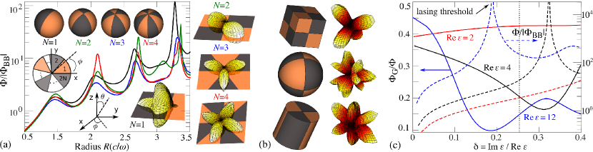
Figure 1: (a) SE flux $\Phi$ from $\mathcal{PT}$–symmetric spheres consisting of $N=\{1,2,3,4\}$ (black, green, blue, and red lines) regions of equal gain (red) and loss (blue), with permittivities $\epsilon=4\pm i$ and gain temperature $T\to 0^{-}$ K (corresponding to complete population inversion), as a function of sphere radius $R$ (for a fixed vacuum wavelength $2\pi c/\omega$). $\Phi(\omega)$ is normalized by the flux $|\Phi_{\mathrm{BB}}(\omega)|=R^{2}(\omega/c)^{2}\hbar\omega$ from a “blackbody” of the same surface area and temperature. Insets show angular radiation intensities $\Phi(\theta,\phi)$ for different $N$ at selective radii $R=\{2.6,3,2.7,2.1\}(c/\omega)$ (corresponding to increasing $N$), with orange/gray colormaps denoting regions of gain/loss. (b) Selected $\Phi(\theta,\phi)$ of various $\mathcal{PT}$–symmetric shapes, including “beach balls”, “magic” cubes, and cylinders, showing complex directivity patterns that depend strongly on the centro-symmetry of the objects. Here the color white (black) refers to the maximum (minimum) flux value. (c) Peak SE flux $\Phi$ (right axis, dashed lines) and directivity $\Phi_{G}/\Phi$ (left axis, solid lines), or the ratio of the flux emitted along gain direction $\Phi_{G}$ (see text) to the total flux $\Phi$, near the third resonance of the $N=1$ sphere, as a function of the gain/loss tangent $\delta=|\operatorname{Im}\epsilon|/\operatorname{Re}\epsilon$ and for multiple values of $\operatorname{Re}\epsilon=\{2,4,12\}$ (red, black, and blue lines), where the vertical dashed black line denotes $\delta$ for (a). The plots show increased directivity attained as the system approaches the lasing threshold (marked in the case of $\operatorname{Re}\epsilon=12$, where $\Phi$ diverges ).

Purcell effect.— Although often assumed to be uniform, the atomic radiative decay rates $\gamma_{ij}^{r}$ entering (1) are in fact position dependent due to PE Yasumoto (2005); Zhou et al. (2013), leading to changes in the dipole coupling $g$ and population inversion factor $D_{0}$, either enhancing or suppressing (quenching) gain Yasumoto (2005). In what follows, we only consider modifications to the radiative decay rate at the lasing transition $\gamma_{21}^{r}$; unlike the pump which is incident at a non-resonant frequency, changes in $\gamma_{21}^{r}$ can have a significant impact on SE and must therefore be treated self-consistently.

The impact of PE on the radiative decay rate $\gamma^{r}_{21}$ of an atom at some position $b_{n}$ is captured by the coupling of the atomic polarization and electric fields $\sim\mathbf{P}\cdot\mathbf{E}$, or the induced radiation term in the MB equations, in the presence of the noise and surrounding dielectric environment Waks and Sridharan (2010). While technically this requires abandoning the linear model above, the weak nature of noise (ignoring stimulated emission) implies that the latter can also be obtained (perturbatively) from a linear, classical calculation: the radiative flux $\Phi_{b_{n}}$ from a classical dipole at $b_{n}$. Specifically, the renormalized or dressed decay rate of an atom at position $\mathbf{x}$ can be expressed as Yasumoto (2005):

$$\gamma^{r}_{21}(\mathbf{x})=\mathcal{F}(\mathbf{x})\gamma^{r,0}_{21},$$ (5)

where $\mathcal{F}(\mathbf{x})$ denotes the Purcell factor of a dipole at $\mathbf{x}$, and the supper-script “0” denotes the decay rate of the atomic population in the lossy (background) medium. It follows that the decay rate associated with a given $b_{n}$ and entering (1) is given by $\gamma_{21}(b_{n})=\gamma_{21}^{nr}+\mathcal{F}_{b_{n}}\gamma_{21}^{r,0}$, where the Purcell factor,

$$\mathcal{F}_{b_{n}}=\Phi_{b_{n}}/\Phi^{0}.$$ (6)

(Note that all $\Phi_{b_{n}}\sim(W^{*}\operatorname{sym}GW)_{n,n}$ can be computed very fast, as explained above.) Here, we assume that the bulk (background) medium $\epsilon_{r}$ only has a significant impact on $\gamma^{nr,0}_{21}$ (obtained either experimentally or theoretically by accounting for atomic interactions within the bulk) Siegman (1986) but not on the radiative decay rate $\gamma^{r,0}_{21}$, in which case $\Phi^{0}=\omega^{4}/12\pi\epsilon_{0}c^{3}$ is the emission rate of the atom in vacuum (assuming a unit-amplitude dipole). Note that in a lossy medium, e.g. in metals, the bare $\gamma^{0}_{21}$ will be dominated by non-radiative processes Wu et al. (2009); Fang et al. (2012), leading to small quantum yields (QY) $\gamma^{r,0}_{21}/\gamma^{0}_{21}\ll 1$. Note also that technically, the calculation of the Purcell factor requires integration over the gain bandwidth, $\mathcal{F}_{b_{n}}=\int d\omega\frac{\gamma_{\perp}/\pi}{\gamma_{\perp}^{2}+(\omega-\omega_{21})^{2}}\frac{\Phi_{b_{n}}(\omega)}{\Phi^{0}(\omega)}$, but here we make the often-employed and simplifying assumption that $\gamma_{\perp}\gg\gamma_{21}$ and $\gamma_{\perp}\lesssim$ spectral radiative features Lu et al. (2014); Kristensen et al. (2013), so as to only consider radiation at $\omega_{21}$.

The gain profile of a body subject to an incident pump rate $\mathcal{P}$ can be obtained by enforcing that (1) and (5) be satisfied simultaneously. Such systems of nonlinear equations are most often solved iteratively using one or a combination of algorithms, ranging from simple fixed-point iteration Süli and Mayers (2003) to more sophisticated approaches like Newton–Raphson and nonlinear Arnoldi methods Esterhazy et al. (2014); Voss (2004). Essentially, starting with the bare parameters, dressed decay rates are computed via (5) from the radiation equation (4) after which, having updated the gain–medium equation (1), the entire process is repeated until one arrives at a fixed-point of the system. In principle, this requires hundreds of thousands $N$ of scattering calculations (flux from each dipole source in the active region) to be solved per iteration, which becomes prohibitive in large systems, but the key here is that the entire spatially varying flux $\{\Phi_{b_{n}}\}$ throughout the body can be computed extremely fast, requiring far fewer ($\ll N$) scattering calculations (as described above). Note that these large systems of nonlinear equations have many fixed points and hence convergence to the correct solution is never guaranteed, depending largely on the inital guess and algorithm employed Walker and Iteration (2011). However, a convenient and effective approach is to begin by first solving the system in the fast-converging (passive) regime $\mathcal{P}n/\gamma_{12}\ll 1$, and then employing this solution as an initial guess at larger pumps.

II Results

We begin this section by showing that wavelength-scale composite bodies can exhibit highly complex, tunable, and directional radiation patterns. Although it is not surprising that objects undergoing ASE (once known as “mirrorless lasers”) exhibit highly directed radiation patterns Ramachandran (2002), few studies have gone beyond large-etalon Fabry-Perot cavities Zhu et al. (2013) or fiber waveguides Harrington (2004), often modelled via ray-optical or scalar-wave equations Premaratne and Agrawal (2011), which miss important effects present in wavelength-scale systems Esterhazy et al. (2014). Further below, we show that dielectric inhomogeneities arising from the pump and/or radiation process can also introduce important changes to the ASE patterns. In particular, we apply the renormalization approach described above to consider the nonlinear impact of Purcell effect on the gain medium, and show that while in many cases a homogeneous approximation leads to accurate results, there are situations where these can fail dramatically. Our calculations are only meant to serve as proof of principle and revolve around highly doped (Er³⁺ and Rhodamine) but simple dielectric objects, allowing faster computations but requiring very large values of $\operatorname{Im}\epsilon_{g}$ to achieve significant gain. Similar results follow, however, in systems subject to smaller $\epsilon_{g}$ or smaller doping densities, at the expense larger pump powers or by exploiting resonances with greater confinement or smaller radiative loss rates (e.g. compact bodies of larger dimensions and/or refractive indices, or more complex structures such as photonic-crystal resonators).

Tunable radiation patterns.— We begin by exploring SE from piecewise-constant $\mathcal{PT}$–symmetric spheres [Fig. 1 insets] consisting of a background dielectric medium, e.g. nano-composite polymers Zhang et al. (2012); Macdonald and Shaver (2015) or semiconductors Eliseev and Van Luc (1995); Feng et al. (2014), doped with active materials to realize different ($N$) regions of equal gain (red) or loss (blue). Figure 1(a) shows the SE flux $\Phi$ from spheres of varying $N=\{1,2,3,4\}$ (black, green, blue, red lines) and gain/loss permittivities $\epsilon=4\pm i$, at a fixed frequency $\omega$ and gain temperature $T\to 0^{-}$ K (corresponding to complete inversion), as a function of radius $R$ (in units of the vacuum wavelength $c/\omega$). $\Phi(\omega)$ is normalized by the flux $|\Phi_{\mathrm{BB}}(\omega)|=R^{2}(\omega/c)^{2}\hbar\omega$ from a “blackbody” of the same surface area and temperature. As expected, $\Phi$ exhibits peaks at selected $R\gtrsim(c/\omega)$ corresponding to enhanced emission at Mie resonances. (Note that peaks in $\Phi$ continue to increase in amplitude with increasing $R$, due to decreased radiative losses, with the bandwidth of the resonances narrowing as the system reaches the lasing transition, at which point our linear approach breaks down.) Associated with increased ASE is increased directivity, illustrated by the radiation patterns $\Phi(\theta,\phi)$ shown on the insets of Fig. 1(a) at selected $R$, whose high directionality contrast sharply with the emission profile of passive particles. (With few exceptions Jin et al. (2015), the latter tend to emit quasi-isotropically, as can be verified by decreasing the gain of the spheres.) We find that the direction of largest ASE changes drastically with respect to $N$, with radiation coming primarily from either active or passive regions depending on whether the spheres exhibit or lack centrosymmetry, respectively (insets). In particular, the ratio $\Phi_{G}/\Phi$ of the flux emitted from the gain surfaces,

$$\Phi_{G}=\sum_{k=0}^{N-1}\int d\theta\sin^{2}(\theta)\int_{2\pi k/N}^{\pi(2k+1)/N}d\phi\,\Phi(\theta,\phi),$$

to the total flux $\Phi$, is generally $\lesssim 0.5$ for odd $N$ (centrosymmetric) and $\gtrsim 0.5$ otherwise. For instance, $N=1$ spheres exhibit $\Phi_{G}/\Phi\approx 0.1$ at $R\approx 3.3(c/\omega)$ whereas $N=2$ spheres exhibit $\Phi_{G}/\Phi\approx 0.75$ at $R\approx 3(c/\omega)$. The sensitive dependence of emission pattern on geometry and gain profile is not unique to spherical structures, as illustrated in Fig. 1(b), which shows $\Phi(\theta,\phi)$ for various shapes, including “magic” cubes, “beach balls”, and cylinders—as before, the presence/absence of centro-symmetry results in high/low gain directivity.

To understand the features and origin of these emission patterns, Fig. 1(c) explores the dependence of the peak $\Phi$ (dashed lines) and $\Phi_{G}/\Phi$ (solid lines) on the gain/loss tangent $\delta=|\operatorname{Im}\epsilon|/\operatorname{Re}\epsilon$ of the $N=1$ sphere, near the third resonance and for multiple values of $\operatorname{Re}\epsilon=\{2,4,12\}$. As shown, there is negligible ASE in the limit $\operatorname{Im}\epsilon\to 0$, yet the localization of fluctuating dipoles to the gain-half of the (increasingly uniform) sphere leads to a small (though observable) amount of directionality, favoring emission toward the loss direction. The tendency of dipoles within a sphere to emit in a preferred direction has been studied in the context of fluorescence Lock (2001) in the ray-optical limit $R\gg c/\omega$, which as shown here is exacerbated in the presence of gain Chen et al. (2012): essentially, dipoles within a sphere tend to emit in the direction opposite the nearest surface, which explains why spheres having/lacking centro-symmetry tend to emit along directions of gain/loss. Moreover, in order to achieve large directivity, there needs to be a significant amount of mode confinement and gain, as illustrated by the negligible ASE and directivity of the $\operatorname{Re}\epsilon=2$ sphere. Finally, we find that for large enough $\operatorname{Re}\epsilon$, the directivity increases with increasing $\operatorname{Im}\epsilon$, peaking at a critical $\delta$, corresponding to the onset of lasing. Such a transition is marked by a diverging $\Phi$ near the threshold along with a corresponding narrowing of the resonance linewidth (not shown). (Note that our predictions close to and above this critical gain are no longer accurate since they neglect important effects stemming from stimulated emission Grynberg et al. (2010). For instance, at and above the critical gain, the resonance linewidth goes to zero and then broadens with increasing $\operatorname{Im}\epsilon$, while it is well known that nonlinear gain saturation results in a finite laser linewidth Cerjan et al. (2015b); Cerjan and Stone (2015)) Nevertheless, our results demonstrate that a significant amount of directivity can be obtained below the onset of lasing, where the linear approximation is still valid.

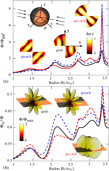
Figure 2: (a) SE flux $\Phi$ and (b) gain directivity $\Phi_{G}/\Phi$, or the ratio of the flux emitted along the gain directions $\Phi_{G}$ (see text) to the total flux $\Phi$, from the $N=2$ sphere (inset) of Fig. 1 at frequency $\omega_{21}$, corresponding to the transition frequency of an active region consisting of Rhodamine 800 dye molecules. The gain medium is excited by planewaves propagating in opposite directions, $\mathbf{x}\cos\phi+\mathbf{y}\sin\phi$ and $-\mathbf{x}\cos\phi-\mathbf{y}\sin\phi$, for three different orientations, $\phi=0$ (black line), $\pi/4$ (blue line), and $-\pi/4$ (red line), leading to significant spatial inhomogeneities. $\Phi$ is normalized by $\Phi_{\mathrm{BB}}$ as in Fig. 1 and plotted as a function of radius $R$, in units of the dye $2\to 1$ transition wavelength $c/\omega_{21}$ (see text). Insets in (a) show $z=0$ cross-sections of the resulting gain profiles $-\mathrm{Im}\epsilon_{g}$ at $R=3.4(c/\omega_{21})$ while those in (b) show angular radiation intensities $\Phi(\theta,\phi)$ normalized by the maximum intensity $\Phi_{max}$ at $R=4(c/\omega_{21})$ for the different pump orientations.

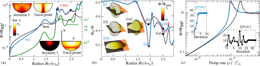
Figure 3: Self-consistent treatment of Purcell effect (PE) based on solution of (1) and (5) using fixed-point iteration. (a) SE flux $\Phi$ normalized by $\Phi_{\mathrm{BB}}$ as in Fig. 1 and (b) gain directivity $\Phi_{G}/\Phi$ from the $N=1$ sphere of Fig. 1, as a function of radius $R$ (in units of $c/\omega_{21}$), with an active medium consisting of Er³⁺ atoms and subject to a uniform pump rate $\mathcal{P}/\gamma^{0}_{21}=10^{-4}$, where $\omega_{21}$ and $\gamma^{0}_{21}$ denote the bulk (bare) $2\to 1$ transition frequency and decay rate of the atoms, respectively. Top/bottom insets in (a) show $z=0$ cross-sections (contour plots) of the gain profiles $-\mathrm{Im}\epsilon_{g}$ obtained during the first and final (fixed-point) iteration of the algorithm at two separate radii $R=\{2,2.5\}(c/\omega_{21})$, with black/white denoting $\min,\max-[\operatorname{Im}\epsilon_{g}]\approx\{1.9,1.3\}$ and $\{1.9,1.5\}$, respectively. Insets in (b) show the angular radiation intensities $\Phi(\theta)$ at selected radii (black dots), normalized by the maximum intensity $\Phi_{max}$. (c) $\Phi$ at a fixed radius $R=2(c/\omega_{21})$ as a function of $\mathcal{P}/\gamma_{21}^{0}$, with insets illustrating the evolution of $\Phi$ as a function of iteration at a fixed $\mathcal{P}/\gamma^{0}_{21}=10^{-4}$ and for two different values of quantum yields (QY) [see text]. All plots compare quantities in the presence (solid blue lines) or absence (dashed black lines) of PE, and under a uniform–medium approximation (UMA) (solid red lines) described in the text; the solid green line in (a) denotes the average Purcell factor $\langle\mathcal{F}\rangle=\frac{1}{V}\int_{V}\mathcal{F}$ at each radius.

Pump inhomogeneity.— Next, we employ the 4-level gain model of (1) to illustrate the impact of gain inhomogeneities on ASE. While both $\mathcal{P}$ and PE are simultaneous sources of spatial dispersion, for the sake of comparison we consider each independently of one another. We begin by studying the impact of pump on the $N=2$ sphere (above) for an active region consisting of a background medium $\epsilon_{r}=4$ that is doped with Rhodamine 800 dye molecules with atomic parameters: $\omega_{21}=2.65\times 10^{15}s^{-1}$ ($\lambda\approx 711$ nm), $\gamma_{\perp}/\omega_{21}=0.04$ , $\gamma_{21}/\omega_{21}=7.5\times 10^{-7}$, $\gamma_{32}/\omega_{21}=\gamma_{10}/\omega_{21}=10^{-3}$, QY of 20%, and concentration $n=40$ mM ($2.4\times 10^{19}$ cm^-3) Campione et al. (2011). Note that since $\omega_{30}\gg\omega_{21}$, it is safe to neglect feedback due to PE and hence $\mathcal{P}$ is determined from a single scattering calculation Polimeridis et al. (2015b). For these parameters Campione et al. (2011), a pump rate $\mathcal{P}/\gamma_{21}\approx 1$ results in $-\operatorname{Im}\epsilon_{g}(\omega_{21})\approx 1$. We consider illumination with $\mathbf{z}$-polarized planewaves incident from two opposite directions along the $x$–$y$ plane, shown schematically in Fig. 2. The insets depict $z=0$ cross-sections of the resulting $\epsilon_{g}$ profile [Fig. 2(a)] at $R=3.4(c/\omega_{21})$ along with emission patterns $\Phi(\theta,\phi)$ [Fig. 2(b)] at $R=4(c/\omega_{21})$, under three incident conditions, corresponding to different directions of incidence, $\hat{\mathbf{x}}\cos\phi+\hat{\mathbf{y}}\sin\phi$ and $-\hat{\mathbf{x}}\cos\phi-\hat{\mathbf{y}}\sin\phi$, with $\phi=\{0,\pm\pi/4\}$; in each case, the incident power is chosen such that $\mathrm{max}\{-\mathrm{Im}[\epsilon_{g}]\}=1$. As shown, the gain profiles vary dramatically with respect to position and incident angle, with $\operatorname{Im}\epsilon_{g}$ changing from $0\to 1$ on the scale of the wavelength. These spatial variations lead to correspondingly large changes in the overall ASE [Fig. 2(a)] and directivity [Fig. 2(b)]. More importantly, we find that these features cannot be explained by naive, uniform–medium approximations (UMA). For instance, replacing $\epsilon_{g}$ with the average gain $\langle\epsilon_{g}\rangle=\frac{1}{V}\int_{V}\epsilon_{g}$ in the case $\phi=-\pi/4$, we find that UMA predicts an emission rate $\Phi/\Phi_{\mathrm{BB}}\approx 30$ that is three times larger than that predicted by exact calculations. Differences in illumination angle also result in different angular radiation patterns $\Phi(\theta,\phi)$. For instance, we find that $\phi=-\pi/4$ leads to much more isotropic radiation than $\phi=\{0,\pi/4\}$, a consequence of the larger $\operatorname{Im}\epsilon_{g}$ near the center of the sphere and the fact that dipoles near the center tend to radiate more isotropically and efficiently than those which are farther laying farther away.

Purcell effect.— We now consider inhomogeneities arising from PE, assuming a uniform pump and doping concentration. In particular, we apply the self-consistent framework described in Sec. I to study ASE from the $N=1$ sphere above, but with an active region consisting of a background medium $\epsilon_{r}=4$ that is doped with Er³⁺ atoms Godard (2007); Cerjan et al. (2012), with parameters: $\omega_{21}=6.28\times 10^{14}s^{-1}$ ($\lambda\approx 2.8\mu$m), $\gamma_{\perp}/\omega_{21}=0.03$, $\gamma_{21}/\omega_{21}=5\times 10^{-5}$, $\gamma_{32}/\omega_{21}=\gamma_{10}/\omega_{21}=1$, bare QY of 50%, and concentration $n=10^{19}$ cm^-3. (Further below we also consider a different geometry, a metal-dielectric spaser consisting of similar gain parameters but passive metallic regions.) Here, a pump rate $\mathcal{P}/\gamma_{21}=10^{-4}$ results in $-\operatorname{Im}\epsilon_{g}(\omega_{21})\approx 1$ in the absence of PE. As discussed above, we employ fixed-point iteration to solve (4) and (5) and hence obtain consistent values of $\epsilon_{g}$ and $\Phi$, starting with the bare ($\mathcal{F}=1$) atomic parameters and iterating until the gain parameters converge to the nearest fixed point. Generally, the convergence rate of the fixed-point algorithm depends sensitively on the chosen parameter regime, requiring larger number of iterations with decreasing $\frac{\partial\epsilon_{g}}{\partial\gamma_{21}^{r}}$ (decreasing local slope) Süli and Mayers (2003). The convergence also depends on the degree of nonlinearity in the system, which in the case of our 4-level system can be significant under small QY ($\gamma^{r}_{21}/\gamma_{21}\ll 1$), large $\mathcal{P}$, or $\gamma_{21}/\gamma_{10}\lesssim 1$ (in which case there is significant gain saturation). Nevertheless, in practice we find that for a wide range of parameters, a judicious combination of fixed-point iteration and Anderson acceleration Walker and Iteration (2011) ensures convergence within dozens of iterations. The bottom/top insets of Fig. 3(c) demonstrate the iterative process at a fixed $R=2(c/\omega_{21})$ and for two different sets of concentrations $n=\{1,5\}\times 10^{19}$ cm^-3 and quantum yields $\approx\{10,50\}\%$.

Figure 3 illustrates the impact of PE on the emission of the sphere, showing variation in (a) SE flux $\Phi(\omega_{21})$ and (b) gain directivity $\Phi_{G}/\Phi$ of the sphere with respect to radius $R$ at a fixed $\mathcal{P}/\gamma^{0}_{21}=10^{-4}$, or with respect to (c) pump rate $\mathcal{P}$ at a fixed $R=2(c/\omega_{21})$, both including (solid blue lines) and excluding (dashed black lines) PE. As before, $\Phi$ is normalized by $\Phi_{\mathrm{BB}}$. Shown as insets in Fig. 3(a) are $z=0$ cross sections of $\operatorname{Im}\epsilon_{g}$ for the first and final (fixed-point) iteration of the algorithm, at two different radii $R=\{2,2.5\}(c/\omega_{21})$ (black dots), demonstrating large gain enhancement and spatial variations. As expected, $\Phi$ is either enhanced or suppressed depending on the average PE (green line) which we have defined as $\langle\mathcal{F}\rangle\neq 1$, where for convenience we have defined:

$$\langle\mathcal{F}\rangle=\frac{1}{V}\int_{V}\mathcal{F}=\frac{1}{N}\sum_{n}\Phi_{b_{n}}/\Phi^{0}=-\frac{1}{2N\Phi^{0}}\text{Tr }W^{*}\operatorname{sym}GW.$$

(As discussed above, $\langle\mathcal{F}\rangle\sim\Phi$ turns out to be the Frobenius norm of a low-rank matrix and is therefore susceptible to fast computations.) As shown, at small $R\lesssim 1.2(c/\omega_{21})$, or in the absence of resonances, $\langle\mathcal{F}\rangle<1$ and hence $\Phi$ is suppressed with respect to the predictions of the bare. Conversely, $\langle\mathcal{F}\rangle>1$ near resonances and hence $\Phi$ is enhances. Note that for our choice of parameters, the gain profile scales linearly with the quantum yield, i.e. $\epsilon_{g}\propto\mathrm{QY}=\gamma_{21}^{r}/\gamma_{21}$, such that in the limit as $\langle\mathcal{F}\rangle\to\infty$ (ignoring quenching occurring as $\gamma_{21}^{r}\to\gamma_{10}$), $-\operatorname{Im}\epsilon_{g}\to 2$. (For smaller $\mathrm{QY}\ll 1$, $\epsilon_{g}$ can be many times larger than the bare permittivity with increasing $\langle\mathcal{F}\rangle$, saturating at much larger values of PE.) In addition to changing the overall SE rate, PE also modifies the sphere’s directivity. This is illustrated in Fig. 3(b), which shows enhancements in $\Phi_{G}/\Phi$ and correspondingly changes in emission patterns (insets) at selective $R=\{2,2.5\}(c/\omega_{21})$.

Figure 3(c) also explores the dependence of $\Phi$ on $\mathcal{P}$ at a fixed $R=2(c/\omega_{21})$, showing that $\Phi$ peaks at a finite value of $\mathcal{P}/\gamma^{0}_{12}\gtrsim 10^{-4}$ and then decreases with increasing $\mathcal{P}$; the same is true for $\langle\mathcal{F}\rangle$ and $\langle\epsilon_{g}\rangle$ (not shown). Such a non-monotonicity stems from the fact that near the critical pump rate, $\operatorname{Im}\epsilon_{g}\approx\operatorname{Re}\epsilon_{g}$, causing the resonance frequency to shift to smaller radii, a trend that is observed both in the presence and absence of PE. Surprisingly, however, we find that while PE causes large inhomogeneities in $\epsilon_{g}$, in both scenarios the peak emission is approximately the same, suggesting the possibility that one could explain the impact of PE by a simple UMA. In what follows, we exploit a UMA that not only greatly simplifies the calculation of PE but also leads to accurate results over a wider range of parameters. In particular, we consider a UMA in which the otherwise inhomogeneous gain profile of the object is replaced with that of a uniform medium $\epsilon_{g}(\mathbf{x})\to\langle\epsilon_{g}\rangle$ (assuming a uniform pump rate) given by (1) but with $\gamma^{r}_{21}\to\langle\gamma^{r}_{21}\rangle=\langle\mathcal{F}\rangle\gamma^{r,0}_{21}$, corresponding to a homogeneous broadening/narrowing of the gain atoms throughout the sphere. Within this approximation, the system of nonlinear equations above is described by a single (as opposed to $N\gg 1$) degree of freedom $\langle\gamma^{r}_{21}\rangle$, enabling faster convergence along with application of algorithms that are especially suited for handling low-dimensional systems of equations Conn et al. (2009). Ignoring other sources of inhomogeneity (e.g. induced by density or pump variations), such an approximation allows calculation of $\Phi$ via scattering formulations best-suited for handling piecewise-constant dielectrics, including SIE Rodriguez et al. (2013) and related scattering matrix Bimonte (2009) methods. The solid red lines in Fig. 3 are obtained by employing the UMA, demonstrating its validity over a wide range of parameters. Surprisingly, we find that this holds even in regimes marked by strong gain saturation (e.g. $\gamma_{10}\lesssim\gamma_{21}$). It follows that in this geometry, the effect of PE on radiation can be attributed primarily to the presence of a larger average gain or pump rate in the sphere, whereas the actual spatial variation in $\epsilon_{g}$ is largely unimportant.

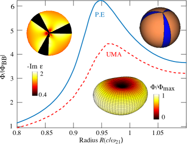
Figure 4: Self-consistent treatment of Purcell effect (PE) obtained from solution of (1) and (5) (solid blue lines) or by the uniform-medium approximation (dashed red line) described in the text. SE flux $\Phi$ from a metal–dielectric composite (top-right inset) as a function of radius $R$ (in units of $c/\omega_{21}$), with orange and blue denoting Er³⁺–doped polymer and Au regions, respectively. Insets show a $z=0$ cross-section of the gain profile $-\mathrm{Im}\epsilon_{g}$ (top) and the angular radiation intensity $\Phi(\theta,\phi)$ (bottom) at $R=0.95(c/\omega_{21})$ normalized by the maximum intensity $\Phi_{max}$.

There are geometries and situations where such a UMA is expected to fail, e.g. structures subject to even large dielectric inhomogeneities (as in Fig. 2). Such conditions arise in large objects (supporting higher-order resonances) or in metal–dielectric composites (supporting highly localized surface waves). Figure 4 shows $\Phi$ for one such structure [bottom inset]: a dielectric sphere with the same gain medium (orange) of Fig. 3 but partitioned into three metallic (red) regions along the azithmutal direction, given by $\epsilon(\phi)=-2+i$ for $\phi\in[2n\pi/3,2n\pi/3+\pi/8]$, where $n=0,1,2$. (Note that our choice of $\epsilon$ for the metal does not lead to a strong plasmonic resonance, but still yields significant sub-wavelength confinement.) A $z=0$ cross-section of the resulting $\epsilon_{g}$ at $R=0.95c/\omega_{21}$ is shown on the top inset, illustrating complicated variations in the gain, whose largest value is attained near the metal and very rapidly decays within the dielectric. Comparing the exact (solid blue lines) and UMA (dashed red line) predictions, one finds that the presence of multiple nodes in $\epsilon_{g}$ leads to a dramatic failure for UMA (with a peak error of $\approx 50\%$). Despite the different radiation rates, however, we find that UMA effectively captures the main features of the far-field radiation pattern (inset).

III Concluding Remarks

We have shown that wavelength-scale, active–composite bodies can lead to complex radiative effects, depending sensitively on the arrangement of gain and loss. By exploiting a general–purpose formulation of EM fluctuations, we quantified the non-negligible impact that dielectric and noise inhomogeneities can have on emission in these systems. Furthermore, we introduced an approach that captures feedback from Purcell effect (i.e. the optical environment) on the gain medium. We note that in situations where ASE is dominated by relatively few leaky resonances, it is possible and practical to perform a similar procedure by expanding the fields in terms of eigenmodes, in which case the problem boils down to solution of a linear generalized eigenvalue problem for the leaky modes. (In VIE as in FDFD or related brute-force methods, leaky modes can be computed via the solution of a generalized eigenvalue problem of the form $Z(\omega)\xi=0$, for a complex frequency Marcuvitz (1956).) However, the FVC approach above is advantageous in that it casts the problem in the context of solutions of relatively few ($\ll$ degrees of freedom) scattering calculations. More importantly, FVC can handle structures supporting many modes or situations where near-field effects are of interest and contribute to PE Khandekar et al. (2015). The latter is especially important when the relevant quantity is the energy exchange between two nearby objects, a regime that motivated initial development of these and related scattering methods Liu et al. (2015). Note that above we mainly explored structures with small $\operatorname{Re}\epsilon\approx 4$ and large gain concentration $n$, leading to large $\operatorname{Im}\epsilon_{g}\lesssim\operatorname{Re}\epsilon$ even for relatively weakly confined resonances. However, similar effects can be obtained with smaller $n$ and $\operatorname{Im}\epsilon_{g}$ in structures with larger $\operatorname{Re}\epsilon$ and dimensions, or supporting highly localized fields (e.g. spacers), where there exist larger Purcell enhancement.

Acknowledgements We would like to thank Li Ge, Hakan Tureci, Steven G. Johnson, Zin Lin, and Jacob Khurgin, for useful discussions. This work was partially supported by the Army Research Office through the Institute for Soldier Nanotechnologies under Contract No. W911NF-13-D-0001 and by the National Science Foundation under Grant No. DMR-1454836.

References

- Premaratne and Agrawal (2011) M. Premaratne and G. P. Agrawal, Light propagation in gain media: optical amplifiers (Cambridge University Press, 2011).
- Allen (1973) L. Allen, in Coherence and Quantum Optics, edited by L. Mandel and E. Wolf (Springer US, 1973), pp. 467–490.
- Dicke (1954) R. H. Dicke, Physical Review 93, 99 (1954).
- Lahoz et al. (2013) F. Lahoz, C. J. Oton, D. López, J. Marrero-Alonso, A. Boto, and M. Díaz, Organic Electronics 14, 1225 (2013).
- Allen and Peters (1973) L. Allen and G. Peters, Physical Review A 8, 2031 (1973).
- Giles and Desurvire (1991) C. R. Giles and E. Desurvire, Lightwave Technology, Journal of 9, 271 (1991).
- Gutiérrez-Castrejón and Duelk (2006) R. Gutiérrez-Castrejón and M. Duelk, Quantum Electronics, IEEE Journal of 42, 581 (2006).
- Wang and Clarkson (2007) P. Wang and W. Clarkson, Optics letters 32, 2605 (2007).
- Yoo et al. (2011) G. Yoo, H.-S. Sim, and H. Schomerus, Phys. Rev. A 84, 063833 (2011).
- Ge and Stone (2014) L. Ge and A. D. Stone, Physical Review X 4, 031011 (2014).
- Chong et al. (2010) Y. Chong, L. Ge, H. Cao, and A. D. Stone, Physical review letters 105, 053901 (2010).
- Polimeridis et al. (2014) A. Polimeridis, J. Villena, L. Daniel, and J. White, Journal of Computational Physics 269, 280 (2014).
- Polimeridis et al. (2015a) A. G. Polimeridis, M. Reid, S. G. Johnson, J. K. White, and A. W. Rodriguez, Antennas and Propagation, IEEE Transactions on 63, 611 (2015a).
- Polimeridis et al. (2015b) A. G. Polimeridis, M. Reid, W. Jin, S. G. Johnson, J. K. White, and A. W. Rodriguezz, arXiv preprint arXiv:1505.05026 (2015b).
- Jin et al. (2015) W. Jin, A. G. Polimeridis, and A. W. Rodriguez, arXiv preprint arXiv:1507.00265 (2015).
- Bergman and Stockman (2003) D. J. Bergman and M. I. Stockman, Physical review letters 90, 027402 (2003).
- Stockman (2011) M. I. Stockman, Physical review letters 106, 156802 (2011).
- Stockman (2013) M. I. Stockman, Active Plasmonics and Tuneable Plasmonic Metamaterials](editors AV Zayats and SA Maier), John Wiley & Sons, Inc., Hoboken, NJ (2013).
- Iwase et al. (2010) H. Iwase, D. Englund, and J. Vučković, Optics express 18, 16546 (2010).
- Gu et al. (2013) Q. Gu, B. Slutsky, F. Vallini, J. S. Smalley, M. P. Nezhad, N. C. Frateschi, and Y. Fainman, Optics express 21, 15603 (2013).
- Cerjan et al. (2015a) A. Cerjan, Y. Chong, and A. D. Stone, Optics express 23, 6455 (2015a).
- Parfenyev and Vergeles (2012) V. Parfenyev and S. Vergeles, Physical Review A 86, 043824 (2012).
- Arnold et al. (2013) N. Arnold, B. Ding, C. Hrelescu, and T. A. Klar, Beilstein journal of nanotechnology 4, 974 (2013).
- Zaitsev and Deych (2010) O. Zaitsev and L. Deych, Journal of Optics 12, 024001 (2010).
- Andreasen and Cao (2010) J. Andreasen and H. Cao, Physical Review A 82, 063835 (2010).
- Bachelard et al. (2012) N. Bachelard, J. Andreasen, S. Gigan, and P. Sebbah, Physical review letters 109, 033903 (2012).
- Liew et al. (2014) S. F. Liew, B. Redding, L. Ge, G. S. Solomon, and H. Cao, Applied Physics Letters 104, 231108 (2014).
- Ge et al. (2014) L. Ge, O. Malik, and H. E. Türeci, Nature Photonics (2014).
- Fan et al. (2010) X. Fan, Z. Shen, and B. Luk’yanchuk, Optics express 18, 24868 (2010).
- Prosentsov (2013) V. Prosentsov, arXiv preprint arXiv:1304.1287 (2013).
- Heiss (2012) W. Heiss, Journal of Physics A: Mathematical and Theoretical 45, 444016 (2012).
- Lin et al. (2011) Z. Lin, H. Ramezani, T. Eichelkraut, T. Kottos, H. Cao, and D. N. Christodoulides, Physical Review Letters 106, 213901 (2011).
- Ge et al. (2012) L. Ge, Y. Chong, and A. D. Stone, Physical Review A 85, 023802 (2012).
- Alaeian and Dionne (2014) H. Alaeian and J. A. Dionne, Physical Review A 89, 033829 (2014).
- Kulishov and Kress (2013) M. Kulishov and B. Kress, Optics express 21, 22327 (2013).
- Chong et al. (2011) Y. Chong, L. Ge, and A. D. Stone, PRL 106, 093902 (2011).
- Longhi and Feng (2014) S. Longhi and L. Feng, Optics letters 39, 5026 (2014).
- Miri et al. (2014) M.-A. Miri, M. A. Eftekhar, M. Facao, and D. N. Christodoulides, in CLEO: QELS_Fundamental Science (Optical Society of America, 2014), pp. FM1D–5.
- Graefe and Jones (2011) E.-M. Graefe and H. Jones, Physical Review A 84, 013818 (2011).
- Turduev et al. (2014) M. Turduev, M. Botey, R. Herrero, I. Giden, H. Kurt, and K. Staliunas, in Photonics Conference (IPC), 2014 IEEE (IEEE, 2014), pp. 164–165.
- Feng et al. (2014) L. Feng, Z. J. Wong, R.-M. Ma, Y. Wang, and X. Zhang, Science 346, 972 (2014).
- Peng et al. (2014) B. Peng, Ş. K. Özdemir, F. Lei, F. Monifi, M. Gianfreda, G. L. Long, S. Fan, F. Nori, C. M. Bender, and L. Yang, Nature Physics 10, 394 (2014).
- Haken (1985) H. Haken, Light (North-Holland, 1985).
- Siegman (1986) A. E. Siegman, Lasers (University Science Books, 1986).
- Zhou et al. (2013) W. Zhou, M. Dridi, J. Y. Suh, C. H. Kim, D. T. Co, M. R. Wasielewski, G. C. Schatz, T. W. Odom, et al., Nature nanotechnology 8, 506 (2013).
- Andreasen and Cao (2011) J. Andreasen and H. Cao, Optics express 19, 3418 (2011).
- Cerjan et al. (2012) A. Cerjan, Y. Chong, L. Ge, and A. D. Stone, Optics express 20, 474 (2012).
- Esterhazy et al. (2014) S. Esterhazy, D. Liu, M. Liertzer, A. Cerjan, L. Ge, K. Makris, A. Stone, J. Melenk, S. Johnson, and S. Rotter, Physical Review A 90, 023816 (2014).
- Hess et al. (2012) O. Hess, J. Pendry, S. Maier, R. Oulton, J. Hamm, and K. Tsakmakidis, Nature materials 11, 573 (2012).
- Buschlinger et al. (2015) R. Buschlinger, M. Lorke, and U. Peschel, Physical Review B 91, 045203 (2015).
- Pusch et al. (2012) A. Pusch, S. Wuestner, J. M. Hamm, K. L. Tsakmakidis, and O. Hess, ACS nano 6, 2420 (2012).
- Bermel et al. (2006) P. Bermel, E. Lidorikis, Y. Fink, and J. D. Joannopoulos, Physical Review B 73, 165125 (2006).
- Cerjan et al. (2015b) A. Cerjan, A. Pick, Y. D. Chong, S. G. Johnson, and A. D. Stone, Opt. Express 23, 28316 (2015b).
- Cerjan and Stone (2015) A. Cerjan and A. D. Stone, arXiv preprint arXiv:1507.06973 (2015).
- de Valcárcel et al. (2006) G. J. de Valcárcel, E. Roldán, and F. Prati, arXiv preprint quant-ph/0605084 (2006).
- Burkhardt et al. (2015) S. Burkhardt, M. Liertzer, D. O. Krimer, and S. Rotter, arXiv preprint arXiv:1503.03770 (2015).
- Hénon et al. (2002) P. Hénon, P. Ramet, and J. Roman, Parallel Computing 28, 301 (2002).
- Guillaume (1999) P. Guillaume, SIAM journal on matrix analysis and applications 20, 575 (1999).
- Türeci et al. (2006) H. E. Türeci, A. D. Stone, and B. Collier, Physical Review A 74, 043822 (2006).
- Andreasen and Cao (2009) J. Andreasen and H. Cao, Journal of Lightwave Technology 27, 4530 (2009).
- Campione et al. (2011) S. Campione, M. Albani, and F. Capolino, Optical Materials Express 1, 1077 (2011).
- Chua et al. (2011) S.-L. Chua, Y. Chong, A. D. Stone, M. Soljačić, and J. Bravo-Abad, Optics express 19, 1539 (2011).
- Yasumoto (2005) K. Yasumoto, Electromagnetic theory and applications for photonic crystals (CRC press, 2005).
- Lau et al. (2008) E. K. Lau, R. S. Tucker, and M. C. Wu, in Conference on Lasers and Electro-Optics (Optical Society of America, 2008), p. CTuGG5.
- Taflove et al. (1995) A. Taflove, S. C. Hagness, et al., Norwood, 2nd Edition, MA: Artech House, l995 (1995).
- Chew et al. (2001) W. C. Chew, E. Michielssen, J. Song, and J. Jin, Fast and efficient algorithms in computational electromagnetics (Artech House, Inc., 2001).
- Liu et al. (2015) X. Liu, L. Wang, and Z. M. Zhang, Nanoscale and Microscale Thermophysical Engineering 19, 98 (2015).
- Khandekar et al. (2015) C. Khandekar, W. Jin, A. Pick, and A. W. Rodriguez, (in preparation) (2015).
- Strauf and Jahnke (2011) S. Strauf and F. Jahnke, Laser & Photonics Reviews 5, 607 (2011).
- Gregersen et al. (2012) N. Gregersen, T. Suhr, M. Lorke, and J. Mork, Applied Physics Letters 100, 131107 (2012).
- Matloob et al. (1997) R. Matloob, R. Loudon, M. Artoni, S. M. Barnett, and J. Jeffers, Physical Review A 55, 1623 (1997).
- Jeffers et al. (1993) J. Jeffers, N. Imoto, and R. Loudon, Physical Review A 47, 3346 (1993).
- Graham and Haken (1968) R. Graham and H. Haken, Zeitschrift für Physik 213, 420 (1968).
- Patra and Beenakker (1999) M. Patra and C. Beenakker, Physical Review A 60, 4059 (1999).
- Bimonte (2009) G. Bimonte, Phys. Rev. A 80, 042102 (2009).
- Messina and Antezza (2011) R. Messina and M. Antezza, Phys. Rev. A 84, 042102 (2011).
- Jackson (1998) J. D. Jackson, Classical Electrodynamics (Wiley, New York, 1998), 3rd ed.
- Hochman et al. (2014) A. Hochman, J. Fernandez Villena, A. G. Polimeridis, L. M. Silveira, J. K. White, and L. Daniel, Antennas and Propagation, IEEE Transactions on 62, 3150 (2014).
- Chai and Jiao (2013) W. Chai and D. Jiao, Components, Packaging and Manufacturing Technology, IEEE Transactions on 3, 2113 (2013).
- Waks and Sridharan (2010) E. Waks and D. Sridharan, Physical Review A 82, 043845 (2010).
- Wu et al. (2009) X. Wu, T. Ming, X. Wang, P. Wang, J. Wang, and J. Chen, Acs Nano 4, 113 (2009).
- Fang et al. (2012) Y. Fang, W.-S. Chang, B. Willingham, P. Swanglap, S. Dominguez-Medina, and S. Link, ACS nano 6, 7177 (2012).
- Lu et al. (2014) D. Lu, J. J. Kan, E. E. Fullerton, and Z. Liu, Nature nanotechnology 9, 48 (2014).
- Kristensen et al. (2013) P. T. Kristensen, J. E. Mortensen, P. Lodahl, and S. Stobbe, Physical Review B 88, 205308 (2013).
- Süli and Mayers (2003) E. Süli and D. F. Mayers, An introduction to numerical analysis (Cambridge university press, 2003).
- Voss (2004) H. Voss, BIT numerical mathematics 44, 387 (2004).
- Walker and Iteration (2011) H. F. Walker and F.-P. Iteration, WPI Math. Sciences Dept. Report MS-6-15-50 (2011).
- Ramachandran (2002) H. Ramachandran, Pramana 58, 313 (2002).
- Zhu et al. (2013) H. Zhu, X. Chen, L. M. Jin, Q. J. Wang, F. Wang, and S. F. Yu, ACS nano 7, 11420 (2013).
- Harrington (2004) J. A. Harrington, Infrared fibers and their applications (SPIE press Bellingham, 2004).
- Zhang et al. (2012) G. Zhang, H. Zhang, X. Zhang, S. Zhu, L. Zhang, Q. Meng, M. Wang, Y. Li, and B. Yang, Journal of Materials Chemistry 22, 21218 (2012).
- Macdonald and Shaver (2015) E. K. Macdonald and M. P. Shaver, Polymer International 64, 6 (2015).
- Eliseev and Van Luc (1995) P. G. Eliseev and V. Van Luc, Pure and Applied Optics: Journal of the European Optical Society Part A 4, 295 (1995).
- Lock (2001) J. A. Lock, JOSA A 18, 3085 (2001).
- Chen et al. (2012) Y.-H. Chen, J. Li, M.-L. Ren, and Z.-Y. Li, small 8, 1355 (2012).
- Grynberg et al. (2010) G. Grynberg, A. Aspect, and C. Fabre, Introduction to quantum optics: from the semi-classical approach to quantized light (Cambridge university press, 2010).
- Godard (2007) A. Godard, Comptes Rendus Physique 8, 1100 (2007).
- Conn et al. (2009) A. R. Conn, K. Scheinberg, and L. N. Vicente, Introduction to derivative-free optimization, vol. 8 (Siam, 2009).
- Rodriguez et al. (2013) A. W. Rodriguez, M. T. H. Reid, and S. G. Johnson, Phys. Rev. B. Rapid. Comm. 86, 220302 (2013).
- Marcuvitz (1956) N. Marcuvitz, Antennas and Propagation, IRE Transactions on 4, 192 (1956).