Variable stars in one open cluster within the Kepler/K2-Campaign-5 field: M 67 (NGC 2682)

Abstract

In this paper we continue the release of high-level data products from the multiyear photometric survey collected at the 67/92 cm Schmidt Telescope in Asiago. The primary goal of the survey is to discover and to characterise variable objects and exoplanetary transits in four fields containing five nearby open clusters spanning a broad range of ages.

This second paper releases a photometric catalogue, in five photometric bands, of the Solar-age, Solar-metallicity open cluster M 67 (NGC 2682). Proper motions are derived comparing the positions observed in 2013 at the Asiago’s Schmidt Telescope with those extracted from WFI@2.2m MPG/ESO images in 2000. We also analyse the variable sources within M 67. We detected 68 variables, 43 of which are new detection. Variable periods and proper-motion memberships of a large majority of sources in our catalogue are improved with respect to previous releases. The entire catalogue will be available in electronic format.

Besides the general interest on an improved catalogue, this work will be particularly useful because of: (1) the imminent release of Kepler/K2 Campaign-5 data of this clusters, for which our catalogue will provide an excellent, high spatial resolution input list, and (2) characterisation of the M 67 stars which are targets of intense HARPS and HARPS-N radial-velocity surveys for planet search.

1 Introduction

In Nardiello et al. (2015a, hereafter Paper I) we presented our multi-year, multi-wavelength photometric survey programme: “The Asiago Pathfinder for HARPS-N” (hereafter, APHN; PI: Bedin) aimed at characterising variable stars and transiting-exoplanet candidates in five open clusters (OCs). Originally, APHN was intended as a preparatory survey for the on-going searches of planets in OCs with the High Accuracy Radial velocity Planet Searcher for the Northern hemisphere (HARPS-N) mounted at the Telescopio Nazionale Galileo (TNG). The APHN survey has also recently acquired further interest, as four out of the five monitored OCs were chosen as targets for the Kepler extended mission K2 (Howell et al. 2014).

In Paper I we analysed the two OCs M 35 and NGC 2158, for which we released atlases and stacked images. In this second paper we present the third of our target OCs: M 67 (NGC 2682). The OC M 67 has been the subject of many investigations. Among them: the search and study of variable stars (Gilliland et al. 1991; Stassun et al. 2002; van den Berg et al. 2002; Sandquist & Shetrone 2003a, b; Stello et al. 2006, 2007; Bruntt et al. 2007; Pribulla et al. 2008; Yakut et al. 2009), the determinations of proper motions and memberships (Sanders 1977; Girard et al. 1989; Zhao et al. 1993; Yadav et al. 2008; Geller, Latham & Mathieu 2015), radial velocities (Mathieu et al. 1986; Mathieu & Latham 1986; Mathieu, Latham & Griffin 1990; Milone 1992; Milone & Latham 1994; Pasquini et al. 2011; Geller, Latham & Mathieu 2015), the estimates of cluster parameters (age $\sim$4 Gyr, distance $<$1 kpc, metallicity [Fe/H]$\sim$0, $E(B-V)\sim 0.05$; Janes & Smith 1984; Mathieu & Latham 1986; Nissen, Twarog & Crawford 1987; Demarque, Green & Guenther 1992; Montgomery, Marschall & Janes 1993; Carraro et al. 1994; Fan et al. 1996; Grocholski & Sarajedini 2003; VandenBerg & Stetson 2004; Sandquist 2004; Randich et al. 2006; Balaguer-Núñez, Galadí-Enríquez & Jordi 2007; Taylor 2007; Pasquini et al. 2008; Sarajedini, Dotter & Kirkpatrick 2009; Pancino et al. 2010; Jacobson, Pilachowski & Friel 2011), the search for exoplanets candidates (Pasquini et al. 2012; Brucalassi et al. 2014), and the dynamical studies (Bellini et al. 2010a; Pichardo et al. 2012).

Our investigation is focused on finding new variable stars and extracting a complete astro-photometric catalogue (with improved proper motions and membership probabilities) in a region of $\sim 0.6$ degree², centred M 67.

The paper is organised as follows. In Section 2 we describe our data set, the data reduction, the extraction and the detrending of the light curves. In Section 3 we show the tools used for finding variable stars. Section 4 is dedicated to variable star detection, proper motions and membership probabilities computation, and colour-magnitude diagrams (CMDs) presentation. In Section 5 we describe the released electronic material. Finally, in Section 6 there is a summary of our work.

2 Observations, data reduction, light curves extraction and detrending

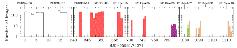
Figure 1: Histogram of the number of images per night collected during the four campaigns of our programme. The white histogram refers to observations in white light; the red, blue, green, and mango histograms refer to observations in the $R$, $B$, $V$, and $I$ filters, respectively.

All images of the OC M 67 [($\alpha,\delta$)=($08^{\rm h}51^{\rm m}18^{\rm s},+11^{\circ}48^{{}^{\prime}}00^{{}^{\prime\prime}}$)] were collected with the Asiago 67/92 cm Schmidt Telescope located on Mount Ekar (longitude $11.\!^{\circ}5710$ E, latitude $45.\!^{\circ}8430$ N, altitude 1370 m), that belongs to the Astronomical Observatory of Padova (OAPD), which is part of the Istituto Nazionale di Astrofisica (INAF). At the focus of the Schmidt telescope there is a SBIG STL-11000M camera, equipped with a Kodak KAI-11000M detector ($4050\times 2672$ pixel, field of view: $58\times 38$ arcmin², pixel scale: 862.5 mas pixel^-1). The characteristics of the telescope and the CCD are described in details in Paper I.

The OC M 67 is one of the four fields observed under the long-term observing programme APHN (PI: Bedin), aimed to characterise variable stars and transiting-exoplanet candidates in five OCs.

As in the case of M35 and NGC 2158 (Paper I), in the first observing season (2012) M 67 data were collected in white light (hereafter indicated with filter $N$, where $N$ stands for ’None’), with exposure time of 120 s, and 60 s (during the almost-full moon nights); during the second (2013) and the third season (2014) we collected 180 s+15 s $R$-filter and 180 s $B$-filter images. Finally, during the fourth season (2015), the observations were carried out in $I$-band (240 s+15 s) and $V$-band (240 s). In table 1 we give a log of the observations, while in Fig. 1 we show the histograms of the number of images taken during all the observing seasons.

All images are stored in the INAF national archive in Trieste.

Table 1: Log of observations.

Filter	# Images	Exp. Time	FWHM	Median FWHM
		(s)	(arcsec)	(arcsec)
$B$	57	$180$	1.20–1.86	1.47
$V$	13	$240$	1.59–2.31	1.90
$R$	588	$15$	1.33–7.66	3.17
	822	$180$
$I$	39	$15$	1.44–6.16	2.98
	78	$240$
$N$	232	$60$	1.70–7.38	3.41
	1878	$120$

For the data reduction, we used the software described in detail in Paper I. For each image we made a grid of $9\times 5$ spatially-varying, empirical point spread functions (PSFs), one for each of the 45 regions in which we divided the field of view (FOV); the software is similar to that developed by Anderson et al. (2006) for the Wide Field Imager (WFI) mounted at the ESO / Max-Planck-Gesellschaft (MPG) 2.2m telescope.

For any location on the detector, the best PSF model is obtained by a bilinear interpolation of the four closest PSFs and it is used to measure the position and the flux of the stars in each image.

We transformed stellar positions in all the images into the reference frame of the best image in filter $N$ (ID SC02906). For each filter, we obtained the photometric zero-points between the single images and the best image in that filter (ID: SC02906 for $N$-filter, SC37438 for $R$-filter, SC37437 for $B$-filter, SC46181 for $V$-filter, SC46722 for $I$-filter).

We created a stacked, high-signal-to-noise ratio (SNR) image (‘stack’) of the field for each filter. Using the $N$-filter stack, characterised by the highest SNR (Fig. 2), and the software used for single images, we derived an improved star list. We purged this star list from false detection using the qfit parameter (a diagnostic related to the quality of the PSF fit, Anderson et al. 2008) and the procedure described in Libralato et al. (2014). The purged star list contains 6905 sources, and we used it as the master star list (MSL) for the extraction of the light curves (LCs). The MSL contains stars with $V\lesssim 25$; faint enough to reach the magnitude of the faintest white dwarfs (WDs) detected along the cooling sequence of M 67 by Bellini et al. (2010b). The three bottom panels of Fig. 2 are centred on the three WDs shown in Fig. 2 of Bellini et al. (2010b). The bottom-right panel of Fig. 2 shows the faintest WD ($V\sim 24$) identified by the same authors. We extracted the $BVRI$-photometry of the 6905 sources in our catalogue by using the $BVRI$-stacked images. We calibrated the magnitudes by matching our catalogue to the Stetson Standard star catalogue (Stetson 2000). We derived calibration equations by means of least squares fitting of straight lines using magnitudes and colours.

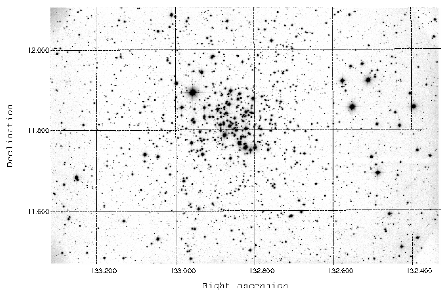
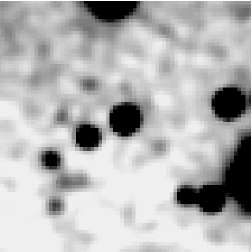
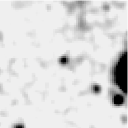
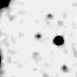
Figure 2: Top: $N$-filter stacked image of M 67 obtained with our data. Bottom: zoom-in of the $N$-filter stacked image centred on the three white dwarfs shown in Fig. 2 of Bellini et al. (2010b).

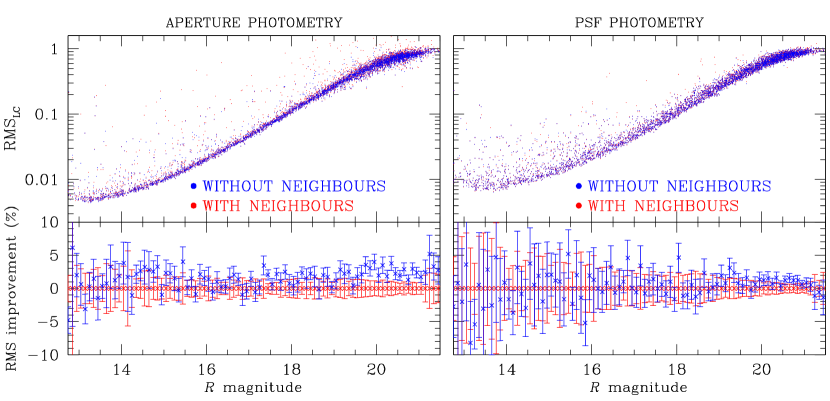
Figure 3: Photometric rms, obtained from original 180s $R$ images (red) and from images after neighbour-subtraction (blue), for both aperture photometry (left) and PSF photometry (right). The lower panels show the percentage improvement of the neighbour-subtraction algorithm on the rms, averaged over 0.1-mag bins.

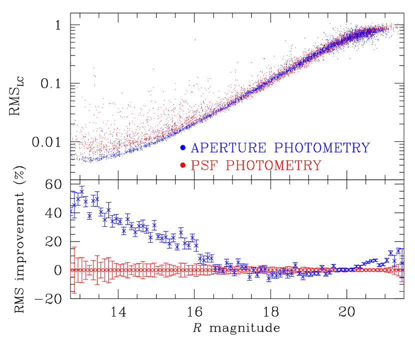
Figure 4: As in Fig. 3, but comparing aperture and PSF photometries on neighbour-subtracted images.

For the LCs extraction, we used the software developed and described in details in Paper I. Briefly, by using (i) the MSL catalogue, (ii) the PSFs, and (iii) the six-parameters linear transformations between the MSL and the single-image catalogues, for each target star within the MSL, the software extracts LCs in two parallel versions: a first one from the original images, and a second one from images where the neighbours close to the target star were PSF-fitted and subtracted. In both versions, our tool extracts the flux of the target star using PSF fitting and aperture photometry. As in Paper I, for aperture photometry we adopted a dynamical aperture that depends on the Full Width Half Maximum (FWHM), with radius $r$=$1.0\times{\rm FWHM}$. Therefore, for each star in the MSL, four light curves are generated: PSF with/without neighbour-subtracted and aperture with/without neighbour-subtracted.

In order to remove residual systematic errors from the LCs, we followed the procedure used in Paper I and described in detail in Nascimbeni et al. (2014). For each target star in each image, our algorithm computes local, weighted photometric zero-points using selected reference stars (generally the stars with the best rms at a given magnitude). The weights are a function of the relative on-sky position and of the magnitude difference between the target and the reference star. The software also computes a global zero-point correction, which —on average— provides worse residuals than the local zero-point correction, as also found in Paper I.

In Fig. 3 we show the photometric rms of the LCs derived from all the photometric methods (aperture with/without neighbours and PSF-fitting with/without neighbours). Even if the field of M 67 is relatively loose (if compared to the field analysed in Paper I) the photometry on images after neighbours subtraction is better than the photometry on original images, as the rms-scatter is lower and the rms-improvement is – on average – $\sim 3$% in the case of aperture photometry, and $\sim 1$% in the case of PSF-fitting photometry. Images were slightly de-focused to avoid saturation of main sequence (MS) turn off stars, therefore it was difficult to perfectly model the PSFs. This is also the reason why the rms PSF-fitting photometry is overall worse than the one associated to aperture photometry, as shown in Fig. 4.

3 Variable finding

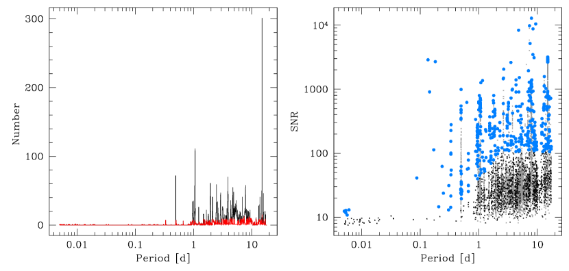
Figure 5: Procedure followed for the extraction of candidate variable stars. Left panel: distribution of the periods obtained from all the light curves before (black) and after (red) spikes suppression. Right panel:the AoV SNR as a function of the period of the light curves: in grey all the stars, in black the stars after spikes suppression, and in azure the suspected variables.

In order to detect candidate variables in our field, we used three different algorithms: the Generalized Lomb-Scargle (GLS) periodogram (Zechmeister & Kürster 2009), suitable for sinusoidal signals; the Analysis of Variance (AoV) periodogram (Schwarzenberg-Czerny 1989), useful to detect all variable types; the Box-fitting Least-Squares (BLS) periodogram (Kovács, Zucker & Mazeh 2002), effective for searching box-like dips in an otherwise flat or nearly flat LC, such as eclipsing binaries (EBs) and planetary transits. All the algorithms are part of the publicly available code VARTOOLS v.1.32 (Hartman et al. 2008). We used the output parameters associated to each algorithm for excluding the sources in our catalogue that have low probabilities to be variable in our data. In order to isolate the candidate variable stars, we used the procedure described in Paper I and summarised in Fig. 5.

From the histograms of the detected periods for all the LCs, we removed the spikes (saving the stars with high SNR, left panel of Fig. 5). The spikes are associated to spurious periods due to systematic effects, such as instrumental and atmospheric artefacts. In a second step, we selected by hand the candidate variables in the SNR versus period diagram (right panel of Fig. 5), and we visually inspected each of them.

We performed this procedure on neighbour-subtracted LCs, both for aperture and PSF photometries and for $N$ and $R$ LCs, identifying 68 real variable sources.

As in Paper I, we refined the periods using the following procedure: for each variable star, we normalised the $R$ and $N$ LC to zero, subtracting the 5$\sigma$-clipped median magnitude. Then, we merged the $R$ and $N$ normalised LCs, obtaining a LC with a temporal baseline of 764 days. We used again the VARTOOLS algorithms LS, AoV, and BLS to improve the period of the variable star. This procedure is useful only to improve the periods; it is not possible to extract any other scientific information from this normalised LC.

4 Variable stars and colour-magnitude diagrams

In our catalogue there are 6905 sources that cover a field-of-view of $\sim 0.612$ degree² centred on M 67. In this catalogue we find 68 variables stars. All the variable stars are listed in Table 2; for each variable we provide the identification number (ID), the position, the period (if it is not irregular), and, when available, the magnitudes in $NBVRIJ_{\rm 2MASS}H_{\rm 2MASS}K_{\rm 2MASS}$ bands, the membership probabilities as obtained in Sect. 4.1, and the radial velocities from Geller, Latham & Mathieu (2015).

Of these 68 variable stars, 25 variable stars have already been classified in other photometric works (Gilliland et al. 1991; Stassun et al. 2002; van den Berg et al. 2002; Sandquist & Shetrone 2003a, b; Stello et al. 2006, 2007; Bruntt et al. 2007; Pribulla et al. 2008; Yakut et al. 2009) and/or in the General Catalogue of Variable Stars (GCVS, Samus & Antipin 2013). Other variable stars listed in literature catalogues, but not found in our variable catalogue, are bright objects extremely saturated in our data (even in short exposures) or just outside the Schmidt FOV.

Table 2: First 10 lines of the catalogue of variable stars.

ID	$\alpha$	$\delta$	P	$N$	$B$	$V$	$R$	$I$	$J_{\rm 2MASS}$	$H_{\rm 2MASS}$	$K_{\rm 2MASS}$	$P_{\mu}$	RVa
	(degree)	(degree)	(day)									(%)	(km s-1)
(1)	(2)	(3)	(4)	(5)	(6)	(7)	(8)	(9)	(10)	(11)	(12)	(13)	(14)
10	132.48057	11.470550	6.61403975	-13.4283	15.6986	15.8312	14.8366	14.7724	13.665	13.276	13.262	90.5418	30.29
37	132.72530	11.480997	1.82830531	-10.526	20.3047	18.5991	17.7994	15.9833	14.631	13.999	13.724	2.3146	-1000.00
101	133.03346	11.503185	0.61441096	-9.9831	19.6606	18.757	18.0689	17.6468	16.401	15.96	15.59	14.8792	-1000.00
142	132.54111	11.514107	0.33958032	-9.3075	19.7992	19.3732	18.9384	18.9665	-99.999	-99.999	-99.999	44.9397	-1000.00
144	132.68428	11.515616	8.07609064	-13.5201	15.783	14.9577	14.7485	14.6447	13.572	13.167	13.079	0.347	55.34
193	133.08555	11.534070	5.01456608	-11.7733	17.9946	16.8831	16.339	15.7722	14.592	13.965	13.791	97.3684	-1000.00
207	133.09478	11.541483	10.8060368	-9.0553	-99.999	18.7736	18.9221	18.3115	16.559	15.826	15.243	49.6983	-1000.00
211	132.54888	11.540289	19.1807153	-14.0378	15.3067	14.4544	14.146	13.971	12.883	12.444	12.341	0.0	35.69
236	132.46906	11.551604	2.86317050	-16.0982	13.3535	12.4298	12.0711	11.9546	10.725	10.269	10.18	0.0	-15.61
239	132.55463	11.552562	6.75840156	-13.0745	16.1264	15.4163	15.1784	15.0959	14.076	13.766	13.733	0.0	13.22

Notes.   ^aGeller, Latham & Mathieu (2015).

4.1 Proper motions and membership probabilities

We used stellar proper motions to separate cluster members and field stars. The approach adopted to compute stellar positional displacement is the same as in many other works, e.g., Bedin et al. (2003); Anderson et al. (2006); Yadav et al. (2008); Bellini et al. (2010b); Nardiello et al. (2015b), and Libralato et al. (2015). Using six-parameter local transformations and a sample of likely cluster members (for example MS stars), we computed the displacement between the stellar positions in two different epochs, after been transformed into a common reference system. As first epoch, we used M 67 $V$-filter observations collected with the WFI mounted at the ESO/MPG 2.2 m telescope, on February 16th, 2000 ($t_{\rm I}$=2000.1). As second epoch we used the best 100 Schmidt $R$-images collected during the 2013 observational run ($t_{\rm II}\simeq$2013.1). The time baseline for the proper motion measurements is $\sim$13.0 yr.

Since we used likely cluster members to compute the coefficients of the six-parameter linear transformations, the stellar displacements are computed relative to the cluster mean motion. Therefore, by construction, the cluster distribution in the vector-point diagram (VPD) is centred around (0,0), while field stars, that have a different motion relative to that of the cluster, lie in a different region of the VPD (see Fig. 6).

The membership probabilities (MPs) of the stars in the M 67 FOV have already been calculated using both astrometry (e.g. Sanders 1977; Girard et al. 1989; Zhao et al. 1993; Yadav et al. 2008) and radial velocities (e.g Yadav et al. 2008; Pasquini et al. 2011; Geller, Latham & Mathieu 2015). Our final catalogue supplements the other works; we extracted the MPs in an homogeneous way for stars with $V\lesssim 19.5$ in a region of $58\times 38$ arcmin².

There are different methods to derive stellar MPs. We chose that described by Balaguer-Núnez, Tian & Zhao (1998). Briefly, we derived the frequency function for both cluster ($\Phi_{c}$) and field stars ($\Phi_{f}$). We assumed that cluster distribution is centred at ($\mu_{\alpha\cos\delta,c}$,$\mu_{\delta,c}$) $=$ (0.00,0.00) mas yr^-1 with an intrinsic dispersion of ($\sigma_{\mu_{\alpha\cos\delta,c}}$,$\sigma_{\mu_{\delta,c}}$) $=$ (0.65,0.71) mas yr^-1. For field stars, we have ($\mu_{\alpha\cos\delta,f}$,$\mu_{\delta,f}$) $=$ (9.34,$-$1.10) mas yr^-1 and a dispersion of ($\sigma_{\mu_{\alpha\cos\delta,f}}$,$\sigma_{\mu_{\delta,f}}$) $=$ (4.19,6.19) mas yr^-1. We ignored the spatial distribution of the two components and assumed that there is not a correlation between them (correlation coefficient $\gamma$ is set to 0). We excluded from our calculation poorly-measured-proper-motion stars. The membership probability is then computed as:

$$P_{\mu}=\frac{\Phi_{c}}{\Phi_{c}+\Phi_{f}}\,\,.$$

Panel (a) of Fig. 6 shows the available MPs $P_{\mu}$ as a function of the magnitude $V$. The figure shows that we measured reliable MPs for stars with $V\lesssim 19.5$.

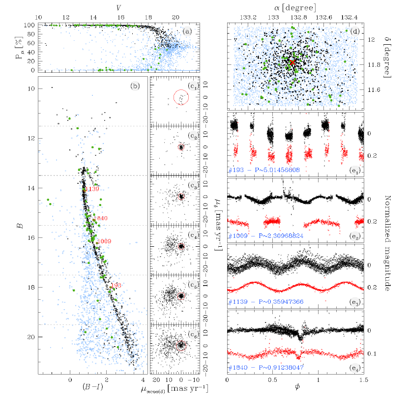
Figure 6: Panel (a): membership probabilities $P_{\mu}$ as a function of the $V$ magnitude; panel (b): CMD $B$ versus ($B-I$) of M 67 stars in the MSL; panels (c): vector-point diagrams for the same stars as in panel (b) in the corresponding magnitude intervals. The cluster star proper motion distribution is centred around (0,0) ; panel (d): positions ($\alpha$,$\delta$) for all the stars in the Schmidt MSL. The red cross indicates the cluster centre (Yadav et al. 2008); panels (e): four examples of median-magnitude normalised LCs in filter $N$ (black) and $R$ (red). The four stars have $P_{\mu}>97$%. In panels (a), (b), and (d), we plot in black the likely cluster members, i.e. the stars inside the red circles in panels (c), in azure the likely field stars, and in green the variable stars found in this work. In panel (b) we highlight the variable stars shown in panels (e).

4.2 Colour-magnitude diagrams and light curves

In panel (b) of Fig. 6 we show the $B$ versus $(B-I)$ CMD of M 67. In panels (a) and (b), we plot in black the likely cluster member stars, selected according to their proper motions (i.e. the stars inside the red circles in the VPD of panels c), in azure the stars rejected and those are likely field stars, and with green dots the variable stars found in this work. In panel (d), using the same colour-code, we plot the positions of the stars in our MSL field of view.

In panels (e) there are four examples of variable stars with $P_{\mu}>97$%. The LCs are normalised to the median magnitude. We plot in black the LC in $N$-filter and in red that in $R$-filter.

Panel (e₄) shows an eclipsing binary (ID #1840) that has never been photometrically observed, but that is in the sample of Geller, Latham & Mathieu (2015). From spectroscopic observations, they found that this is a double lined (SB2) eclipsing binary and also a X-ray source (X35 in the ROSAT catalogue, Belloni, Verbunt & Mathieu 1998). In our data, we probably observe only the primary eclipse, that has a box-like shape with a depth of 0.02 mag.

5 Electronic material

The catalogue of all the sources in our MSL is electronically available. The catalogue contains the following information: Cols (1) and (2) are the J2000.0 equatorial coordinates in decimal degrees; Cols (3) and (4) the positions in pixel on the $N$-filter stack; Cols (5)-(12) are the instrumental $N$, and the calibrated $BVRIJ_{\rm 2MASS}H_{\rm 2MASS}K_{\rm 2MASS}$ magnitudes (when the magnitude is not available, it is flagged with -99.999); Col. (13) is the identification number (ID) of the star; Cols. (14) and (15) give the relative proper motions in mas yr^-1 along ($\alpha\cos\delta,\delta$) direction (when it is not available, it is flagged with -999.9999); Col. (16) gives the membership probabilities $P_{\mu}$ (when it is not available, it is flagged with $-1$).

Along with the MSL, we release the catalogue of all variable stars found in this work. An example of the catalogue is Table 2: Col. (1) is the identification number (ID) of the variable star in our MSL; Cols (2) and (3) are the J2000.0 equatorial coordinates in decimal degree; Col. (4) contains the periods in day (when the star is irregular, the period is -99); Cols (5)-(12) are the instrumental $N$, and the calibrated $BVRIJ_{\rm 2MASS}H_{\rm 2MASS}K_{\rm 2MASS}$ magnitudes (when the magnitude is not available, it is flagged with -99.999); Col. (13) gives the membership probabilities $P_{\mu}$ (when it is not available, it is flagged with $-1$); Col. (14) are the radial velocities measured by Geller, Latham & Mathieu (2015) (when the radial velocity measurement is not available, it is denoted as -1000). For each variable star, we also release the $BRIN$ LCs.

Finally, we make the astrometrized stacks in $BVRIN$ filters electronically available.

6 Summary

In this work we present the photometric results for the third target (M 67) of the photometric survey of OC stars conducted with the 67/92 cm Schmidt telescope at Mount Ekar, Asiago. We analysed a total of 3707 images in $B$, $V$, $R$, $I$ and white light (no filter), collected over 3.1 years. We used the algorithms described in Nardiello et al. (2015a) to obtain a complete list of stars (6905 sources with magnitude $V\lesssim 25$) and to extract, detrend, and analyse the corresponding LCs. We identify 68 variable stars (43 of which are new). Combining Schmidt best data with WFI@2.2m MPG/ESO images (collected on 2000), we derived the relative proper motions and the membership probabilities for a great number of stars in our MSL. We release two electronic catalogues: the catalogue of variable stars, (containing coordinates, periods $B$, $V$, $R$, $I$, $N$, 2MASS magnitudes, membership probabilities, radial velocities) and the catalogue of all the sources in the Schmidt FOV (containing positions, $B$, $V$, $R$, $I$, $N$, 2MASS magnitudes, proper motions, membership probabilities). The electronic material includes the $B$, $V$, $R$, $I$, and white light stacked images and light curves of the identified variable stars.

The OC M 67 is in the field of the K2 Mission-Campaign-5. The released catalogue of M 67 sources will be an excellent input-list for the extraction of LCs from K2 images. In this sense, our survey is preparatory to the analysis of K2 data, and complements (and extends in time) the light curves of the stars covered by K2.

References

- Anderson et al. (2006) Anderson J., Bedin L. R., Piotto G., Yadav R. S., Bellini A., 2006, A&A, 454, 1029
- Anderson et al. (2008) Anderson J. et al., 2008, AJ, 135, 2114
- Balaguer-Núñez, Galadí-Enríquez & Jordi (2007) Balaguer-Núñez L., Galadí-Enríquez D., Jordi C., 2007, A&A, 470, 585
- Balaguer-Núnez, Tian & Zhao (1998) Balaguer-Núnez L., Tian K. P., Zhao J. L., 1998, A&AS, 133, 387
- Bedin et al. (2003) Bedin L. R., Piotto G., King I. R., Anderson J., 2003, AJ, 126, 247
- Bellini et al. (2010a) Bellini A., Bedin L. R., Pichardo B., Moreno E., Allen C., Piotto G., Anderson J., 2010a, A&A, 513, A51
- Bellini et al. (2010b) Bellini A. et al., 2010b, A&A, 513, A50
- Belloni, Verbunt & Mathieu (1998) Belloni T., Verbunt F., Mathieu R. D., 1998, A&A, 339, 431
- Brucalassi et al. (2014) Brucalassi A. et al., 2014, A&A, 561, L9
- Bruntt et al. (2007) Bruntt H. et al., 2007, MNRAS, 378, 1371
- Carraro et al. (1994) Carraro G., Chiosi C., Bressan A., Bertelli G., 1994, A&AS, 103, 375
- Demarque, Green & Guenther (1992) Demarque P., Green E. M., Guenther D. B., 1992, AJ, 103, 151
- Fan et al. (1996) Fan X. et al., 1996, AJ, 112, 628
- Geller, Latham & Mathieu (2015) Geller A. M., Latham D. W., Mathieu R. D., 2015, AJ, 150, 97
- Gilliland et al. (1991) Gilliland R. L. et al., 1991, AJ, 101, 541
- Girard et al. (1989) Girard T. M., Grundy W. M., Lopez C. E., van Altena W. F., 1989, AJ, 98, 227
- Grocholski & Sarajedini (2003) Grocholski A. J., Sarajedini A., 2003, MNRAS, 345, 1015
- Hartman et al. (2008) Hartman J. D., Gaudi B. S., Holman M. J., McLeod B. A., Stanek K. Z., Barranco J. A., Pinsonneault M. H., Kalirai J. S., 2008, ApJ, 675, 1254
- Howell et al. (2014) Howell S. B. et al., 2014, PASP, 126, 398
- Jacobson, Pilachowski & Friel (2011) Jacobson H. R., Pilachowski C. A., Friel E. D., 2011, AJ, 142, 59
- Janes & Smith (1984) Janes K. A., Smith G. H., 1984, AJ, 89, 487
- Kovács, Zucker & Mazeh (2002) Kovács G., Zucker S., Mazeh T., 2002, A&A, 391, 369
- Libralato et al. (2015) Libralato M. et al., 2015, MNRAS, 450, 1664
- Libralato et al. (2014) Libralato M., Bellini A., Bedin L. R., Piotto G., Platais I., Kissler-Patig M., Milone A. P., 2014, A&A, 563, A80
- Mathieu & Latham (1986) Mathieu R. D., Latham D. W., 1986, AJ, 92, 1364
- Mathieu, Latham & Griffin (1990) Mathieu R. D., Latham D. W., Griffin R. F., 1990, AJ, 100, 1859
- Mathieu et al. (1986) Mathieu R. D., Latham D. W., Griffin R. F., Gunn J. E., 1986, AJ, 92, 1100
- Milone (1992) Milone A. A. E., 1992, PASP, 104, 1268
- Milone & Latham (1994) Milone A. A. E., Latham D. W., 1994, AJ, 108, 1828
- Montgomery, Marschall & Janes (1993) Montgomery K. A., Marschall L. A., Janes K. A., 1993, AJ, 106, 181
- Nardiello et al. (2015a) Nardiello D. et al., 2015a, MNRAS, 447, 3536
- Nardiello et al. (2015b) Nardiello D., Milone A. P., Piotto G., Marino A. F., Bellini A., Cassisi S., 2015b, A&A, 573, A70
- Nascimbeni et al. (2014) Nascimbeni V. et al., 2014, MNRAS, 442, 2381
- Nissen, Twarog & Crawford (1987) Nissen P. E., Twarog B. A., Crawford D. L., 1987, AJ, 93, 634
- Pancino et al. (2010) Pancino E., Carrera R., Rossetti E., Gallart C., 2010, A&A, 511, A56
- Pasquini et al. (2008) Pasquini L., Biazzo K., Bonifacio P., Randich S., Bedin L. R., 2008, A&A, 489, 677
- Pasquini et al. (2012) Pasquini L. et al., 2012, A&A, 545, A139
- Pasquini et al. (2011) Pasquini L., Melo C., Chavero C., Dravins D., Ludwig H.-G., Bonifacio P., de La Reza R., 2011, A&A, 526, A127
- Pichardo et al. (2012) Pichardo B., Moreno E., Allen C., Bedin L. R., Bellini A., Pasquini L., 2012, AJ, 143, 73
- Pribulla et al. (2008) Pribulla T. et al., 2008, MNRAS, 391, 343
- Randich et al. (2006) Randich S., Sestito P., Primas F., Pallavicini R., Pasquini L., 2006, A&A, 450, 557
- Samus & Antipin (2013) Samus N. N., Antipin S. V., 2013, Astronomical and Astrophysical Transactions, 28, 49
- Sanders (1977) Sanders W. L., 1977, A&AS, 27, 89
- Sandquist (2004) Sandquist E. L., 2004, MNRAS, 347, 101
- Sandquist & Shetrone (2003a) Sandquist E. L., Shetrone M. D., 2003a, AJ, 126, 2954
- Sandquist & Shetrone (2003b) Sandquist E. L., Shetrone M. D., 2003b, AJ, 125, 2173
- Sarajedini, Dotter & Kirkpatrick (2009) Sarajedini A., Dotter A., Kirkpatrick A., 2009, ApJ, 698, 1872
- Schwarzenberg-Czerny (1989) Schwarzenberg-Czerny A., 1989, MNRAS, 241, 153
- Stassun et al. (2002) Stassun K. G., van den Berg M., Mathieu R. D., Verbunt F., 2002, A&A, 382, 899
- Stello et al. (2006) Stello D. et al., 2006, MNRAS, 373, 1141
- Stello et al. (2007) Stello D. et al., 2007, MNRAS, 377, 584
- Stetson (2000) Stetson P. B., 2000, PASP, 112, 925
- Taylor (2007) Taylor B. J., 2007, AJ, 133, 370
- van den Berg et al. (2002) van den Berg M., Stassun K. G., Verbunt F., Mathieu R. D., 2002, A&A, 382, 888
- VandenBerg & Stetson (2004) VandenBerg D. A., Stetson P. B., 2004, PASP, 116, 997
- Yadav et al. (2008) Yadav R. K. S. et al., 2008, A&A, 484, 609
- Yakut et al. (2009) Yakut K. et al., 2009, A&A, 503, 165
- Zechmeister & Kürster (2009) Zechmeister M., Kürster M., 2009, A&A, 496, 577
- Zhao et al. (1993) Zhao J. L., Tian K. P., Pan R. S., He Y. P., Shi H. M., 1993, A&AS, 100, 243