Explicit Densities of Multidimensional Lévy Walks

Abstract

We provide explicit formulas for asymptotic densities of the 2- and 3-dimensional ballistic Lévy walks. It turns out that in the 3D case the densities are given by elementary functions. The densities of the 2D Lévy walks are expressed in terms of hypergeometric functions and the right-side Riemann-Liouville fractional derivative which allows to efficiently evaluate them numerically. The theoretical results agree with Monte-Carlo simulations. The obtained functions solve certain differential equations with the fractional material derivative.

Lévy walks play an important role in statistical physics. For the first time they were analyzed in [18, 19] in the framework of generalized master equations. What distinguishes Lévy walks is a strong spatial-time coupling. Particles move at a constant velocity $v_{0}$ between turning points and choose a new direction at random [1, 8]. The time between each turn has a slowly decaying power-law tail $\psi(t)\propto t^{-1-\alpha}$ with $0<\alpha<1$, but the motion is ballistic [7]. These features cause that Lévy walks find many practical applications including bacteria swimming [9], blinking nanocrystals [3], light transport in optical materials [2] and human travel [20, 21]. For more we refer to [10], which is also a good introduction to the topic.

In the resent article [7] the shape of density profiles of 1-dimensional Lévy walks in the asymptotic long-time limit was found. However many observed phenomena are 2- or 3-dimensional [9] and up till now there were no methods of determining the probability density function (PDF) in this scenario. In this paper we solve this problem and introduce methods to find the explicit formulas for asymptotic PDFs both in 2- and 3-dimensional case. The 2D result is given by Eq. (1.12). The 3D result given by Eq. (2.4) has a particularly elegant and simple form. Moreover these PDFs solve certain differential equations [5] with the fractional material derivative [11, 12].

From mathematical point of view multidimensional Lévy walk is defined as [5]:

$$\mathbf{L}(t)=\sum_{i=1}^{N(t)}v_{0}T_{i}\mathbf{V}_{i}+\left(t-\sum_{i=1}^{N(t)}T_{i}\right)v_{0}\mathbf{V}_{N(t)+1},$$

where $N(t)=\max\{k\geq 0:\sum_{i=1}^{k}T_{i}\leq t\}$ is a renewal process, $T_{i}$ is a sequence of independent, identically distributed (IID) random variables with power-law distribution $\psi(t)\propto t^{-1-\alpha}$ governing time between turns and $\mathbf{V}_{i}$ is a sequence of IID random vectors governing a direction of the motion [1]. For simplicity we assume $v_{0}=1$.

In physical and mathematical literature appear also so-called wait-first Lévy walks and jump-first Lévy walks [10] defined as coupled continuous time random walks [6]. These processes have different properties, but the techniques presented here allow us to calculate the asymptotic PDF of these multidimensional processes as well.

Levy walk is rotationally invariant - each direction of the motion is equally possible. Therefore to determine the asymptotic PDF of $\mathbf{L}(t)$ it is enough to determine the asymptotic PDF of the radius $\left\|\mathbf{L}(t)\right\|$. In this work we use two main ideas. The first one concerns determining the asymptotic PDF of $L_{1}(t)$ - the projection of $\mathbf{L}(t)$ on the first axis. The second one is finding the relation between the distribution of $\left\|\mathbf{L}(t)\right\|$ and $L_{1}(t)$.

1 2D case

After each turn the particles choose the direction $\mathbf{V}_{i}$ randomly. We assume that each $\mathbf{V}_{i}$ has a uniform distribution on a circle. Let $G(\mathbf{x},t)$ denote the PDF of $\mathbf{L}(t)$, $\mathbf{x}=(x_{1},x_{2})\in\mathbb{R}^{2}$. In [5] authors found the limit process $\mathbf{X}(t)$ such that $n^{-1}\mathbf{L}(nt)\stackrel{{\scriptstyle n\rightarrow\infty}}{{\longrightarrow}}\mathbf{X}(t)$ in Skorokhod $J_{1}$ topology [14]. Calculating the PDF $H(\mathbf{x},t)$ of the limit process $\mathbf{X}(t)$ is equivalent to finding the desired asymptotic behavior of $G(\mathbf{x},t)$, that is a function $H(\mathbf{x},t)$ such that $G(\mathbf{x},t)\propto H(\mathbf{x},t)$. We know [5] that in the Fourier-Laplace transform space $H$ is given by

$$H(\mathbf{k},s)=\frac{1}{s}g\left(\frac{i\mathbf{k}}{s}\right)=\frac{1}{s}\frac{\int_{\mathbf{S}^{1}}\left(1-\left\langle\frac{i\mathbf{k}}{s},\mathbf{u}\right\rangle\right)^{\alpha-1}K(d\mathbf{u})}{\int_{\mathbf{S}^{1}}\left(1-\left\langle\frac{i\mathbf{k}}{s},\mathbf{u}\right\rangle\right)^{\alpha}K(d\mathbf{u})},$$

where $\mathbf{k}=(k_{1},k_{2})\in\mathbb{R}^{2}$ is the Fourier space variable, $s$ is the Laplace space variable, $K(d\mathbf{u})$ is a uniform distribution on a circle $\mathbf{S}^{1}$ and $\left\langle\;,\;\right\rangle$ denotes an inner product in $\mathbb{R}^{2}$. Now we can notice that $H_{1}(k_{1},s)=H((k_{1},0),s)$ gives us the Fourier-Laplace transform of PDF of $X_{1}(t)$ - the projection of $\mathbf{X}(t)$ on the first axis. A marginal distribution of the uniform distribution on a circle $K_{1}(d\mathbf{u})$ has the density [17]

$$K(du_{1})=\frac{1}{\pi}\frac{1}{\left(1-u_{1}^{2}\right)^{1/2}}du_{1},$$ (1.1)

thus $H_{1}(k_{1},s)=\frac{1}{s}g_{1}\left(\frac{ik_{1}}{s}\right),$ where

$$g_{1}(\xi)=\frac{\int_{-1}^{1}(1-\xi u)^{\alpha-1}\frac{1}{\pi\left(1-u^{2}\right)^{1/2}}du}{\int_{-1}^{1}(1-\xi u)^{\alpha}\frac{1}{\pi\left(1-u^{2}\right)^{1/2}}du}.$$ (1.2)

Since we are now dealing with a 1-dimensional process $X_{1}(t)$ we can use methods to invert the F-L transform from [7] which apply only to such processes. This gives us $H_{1}(x,t)=\frac{1}{t}\Phi_{1}\left(\frac{x}{t}\right),$ where

$$\Phi_{1}(x)=-\frac{1}{\pi}\lim_{\epsilon\rightarrow 0}\operatorname{Im}\left[\frac{1}{x+i\epsilon}g_{1}\left(-\frac{1}{x+i\epsilon}\right)\right].$$ (1.3)

After transformations we obtain

$$\Phi_{1}(x)=-\frac{1}{\pi x}\operatorname{Im}\frac{{}_{2}F_{1}((1-\alpha)/2,1-\alpha/2;1;\frac{1}{x^{2}})}{{}_{2}F_{1}(-\alpha/2,(1-\alpha)/2;1;\frac{1}{x^{2}})}$$ (1.4)

for $x\in(-1,1)$ and $\Phi_{1}(x)=0$ otherwise. Here ${}_{2}F_{1}(a,b;c;x)$ is a hypergeometrical function [13] defined as

$${}_{2}F_{1}(a,b;c;x)=\sum_{k=0}^{\infty}\frac{(a)_{k}(b)_{k}}{(c)_{k}}\frac{x^{k}}{k!}$$ (1.5)

for $|x|<1$ and analitacaly continued for $x>1$. In this series $(a)_{k}=\frac{\Gamma[a+k]}{\Gamma[a]}$ is the Pochhammer symbol. The hypergeometric functions can be evaluated numerically and are implemented in most of the mathematical packages including Matlab and Mathematica. Their use permits high-precision calculations.

We now relate the PDF $H_{R}(r,t)$ of the radius $\left\|\mathbf{X}(t)\right\|$ to the calculated the PDF of $X_{1}(t)$. The rotational invariance of Lévy walk $\mathbf{L}(t)$ implies the rotational invariance of the limit process $\mathbf{X}(t)$. Therefore to find $H(\mathbf{x},t)$ it suffices to determine $H_{R}(r,t)$. From $H(\mathbf{k},s)=\frac{1}{s}g\left(\frac{i\mathbf{k}}{s}\right)$ we deduce the scaling $H_{R}(r,t)=\frac{1}{t}\Phi_{R}\left(\frac{r}{t}\right)$. The factorisation of $\mathbf{X}(1)$ into radial and directional parts gives us

$$\mathbf{X}(1)\stackrel{{\scriptstyle d}}{{=}}\left\|\mathbf{X(1)}\right\|\mathbf{V},$$ (1.6)

where $\mathbf{V}$ is a random vector uniformly distributed on a circle, indepedent of $\left\|\mathbf{X(1)}\right\|$ and ”$\stackrel{{\scriptstyle d}}{{=}}$” denotes the equality of distribution. This implies

$$\mathbf{P}(|X_{1}(1)|\leq x)=\frac{2}{\pi}\int_{0}^{1}\frac{1}{(1-u^{2})^{1/2}}\mathbf{P}\left(\left\|\mathbf{X}(1)\right\|\leq\frac{x}{u}\right)du$$ (1.7)

for $x\geq 0$. The differentiation of the above equation yields

$$\Phi_{1}(x)=\frac{1}{\pi}\int_{0}^{1}\frac{1}{(1-u^{2})^{1/2}}\frac{1}{u}\Phi_{R}\left(\frac{x}{u}\right)du$$ (1.8)

and after some calculations we arrive at

$$\Phi_{R}(r)=-2\pi^{1/2}rD_{-}^{1/2}\{\Phi_{1}(x^{1/2})\}(r^{2}),$$ (1.9)

where $D_{-}^{1/2}$ is the right-side Riemann-Liouville fractional derivative of order $1/2$ [15]:

$$D_{-}^{1/2}\{f(x)\}(y)=-\frac{d}{dy}\frac{1}{\pi^{1/2}}\int_{y}^{\infty}\frac{f(x)}{(x-y)^{1/2}}dx.$$ (1.10)

This fractional derivative can be calculated numerically, for instance see [16] for Matlab code. Combining Eqs. (1.4) and (1.9) gives us

$$\Phi_{R}(r)=$$

$$\quad-\frac{2r}{\pi^{1/2}}D_{-}^{1/2}\Big{\{}\frac{1}{x^{1/2}}\operatorname{Im}\frac{{}_{2}F_{1}((1-\alpha)/2,1-\alpha/2;1;\frac{1}{x})}{{}_{2}F_{1}(-\alpha/2,(1-\alpha)/2;1;\frac{1}{x})}\Big{\}}(r^{2})$$

for $r\in(0,1)$. In Cartesian coordinates $H(\mathbf{x},t)$ can be calculated as

$$H(\mathbf{x},t)=\frac{1}{2\pi t\left\|\mathbf{x}\right\|}\Phi_{R}\left(\frac{\left\|\mathbf{x}\right\|}{t}\right).$$ (1.11)

Therefore

$$H(\mathbf{x},t)=-\frac{1}{\pi^{3/2}t^{2}}\times$$ (1.12)

$$\quad D_{-}^{1/2}\Big{\{}\frac{1}{x^{1/2}}\operatorname{Im}\frac{{}_{2}F_{1}((1-\alpha)/2,1-\alpha/2;1;\frac{1}{x})}{{}_{2}F_{1}(-\alpha/2,(1-\alpha)/2;1;\frac{1}{x})}\Big{\}}\left(\frac{\left\|\mathbf{x}\right\|^{2}}{t^{2}}\right)$$

for $\left\|\mathbf{x}\right\|<t$ and $H(\mathbf{x},t)=0$ in the opposite case. The right panel of FIG. 1 presents $H(\mathbf{x},1)$ for $\alpha=0.6$ calculated from Eq. (1.12). The result is in agreement with the density pictured in the left panel of FIG. 1 estimated using Monte Carlo (MC) methods from $10^{7}$ trajectories. The algorithm for simulating Lévy walks is presented in [4]. The drawback of using this algorithm is that it only gives the approximation of the asymptotic behavior of these processes. We observe that our Eq. (1.12) gives much more accurate results than MC methods. The right panel of FIG. 1 shows that $H(\mathbf{x},1)\rightarrow\infty$ when $\left\|\mathbf{x}\right\|\rightarrow 1$ and MC methods reveal it only after a large number of simulations which is time-consuming.

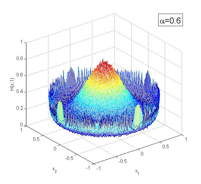
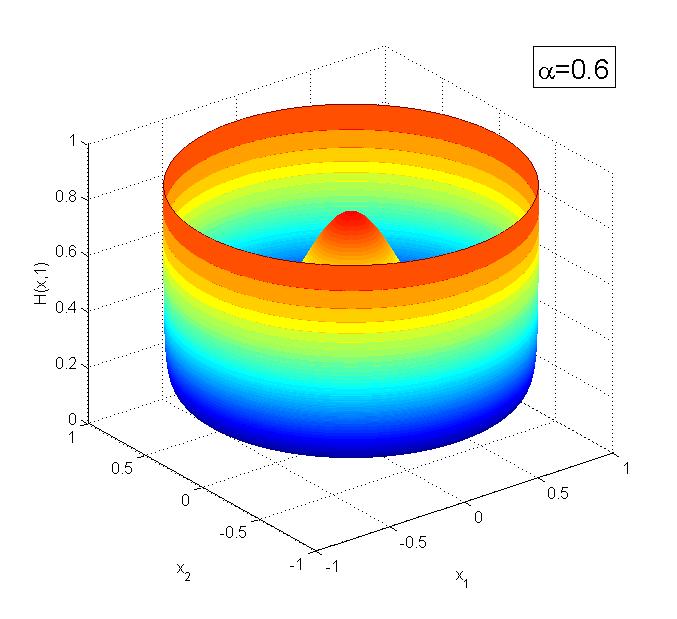
Figure 1: Density $H(\mathbf{x},1)$ of 2D Lévy walk with $\alpha 0.6$ estimated using Monte Carlo methods from $10^{7}$ trajectories (left) and obtained from Eq. (1.12) (right).

2 3D case

For 3D process $\mathbf{X}(t)=(X_{1}(t),X_{2}(t),X_{3}(t))$ we use similar methods. The notation remains the same. The random vectors $\mathbf{V}_{i}$ have a uniform distribution $K(d\mathbf{u})$ on a sphere $\mathbf{S}^{2}$. The Fourier-Laplace transform of $H(\mathbf{x},t)$ is (see [5])

$$H(\mathbf{k},s)=\frac{1}{s}\frac{\int_{\mathbf{S}^{2}}\left(1-\left\langle\frac{i\mathbf{k}}{s},\mathbf{u}\right\rangle\right)^{\alpha-1}K(d\mathbf{u})}{\int_{\mathbf{S}^{2}}\left(1-\left\langle\frac{i\mathbf{k}}{s},\mathbf{u}\right\rangle\right)^{\alpha}K(d\mathbf{u})},$$ (2.1)

where $\mathbf{k}=(k_{1},k_{2},k_{3})\in\mathbb{R}^{3}$ is the Fourier space variable, $s$ is the Laplace space variable and $\left\langle\;,\;\right\rangle$ denotes an inner product in $\mathbb{R}^{3}$. In the 3D case applying the same reasoning as in the 2D case yields simpler results. This is caused by the fact that a one dimensional marginal distribution $K_{1}(du_{1})$ of $K(d\mathbf{u})$ is uniform on the interval $[-1,1]$ (see [17]). Folowing the reasoning from the 2D case we obtain that the distribution of $X_{1}(1)$ is expressed by elementary functions

$$\Phi_{1}(x)=\frac{2(\alpha+1)}{\pi\alpha}\sin(\pi\alpha)\times$$

$$\quad\quad\quad\frac{(1-x^{2})^{\alpha}}{(1-x)^{2\alpha+2}+(1+x)^{2\alpha+2}+2\cos(\pi\alpha)(1-x^{2})^{\alpha+1}}$$

for $x\in(0,1)$, $\Phi_{1}(x)=\Phi_{1}(-x)$ for $x\in(-1,0)$ and $\Phi_{1}(x)=0$ otherwise. Equation (1.7) now has the form

$$\mathbf{P}(|X_{1}(1)|\leq x)=\int_{0}^{1}\mathbf{P}\left(\left\|\mathbf{X}(1)\right\|\leq\frac{x}{u}\right)du$$ (2.2)

and the following relation between $\Phi_{R}$ and $\Phi_{1}$ holds:

$$\Phi_{R}(r)=-2r\Phi_{1}^{\prime}(r).$$ (2.3)

Therefore

$$\Phi_{R}(r)=\frac{8}{\pi}\frac{\alpha+1}{\alpha}\sin(\pi\alpha)r(1-r^{2})^{\alpha-1}\times$$

$$\quad\quad\quad\quad\quad\frac{(1+r)^{2+2\alpha}(1+\alpha-r)-(1-r)^{2+2\alpha}(1+\alpha+r)-2r(1-r^{2})^{1+\alpha}\cos(\pi\alpha)}{\left((1+r)^{2+2\alpha}+(1-r)^{2+2\alpha}+2(1-r^{2})^{1+\alpha}\cos(\pi\alpha)\right)^{2}}$$ (2.4)

for $r\in(0,1)$ and $\Phi_{R}(r)=0$ in the opposite case. Figure 2 presents $\Phi_{R}(r)$ for different values of $\alpha$ calculated from Eq. (2.4). We notice that the theoretical results are in perfect agreement with the simulations. However contrary to using Eq. (2.4) the MC methods require a lot of time to get precise results.

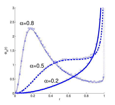
Figure 2: Density $\Phi_{R}(r)$ of 3D Lévy walk obtained from Eq. (2.4) for $\alpha=0.2$, $\alpha=0.5$ and $\alpha=0.8$ (lines). Theoretical results are compared with densities estimated using Monte Carlo methods (squares).

Concluding, in this Letter we derived the exact formulas for the asymptotic densities of the 2- and 3-dimensional ballistic Lévy walks. The result has a simple form, especially in the 3D case. The methods presented here can be successfully applied to different types of Lévy walks operating in a ballistic regime. Furthermore, the same techniques allow us to calculate the PDF of $n$-dimensional Lévy walks where the number of dimensions $n$ is arbitrary. We hope that these results will prove useful in practical applications.

^{1 2} Hugo Steinhaus Center,
Faculty of Pure and Applied Mathematics,
Wroclaw University of Technology,
Wyspianskiego 27, 50-370 Wroclaw, Poland.
¹ e-mail: marcin.magdziarz@pwr.edu.pl
² e-mail: tomasz.zorawik@pwr.edu.pl

References

- [1] J. Klafter, I.M. Sokolov, First Steps in Random Walks. From Tools to Applications. Oxford University Press, Oxford (2011)
- [2] P. Barthelemy, P.J. Bertolotti, D.S. Wiersma, A Lévy flight for light. Nature 453 (2008), 495–498.
- [3] G. Margolin, E. Barkai, Nonergodicity of blinking nanocrystals and other Lévy-walk processes. Phys. Rev. Lett. 94 (2005), 080601.
- [4] M. Magdziarz , M. Teuerle, Asymptotic properties and numerical simulation of multidimensional Lévy walks. Commun. Nonlinear Sci. Numer. Simul. 20 (2015), 489–505.
- [5] M. Magdziarz, H.P. Scheffler, P. Straka, P. Zebrowski (2015), Stoch. Proc. Appl.
- [6] E.W. Montroll and G.H. Weiss (1965) Random walks on lattices. II. J. Math. Phys. 6 , 167–181.
- [7] D. Froemberg, M. Schmiedeberg, E. Barkai, and V. Zaburdaev, Asymptotic densities of ballistic Lévy walks, Phys. Rev. E 91, 022131 (2015).
- [8] G. Zumofen and J. Klafter Phys. Rev. E 47, 851 (1993)
- [9] Gil Ariel, Amit Rabani, Sivan Benisty, Jonathan D. Partridge, Rasika M. Harshey, Avraham Be’er, Swarming bacteria migrate by Lévy Walk, Nature Communications 6 (2015).
- [10] V. Zaburdaev, S. Denisov, and J. Klafter, Lévy walks, Rev. Mod. Phys. 87, 483 (2015).
- [11] I.M. Sokolov, R. Metzler, Towards deterministic equations for Lévy walks: The fractional material derivative, Phys. Rev. E 67 (1) (2003) 1–4.
- [12] V V Uchaikin and R T Sibatov , Fractional Boltzmann equation for multiple scattering of resonance radiation in low-temperature plasma, 2011 J. Phys. A: Math. Theor. 44 145501.
- [13] Abramowitz, M. and Stegun, I. A. (Eds.). ”Hypergeometric Functions.” Ch. 15 in Handbook of Mathematical Functions with Formulas, Graphs, and Mathematical Tables, 9th printing. New York: Dover, pp. 555-566, 1972.
- [14] P. Billingsley, Convergence of Probability Measures, second ed., in: Wiley Series in Probability and Statistics, John Wiley & Sons Inc., New York, ISBN: 0471072427, 1968,
- [15] Kilbas A.A., Srivastava H.M., Trujillo J.J.: Theory and Applications of Fractional Differential Equations, North - Holland Mathematics Studies 204, Amsterdam (2006).
- [16] I. Podlubny, http://www.mathworks.com/matlabcentral/fileexchange/22071
- [17] Feller, W. An Introduction to Probability Theory and Its Applications, Vol. 2, 3rd ed. New York: Wiley, 1971.
- [18] M.F. Shlesinger, J. Klafter, Y.M Wong, Random walks with infinite spatial and temporal moments, J. Stat. Phys. 27 (1982), 499-512.
- [19] J. Klafter, A. Blumen, M.F. Shlesinger, Stochastic pathway to anomalous diffusion. Phys. Rev. A 35 (1987), 3081–3085.
- [20] D. Brockmann, L. Hufnagel, T. Geisel, The scaling laws of human travel. Nature 439 (2006), 462–465.
- [21] M.C. Gonzales, C.A. Hidalgo, A.L. Barabási, Understanding individual human mobility patterns. Nature 453(2008), 779–782.
1 2
Hugo Steinhaus Center,