PERCH: Perception via Search for
Multi-Object Recognition and Localization

Abstract

In many robotic domains such as flexible automated manufacturing or personal assistance, a fundamental perception task is that of identifying and localizing objects whose 3D models are known. Canonical approaches to this problem include discriminative methods that find correspondences between feature descriptors computed over the model and observed data. While these methods have been employed successfully, they can be unreliable when the feature descriptors fail to capture variations in observed data; a classic cause being occlusion. As a step towards deliberative reasoning, we present PERCH: PErception via SeaRCH, an algorithm that seeks to find the best explanation of the observed sensor data by hypothesizing possible scenes in a generative fashion. Our contributions are: i) formulating the multi-object recognition and localization task as an optimization problem over the space of hypothesized scenes, ii) exploiting structure in the optimization to cast it as a combinatorial search problem on what we call the Monotone Scene Generation Tree, and iii) leveraging parallelization and recent advances in multi-heuristic search in making combinatorial search tractable. We prove that our system can guaranteedly produce the best explanation of the scene under the chosen cost function, and validate our claims on real world RGB-D test data. Our experimental results show that we can identify and localize objects under heavy occlusion—cases where state-of-the-art methods struggle.

I Introduction

A ubiquitous robot perception task is that of identifying and localizing objects whose 3D models are known ahead of time: examples include robots operating in flexible automation factory settings, and domestic robots manipulating common household objects. Traditional methods for identifying and localizing objects rely on a two-step procedure: i) precompute a set of feature descriptors on the 3D models and match them to observed features, and ii) estimate the rigid transform between the set of found correspondences. In more recent methods, global descriptors jointly encoding object pose and viewpoint information are computed over different training instances, and a lookup is performed at test time. While such discriminative methods have been used successfully, they are limited by the ability of the feature descriptors to capture variations in observed data. For illustration, consider a scene with two objects, one almost completely occluding the other. Methods that employ feature correspondence matching fare poorly as key feature descriptors could be lost due to occlusion (Fig. 1), whereas learning-based methods could suffer as they might have not seen a similar training instance where the object is only partially visible.

We introduce an orthogonal approach to tackle this problem: Perception via Search (PERCH), which exploits the fact that the full 6 DoF sensor pose is available for most robotic systems. PERCH is a generative approach that attempts to simulate or render the scene which best explains the observed data. Our hypothesis is that if 3D models and sensor pose are available, we could perform deliberative reasoning: “under this configuration of objects in the scene for the given sensor pose, we would expect to see only this specific portion of that object”. The ability to reason deliberatively paves the way for an exhaustive search over possible configurations of objects.

While exhaustive search provides optimal solutions, it is often impractical owing to the size of the state space that grows exponentially with the number of objects in the scene. A key insight in this work is that the exhaustive search over possible scene configurations can be formulated as a tree search problem for a specific choice of an ‘explanation cost’. The formulation involves breaking down the scene explanation cost into additive components over individual objects in the scene, which in turn manifest as edge costs in a tree called the Monotone Scene Generation Tree. This allows us to use state-of-the-art heuristic search techniques for determining the configuration of objects that best explains the observed scene. We summarize our contributions below:

(a)

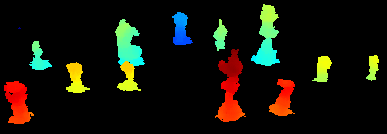
(b)

Figure 1: Identifying and localizing the pose of multiple objects simultaneously is challenging due to inter-object occlusions. 1 A scene showing multiple chess pieces occluding each other. 1 Top: The depth image from a Kinect sensor, colored by range. Bottom: The best-match depth image produced by our algorithm PERCH through searching over possible poses of the chess pieces.

• Perception via Search (PERCH), an algorithm for simultaneously localizing multiple objects in 2.5D or 3D sensor data when 3D models of those objects are available along with the camera pose.

• Formulating the multi-object localization problem as the minimization of an ‘explanation cost’ that captures the difference between the observed scene and the hypothesized scene.

• Exploiting structure in the explanation cost to cast it as a combinatorial search problem on a tree which we call the Monotone Scene Generation Tree. This alleviates the need to exhaustively generate/synthesize every possible scene while still returning solutions are that are provably optimal or bounded suboptimal.

• Incorporating parallelism in the search procedure, thereby allowing the algorithm to scale with the availability of computation.

In our experiments, we show how PERCH can localize objects even under heavy occlusion—a result which would be hard to obtain without explicit deliberative reasoning.

II Related Work

While model-based recognition and pose estimation of objects has been an active area of research for decades in the computer vision community [1, 2, 3], the proliferation of low-cost depth sensors such as the Microsoft Kinect has introduced a plethora of opportunities and challenges. We describe approaches in vogue for object recognition and localization from 3D sensor data, their limitations, inspirations from early research in vision that motivate our work, and the potential role of contemporary learning-based systems.

II-A Local and Global 3D Feature Descriptors

Model-based object recognition and localization in the present 3D era falls broadly under two approaches: local and global recognition systems. The former class of algorithms operate in a two step procedure: i) compute and find correspondences between a set of local shape-preserving 3D feature descriptors on the model and the observed scene and ii) estimate the rigid transform between a set of geometrically consistent correspondences. A final, optional and often used step is to perform a fine-grained local optimization to align the model to the scene and obtain the pose. Examples of local 3D feature descriptors range from Spin Images [4] to Fast Point Feature Histograms (FPFH) [5], whereas final alignment procedures include Iterative Closest Point (ICP) [6] and Bingham Procrustrean Alignment (BPA) [7]. The survey paper by Aldoma et al. [8] provides a comprehensive overview of other local approaches.

The second, global recognition systems employ a single-shot process for identifying object type and pose jointly. Global feature descriptors encode the notion of an object and capture shape and viewpoint information jointly in the descriptor. These approaches employ a training phase to build a library of global descriptors corresponding to different observed instances (e.g., each object viewed from different viewpoints) and attempt to match the descriptor computed at observation time to the closest one in the library. Additionally, global methods unlike the local ones, require points in the observed scene to be segmented into different clusters, so that descriptors can be computed on each object cluster separately. Some of the global recognition systems include Viewpoint Feature Histogram (VFH) [9], Clustered Viewpoint Feature Histogram (CVFH) [10], OUR-CVFH [11], Ensemble of Shape Functions (ESF) [12], and Global Radius-based Surface Descriptors (GRSD) [13]. Other approaches to estimating object pose include local voting schemes [14] or template matching [15] to first detect objects, and then using global descriptor matching or ICP for pose refinement.

Although both local and global feature-based approaches have enjoyed popularity owing to their speed and intuitive appeal, they suffer when used for identifying and localizing multiple objects in the scene. The limitation is perhaps best described by the following lines from the book by Stevens and Beveridge [16]: “Searching for individual objects in isolation precludes explicit reasoning about occlusion. Although the absence of a model feature can be detected (i.e., no corresponding data feature), the absence cannot be explained (why is there no corresponding data feature?). As the number of missing features increase, recognition performance degrades”. Global verification  [17, 18] and filtering [19] approaches somewhat attempt to address the occlusion problems faced by feature-based methods through a joint optimization procedure over candidate object poses, but are restricted by the fact that initial predictions for object poses are provided by a system that does not model occlusion. In this work, we aim to explicity reason about the interactions between multiple objects in the observed data by hypothesizing or rendering scenes, and using combinatorial search to control the number of scenes generated.

II-B Search and Rendering-based Approaches

The idea of using search to ‘explain’ scenes was popular in the early years of 2D computer vision: Goad [20] promoted the idea of treating feature matching between the observed scene and 3D model as a constrained search while Lowe [21] developed and implemented a viewpoint-constrained feature matching system. Grimson [22] introduced the Interpretation Tree to systematically search for geometrically-consistent matches between scene and model features, while using various heuristics to speed up search. Our work is also based on a search system, but it differs from the aforementioned works in that the search is over the space of full hypothesized/rendered scenes and not feature correspondences. In fact, our proposed algorithm does not employ feature descriptors at all.

The philosophy of the Render, Match and Refine (RMR) approach proposed by Stevens and Beveridge [23] motivates our work. RMR explicitly models interaction between objects by rendering the scene and uses occlusion data to inform measurement of similarity between the rendered and observed scenes. It then uses a global optimization procedure to iteratively improve the rendered scene to match the observed one. PERCH, our proposed algorithm, operates on a similar philosophy but differs in several details. The ‘explanation cost’ we use to compare the rendered and observed scene is based purely on 3D sensor data, as opposed to the 2D edge-feature and per-pixel depth differences used in RMR that make it vulnerable to offset errors between the rendered and observed 2D scenes. Moreover, the explanation cost we propose can be decomposed over the objects in the scene, thereby obviating the need for exhaustive search over the joint object poses.

Finally, an emerging trend for object recognition and pose estimation in RGB-D data is the use of deep neural networks trained on synthetic data generated using 3D models [24, 25]. As promising as deep learning methods are, they would require sufficient training data to capture invariances to multi-object interaction and occlusion, the generation of which is a combinatorial problem by itself. On the other hand, these methods could be incorporated in PERCH as heuristics for guiding deliberative search as discussed in Sec. IV-C.

III Problem Formulation

The problem we consider is that of localizing tabletop objects in a point cloud or 2.5D data such as from a Kinect sensor. The problem statement is as follows: given 3D models of $N$ unique objects, a point cloud ($I$) of a scene containing $K\geq N$ objects (possibly containing replicates of the $N$ unique objects), and the 6 DoF pose of the sensor, we are required to find the 3 DoF pose ($x,y,\theta$) of each of the $K$ objects in the scene.

We make the following assumptions:

• The number ($K$) and type of objects in the scene are known ahead of time (but not the correspondences themselves).

• The objects in the scene vary only in position $(x,y)$ and yaw $(\theta)$—3 DoF, with respect to their 3D models.

• The input point cloud can be preprocessed (table plane, background filtered etc.) such that the points in it only belong to objects of interest.

• We have access to the intrinsic parameters of the sensor, so that we can render scenes using the available 3D models.

We specifically note that we do not make any assumptions about the ability to ‘cluster’ points into different object groups as is done by most global 3D object recognition methods such as the Viewpoint Feature Histogram (VFH) [9].

III-A Notation

Throughout the paper, we will use the following notation:

• $O$: An object state characterized by $(\text{ID},x,y,\theta)$, the unique object ID, position and yaw.

• $I$: The input/observed point cloud from the depth sensor.

• $R_{j}$: A point cloud generated by rendering a scene containing objects $O_{1},O_{2},\ldots,O_{j}$.

• $p$: A point $(x,y,z)$ in any point cloud.

• $\Delta R_{j}=R_{j}-R_{j-1}$, the point cloud containing points in $R_{j}$ but not in $R_{j-1}$. In other words, the set of points belonging to object $O_{j}$ that would be visible given the presence of objects $O_{1},O_{2},\ldots,O_{j-1}$.

• $V(O_{j})$: The set of all points in the volume occupied by object $O_{j}$. When it is not possible to compute this in closed form, this can be replaced by an admissible/conservative approximation, for example, the volume of an inscribed cylinder.

• $V_{j}=\cup_{i=1}^{j}V(O_{i})$, the union of volumes occupied by objects $O_{1},O_{2},\ldots,O_{j}$.

III-B Explanation Cost Function

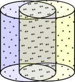
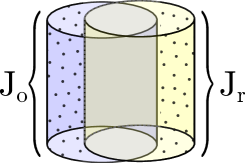
Figure 2: Illustration showing the computation of the explanation cost. The figure on the left shows the superposition of the observed point cloud (in blue) and the rendered point cloud (in yellow) of a cylindrical object. Object boundaries and volumes are shown merely for illustration. The total explanation cost (see figure on the right) is the number of unexplained points in the observed point cloud ($J_{o}$) and the number of unexplained points in the rendered point cloud ($J_{r}$).

We formulate the problem of identifying and obtaining the 3 DoF poses of objects $O_{1},O_{2},\ldots,O_{K}$ as that of finding the minimizer of the following ‘explanation cost’:

$$J(O_{1:K}) =J_{observed}(O_{1:K})+J_{rendered}(O_{1:K})$$

$$J_{observed}(O_{1:K}) =\sum_{p\in I}\mathds{1}_{[p\text{ is unexplained by }R_{K}]}$$

$$J_{rendered}(O_{1:K}) =\sum_{p\in R_{K}}\mathds{1}_{[p\text{ is unexplained by }I]}$$

in which the indicator function $\mathds{1}_{[p\text{ is unexplained by }C]}$ for a point cloud $C$ and point $p$ is defined as follows:

$$\mathds{1}_{[p\text{ is unexplained by }C]} =\begin{cases}1&\text{if }\min_{p^{\prime}\in C}\|p^{\prime}-p\|>\delta\\ 0&\text{otherwise}\end{cases}$$ (1)

for some sensor noise threshold $\delta$. We will use the notation $J_{o}$ and $J_{r}$ to refer to the observed and rendered explanation costs respectively.

The explanation cost essentially counts the number of points in the observed scene that are not explained by the rendered scene and the number of points in the rendered scene that cannot be explained by the observed scene. While it looks simplistic, the cost function forces the rendering of a scene that as closely explains the observed scene as possible, from both a ‘filled’ (occupied) and ‘empty’ (negative space) perspective. Figure 2 illustrates the computation of the ‘explanation cost’. Another interpretation for the explanation cost is to treat it as an approximation of the difference between the union volume and intersection volume of the objects in the observed and rendered scenes.

In the ideal scenario where there is no noise in the observed scene and where we have access to a perfect renderer, we could do an exhaustive search over the joint object poses to obtain a solution with zero cost. However, this naive approach is a recipe for computational disaster: even when we have only 3 objects in the scene and discretize our positions to 100 grid locations and 10 different orientations, we would have to synthesize/render $10^{9}$ scenes to find the global optimum. This immediately calls for a better optimization scheme, which we derive next.

IV PERCH: PErception via SeaRCH

IV-A Monotone Scene Generation Tree

The crux of our algorithm exploits the insight that the explanation cost function can be decomposed over the set of objects in the scene. To see this, we first note that the rendered scene containing $K$ objects, $R_{K}$ can be incrementally constructed:

$$R_{K} =\cup_{i=1}^{K}\Delta R_{i} \text{s.t. }R_{i-1}\subseteq R_{i}$$

where $\Delta R_{i}=R_{i}-R_{i-1}$ and $R_{0}$ is assumed to be an empty point cloud. The constraint $R_{i-1}\subseteq R_{i}$ translates to saying that the addition of a new object to the scene does not ‘occlude’ the existing scene, thereby guaranteeing that every point in $R_{i-1}$ exists in $R_{i}$ as well. In other words, the number of points in the rendered point cloud can only increase with the addition of a new object. The above constraint implicity assumes that the scene does not contain objects which can simultaneously occlude an object and also be occluded by another object, such as horseshoe-shaped objects. Using the above, we can write the rendered explanation cost as follows:

$$J_{r} =\sum_{p\in R_{K}}\mathds{1}_{[p\text{ is unexplained by }I]}$$

$$=\sum_{i=1}^{K}\sum_{p\in\Delta R_{i}}\mathds{1}_{[p\text{ is unexplained by }I]} \text{ s.t. }R_{i-1}\subseteq R_{i}$$

We then similarly decompose the observed explanation cost:

$$J_{o} =\sum_{p\in I}\mathds{1}_{[p\text{ is unexplained by }R_{K}]}$$

$$=\sum_{p\in I}\prod_{i=1}^{K}\mathds{1}_{[p\text{ is unexplained by }\Delta R_{i}]} \text{ s.t. }R_{i-1}\subseteq R_{i}$$

$$=\sum_{i=1}^{K}\sum_{p\in\{I\cap V(O_{i})\}}\mathds{1}_{[p\text{ is unexplained by }\Delta R_{i}]}$$

$$\;\qquad+\sum_{p\in\{I-V_{K}\}}\mathds{1}_{[p\text{ is unexplained by }R_{K}]} \text{ s.t. }R_{i-1}\subseteq R_{i}$$

With the above decompositions, we can re-write the overall optimization objective as:

$$J(O_{1:K}) =\sum_{i=1}^{K}\Delta J^{i} \text{ s.t. }R_{i-1}\subseteq R_{i}$$ (2)

$$=\sum_{i=1}^{K}\Delta J_{r}^{i}+\Delta J_{o}^{i} \text{ s.t. }R_{i-1}\subseteq R_{i}$$

where

$$\Delta J_{r}^{i} =\sum_{p\in\Delta R_{i}}\mathds{1}_{[p\text{ is unexplained by }I]}$$

$$\Delta J_{o}^{i} =\sum_{p\in\{I\cap V(O_{i})\}}\mathds{1}_{[p\text{ is unexplained by }\Delta R_{i}]}+\text{residual}(i)$$

$$\text{residual}(i) =\begin{cases}\sum_{p\in\{I-V_{K}\}}\mathds{1}_{[p\text{ is unexplained by }R_{K}]}&\text{ if }i=K\\ 0&\text{ otherwise }\end{cases}$$

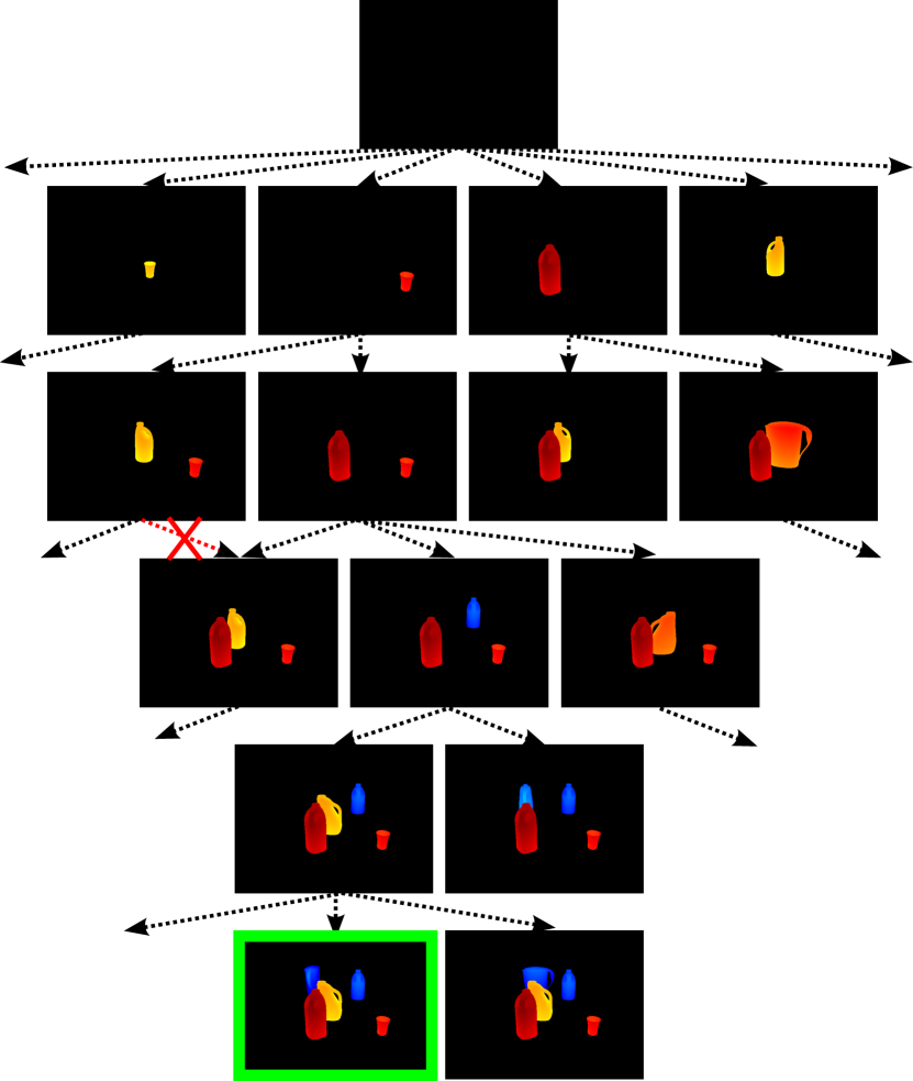
Figure 3: Portion of a Monotone Scene Generation Tree (MSGT): the root of the tree is the empty scene, and new objects are added progressively as we traverse down the tree. Notice how child states never introduce an object that occludes objects already in the parent state. A counter-example (marked by the red cross) is also shown. Any state on the $K^{\text{th}}$ level of the tree is a goal state, and the task is to find the one that has the lowest cost path from the root—marked by a green bounding box in this example.

Figure 4: A subset of all the states ‘generated’ during the tree search for the scene in Fig. 3. This figure is best viewed with digital zoom.

Equation 2 defines a pairwise-constrained optimization problem, the constraint being that the assignment of the $i^{\text{th}}$ object does not occlude the scene generated by the assignment of the previous objects $1$ through $i-1$. A natural way to solve this problem is to construct a tree that satisifies the required constraint, and assigns the object poses in a sequential order. This is precisely our approach and the resulting tree we construct is called the Monotone Scene Generation Tree (MSGT), with ‘monotone’ emphasizing that as we go down the tree, newly added objects cannot occlude the scene generated thus far (Fig. 3). We note that while a particular configuration of objects can be generated by choosing different assignment orders, only one is sufficient to retain as all those configurations have identical explanation costs. Thus, we obtain a tree structure instead of a Directed Acyclic Graph (DAG). Formally, any vertex/state in the MSGT is a partial assignment of object states: $s=\{O_{1:j}\}$, with $j\leq K$. For a MSGT state $s$ with an assignment of $j$ objects, the implicit successor generation function and the associated cost are defined as follows:

$$\textsc{Succ}(s) =\{s^{\prime}|s^{\prime}=s\cup O_{j+1}\land R_{j}\subseteq R_{j+1}\}$$ (3)

$$\textsc{c}(s,s^{\prime}) =\Delta J^{j+1}=\Delta J_{r}^{j+1}+\Delta J_{o}^{j+1}$$ (4)

The root node of the tree $s_{\text{root}}$ is an empty state containing no object assignments, while a goal state is any state $s$ that has an assignment for all objects. Given the MSGT construction, the multi-object localization problem reduces to that of finding the cheapest cost path in the tree from the root state to any goal state.

IV-B Tree Search

Although we have replaced exhaustive search with tree search, the problem still remains daunting owing to its branching factor. Assume that we have $d$ possible configurations $(x,y,\theta)$ for each object. Then, the worst case branching factor for the MSGT is $d^{K}$ for all levels if we allow repetition of objects in the scene, or $d^{K-i}$ for level $i$ if there is no repetition. Figure 4 illustrates this by showing a subset of the states generated during the tree search corresponding to the scene in Fig. 3. While heuristic search techniques such as A* are often a good choice for such problems, they require an admissible heuristic that provides a conservative estimate of the remaining cost-to-go. Usual heuristic search methods are limited by the following: i) admissible heuristics are non-trivial to obtain for this problem, and ii) they cannot support multiple heuristics, each of which could be useful on their own—for e.g, different feature-based and learning-based methods could serve as a heuristic each. Fortunately, recent work in heuristic search [26, 27] allows us to use multiple, inadmissible heuristics to find solutions with bounded suboptimality guarantees.

The particular multi-heuristic search we use is the Focal-MHA* [26] algorithm, and its choice is motivated by the fact that it permits the use of inadmissible heuristics that have no connection with the cost structure of the problem. This necessity will become clear in Sec. IV-C. At a high level, Focal-MHA* operates much like A* search. Like A*, it maintains a priority list of states ordered by an estimate of the path cost through that state and repeatedly ‘expands’ the most promising states until a goal is found. The difference from A* is in that Focal-MHA* interleaves this process with expansion of states chosen greedily by other heuristics [26]. Finally, Focal-MHA* guarantees that the solution found will have a cost which is bounded by $w\cdot\text{OPT}$, where OPT is the optimal solution cost and $w(\geq 1)$ is a user-chosen suboptimality bound. Algorithm 1 shows an instantiation of Focal-MHA* in the context of PERCH.

Algorithm 1 PERCH

The implicit MSGT construction (Eq. 3 and Eq. 4).

Suboptimality bound factor $w$ ($\geq 1$).

$1$ admissible heuristic $h$ and $n$ arbitrary, possibly inadmissible, heuristics $h_{1},h_{2},\ldots,h_{n}$.

An assignment of object poses $s_{\text{goal}}$ with $|s_{\text{goal}}|=K$ whose cost is within $w\cdot\text{OPT}$.

1:procedure Main()

2:    $s_{\text{root}}\leftarrow\{\}$

3:    planner $\leftarrow$ Focal-MHA*-Planner()

4:    planner.$\textsc{SetImplicitTree}(\textsc{Succ}(s),c(s,s^{\prime}))$

5:    planner.$\textsc{SetSuboptimalityFactor}(w)$

6:    planner.$\textsc{SetStartState}(s_{\text{root}})$

7:    planner.$\textsc{SetHeuristics}(h,h_{1},\ldots,h_{n})$

8:    planner.$\textsc{SetGoalCondition}(\text{\bf{return true} if }|s|=K)$

9:    $\{s_{\text{root}},s_{1},s_{2},\ldots,s_{\text{goal}}\}\leftarrow$ planner.$\textsc{ComputePath}()$

10:    return $s_{\text{goal}}$

IV-C Heuristics

Focal-MHA* requires one admissible and multiple inadmissible heuristics. Constructing an informative admissible heuristic is non-trivial for this setting, and thus we set our admissible heuristic to the trivial heuristic that returns $0$ for all states. We next describe our inadmissible heuristics.

The large branching factor of the MSGT might result in the search ‘expanding’ or opening every node in a level before moving on to the next. To guide the search towards the goal, a natural heuristic would be a depth-first heuristic that encourages expansion of states further down in the tree. Consquently, our first inadmissible heuristic for Focal-MHA* is the depth heuristic that returns the number of assignments left to make:

$$h_{depth}(s)=K-|s|$$

As a reminder, states with smaller heuristic values are expanded ahead of those with larger values. Next, it would be useful to encourage the search to expand states that have maximum overlap with the observed point cloud $I$ so far, rather than states with little overlap with the observed scene. Our second heuristic is therefore the overlap heuristic that counts the number of points in $I$ that do not fall within the volume of assigned objects:

$$h_{overlap}(s)=|I|-\sum_{p\in I}\mathds{1}_{[p\in V_{j}]}$$

where $j=|s|$ and $V_{j}$ is the union of the volumes occupied by the $j$ assigned objects. Another interpretation for this heuristic is the number of points in the observed scene that are outside the space carved by objects assigned thus far.

While we use only the above two heuristics in this work, we note that there is a possibility of using a wide class of heuristics derived from feature and learning-based methods. For instance, if an algorithm like VFH [9] produced a pose estimate $O_{j}^{\prime},j=1,2,\ldots,K$ for each of the $K$ objects in the scene, then a heuristic for $s$ with $|s|=j$ could resemble $\sum_{i=1}^{j}\|O_{i}-O_{i}^{\prime}\|$ for some appropriate choice of the norm. More generally, the multi-heuristic approach we use provides a framework to plug in various discriminative algorithms each with their own strengths and weaknesses.

IV-D Theoretical Properties

PERCH inherits all the theoretical properties of Focal-MHA* [26]. We state those here without proof:

Theorem 1

PERCH is complete with respect to the construction of the graph, i.e, if a solution (feasible assignment of all object poses) exists in the MSGT, it will be found.

Theorem 2

The returned solution has an explanation cost which is no more than $w$ times the cost of the best possible solution under the chosen graph construction.

As a disclaimer, we note that bounded suboptimal solutions with regard to the explanation cost do not translate to any bounded suboptimal properties with respect to the true object poses in the observed scene.

IV-E Implementation Details

IV-E1 Compensating for Discretization

The most computationally complex part of PERCH is that of generating successor states for a given state in the MSGT. This involves generating and rendering every state that contains one more object than the number in the present state, in every possible configuration. Several elements influence this branching factor: the number of objects in the scene, the chosen discretization for object poses, whether objects are rotationally symmetric (in which case only $(x,y)$ is of interest) etc. In our implementation, we limit the complexity by favoring coarse discretization and compensating with a local alignment technique such as ICP [6]. Specifically, every time we render a state with a new object, we take the non-occluded portion and perform an ICP alignment in the local vicinity of the observed point cloud. This allows us to obtain accurate pose estimates while retaining a coarse discretization. We do note that the underlying MSGT now becomes a function of the observed point cloud due to the ICP adjustment.

IV-E2 Parallelization

The generation of successor states is an embarassingly parallel process. We exploit this in our implementation by using multiple processes to generate successors in parallel. Theoretically, with sufficient number of cores, the time to expand a state would simply be the time to render a single scene.

V Experiments

V-A Occlusion Dataset

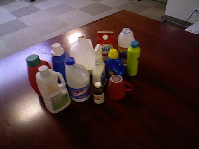
(a)

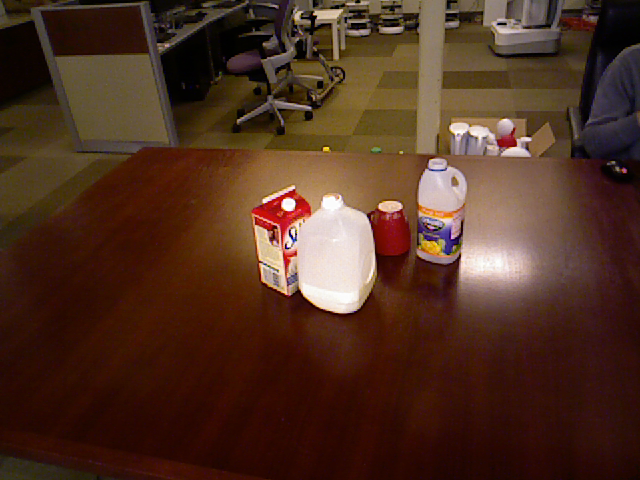
(b)

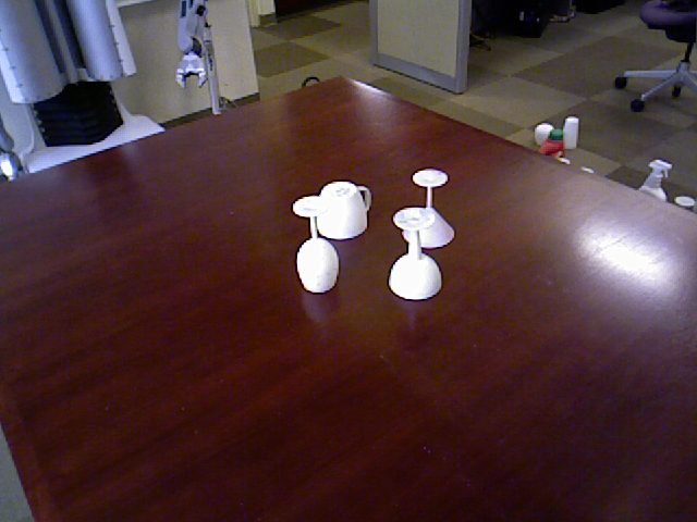
(c)

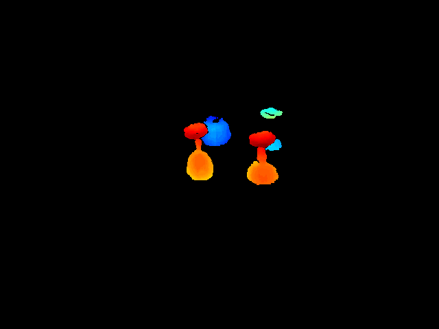
(d)

Figure 5: 5(a) A subset of the objects in the RGB-D occlusion dataset. 5(b) An example scene from the dataset. 5(c) Another example from the dataset and 5(d) the corresponding depth image (mapped to jet color) obtained after preprocessing. In this example, portion of the occluded glass is missing due to sensor noise, making it challenging for methods that rely on segmenting the scene into cohesive object point clouds.

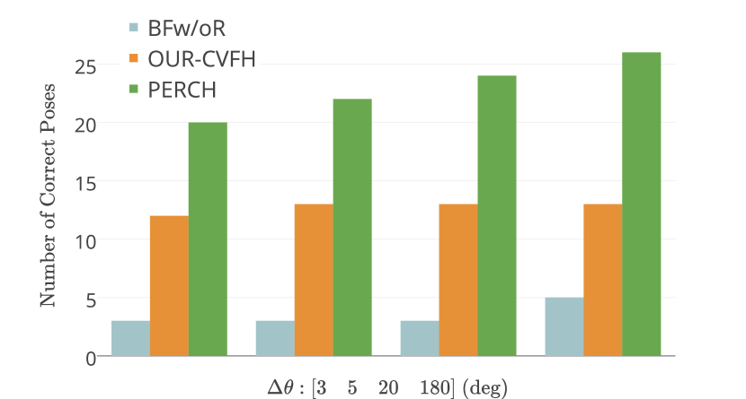
(a) $\Delta t=0.01m$

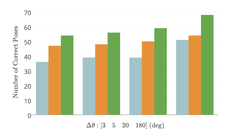
(b) $\Delta t=0.05m$

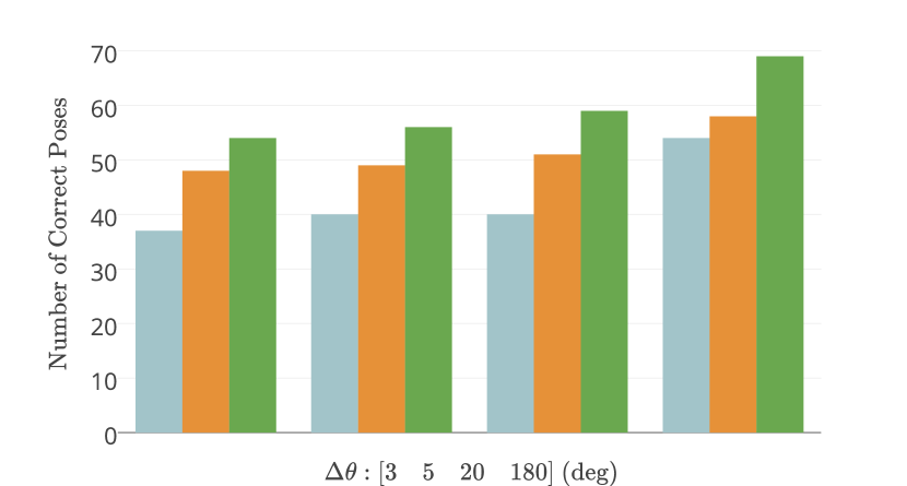
(c) $\Delta t=0.1m$

Figure 6: Number of objects whose poses were correctly classified by the baseline methods (BFw/oR, OUR-CVFH) and PERCH, for different definitions of ‘correct pose’.

To evaluate the performance of PERCH for multi-object recognition and pose estimation in challenging scenarios where objects could be occluding each other, we pick the occlusion dataset described by Aldoma et al. [8] that contains objects partially touching and occluding each other. The dataset contains 3D CAD models of 36 common household objects, and 23 RGB-D tabletop scenes with 82 object instances in total. All scenes except one contain objects only varying in translation and yaw, with some objects flipped up-side down. Since PERCH is designed only for 3D pose estimation, we drop the one non-compatible scene from the dataset, and preprocess the 3D CAD models such that they vary only in translation and yaw with respect to the ground truth poses. Figure 5 shows some examples from the dataset.

V-B PERCH Setup

Since PERCH requires that points in the scene only belong to objects of interest, we first preprocess the scene to remove the tabletop and background. Then, based on the RANSAC-estimated table plane, we compute a transform that aligns the point cloud from the camera frame to a gravity aligned frame, to simplify construction of the MSGT. PERCH has two parameters to set: the sensor noise threshold $\delta$ for determining whether a point is ‘explained’ (Eq. 1), and the suboptimality factor $w$ for the Focal-MHA* algorithm. In our experiments, we set $\delta$ to $3$ mm to account for uncertainty in the depth measurement from the Kinect sensor, as well as inaccuracies in estimating the table height using RANSAC. For the suboptimality factor $w$, we use a value of $3$. While this results in solutions that can be suboptimal by a factor of upto $3$, it greatly speeds up the search since computing the optimal solution typically takes much more time [28]. For Focal-MHA*, we use the two heuristics described in Sec. IV-C. Finally, for defining the MSGT we pick a discretization resolution of $4$ cm for both $x$ and $y$ and $22.5$ degrees for yaw. The adaptive ICP alignment (Sec. IV-E1) is constrained to find correspondences within $2$ cm, which is half the discretization resolution.

V-C Baselines

Our first baseline is the OUR-CVFH global descriptor [11], a state-of-the-art global descriptor designed to be robust to occlusions. By clustering object surfaces into separate smooth regions and computing descriptors for each portion, OUR-CVFH can handle occlusions better than descriptors such VFH and FPFH. Furthermore, it has the added advantage of directly encoding the full pose of the object, with no ambiguity in camera roll. We build the training database by rendering 642 views of every 3D CAD model from viewpoints sampled around the object. Then, for computing the training descriptors we use moving least squares to upsample every training view to a common resolution followed by downsampling to the Kinect resolution of $3$ mm as suggested in the OUR-CVFH paper [11]. Since the number and type of models in the test scene is assumed to be known for PERCH, we use the following pipeline for fair comparison: for the $K$ largest clusters in the test scene we obtain the histogram distance to each of the models we know that are in the scene. Then, we solve a min-cost matching problem to assign a particular model (and associated pose) to each cluster and obtain a feasible solution. Finally, we constrain the full 6 DoF poses returned by OUR-CVFH to vary only in translation and yaw and perform a local ICP alignment for each object pose.

The second baseline is an ICP-based optimization one, which we will refer to as Brute Force without Rendering (BFw/oR). Here, we slide the 3D model of every object in the scene over the observed point cloud (at the same discretization used for PERCH), and perform a local ICP-alignment at every step. The location ($x,y,\theta)$ that has the best ICP fitness score is chosen as the final pose for that model and made unavailable for other objects that have not yet been considered. Since the order in which the models are chosen for sliding can influence the solution, we try all permutations of the ordering ($K!$) and take the overall best solution based on the total ICP fitness score.

V-D Evaluation

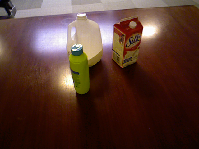
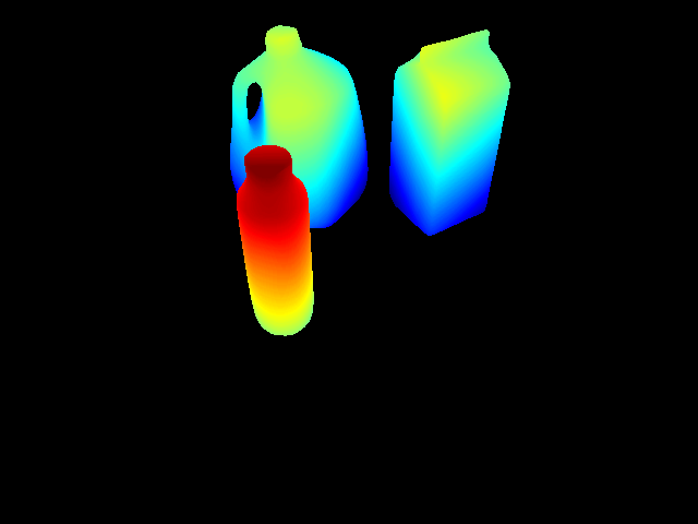
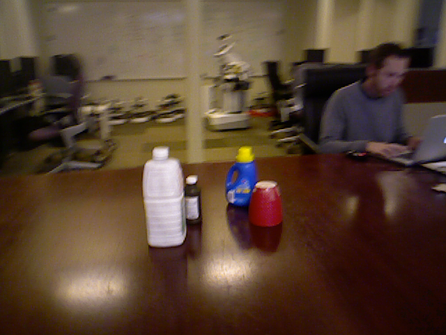
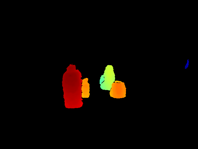
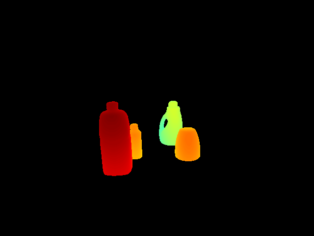
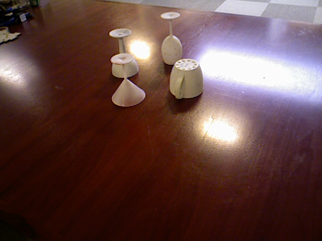
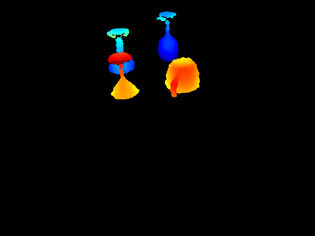
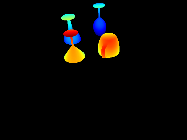
Figure 7: Examples showing the output of PERCH on the occlusion dataset. Left: RGB-D scenes in the dataset. Middle: Depth images of the corresponding input RGB-D scenes, Right: The depth image reconstructed by PERCH through rendering object poses.

To evaluate the accuracy of object localization, we use the following criterion: a predicted pose $(x,y,\theta)$ for an object is considered correct if $\|(x,y)-(x_{\text{true}},y_{\text{true}})\|_{2}<\Delta t$ and $\textsc{ShortestAngularDifference}(\theta,\theta_{\text{true}})<\Delta\theta$. We then compute the number of correct poses produced by each method for different combinations of $\Delta t$ and $\Delta\theta$. Figure 6 compares the performance of PERCH with BFw/oR and OUR-CVFH. Immediately obvious is the significant performance of PERCH over the baseline methods for $\Delta t=0.01m$. PERCH is able to correctly estimate the pose of over 20 objects with translation error under $1$ cm and rotation error under $5$ degrees. While the baseline methods have comparable recall for higher thresholds, they are unable to provide as many precise poses as PERCH does. Further, PERCH consistently dominates the baseline methods for all definition of ‘correct pose’. Among all methods, BFw/oR performs the worst. This is mainly due to the fact that it uses the point cloud corresponding to the complete object model for ICP refinement, rather than the point cloud corresponding to the unoccluded portion of the object. Again, this showcases the necessity to explicity reason about self-occlusions as well as inter-object occlusions.

The last column of the histogram in Fig. 6(c) (corresponding to $\Delta t=0.1$, $\Delta\theta=180$) is essentially a measure of recognition alone—PERCH can correctly identify 69 of the 80 object instances, where ‘identified’ is defined as obtaining a translation error under $10$ cm. Figure 7 shows some qualitative examples of PERCH’s peformance on the occlusion dataset. Further examples and illustrations are provided in the supplementary video.

V-E Computation Time and Scalability

Unlike global descriptor approaches such as OUR-CVFH which require an elaborate training phase to build a histogram library, PERCH does not require any precomputation. Consequently, the run time cost is high owing to the numerous scenes that need to be rendered. However, as mentioned earlier, the parallel nature of the problem and the easy availability of cluster computing makes this less daunting. For our experiments, we used the MPI framework to parallelize the implementation and ran the tests on a cluster of 2 Amazon AWS m4.10x machines, each having a 40-core virtual CPU. For each scene, we used a maximum time limit of 15 minutes and took the best solution obtained within that time. Overall, the mean planning time was 6.5 minutes, and the mean number of hypotheses rendered (i.e, states generated) was 15564.

Finally, to demonstrate that PERCH can be used for scenes containing several objects, we conducted a test on a chessboard scene (Fig. 1). We captured a Kinect depth image of the scene containing 12 pieces, of which 6 are unique and 4 are rotationally symmetric. We ran PERCH with suboptimality bound factor $w=15$ and sensor resolution $\delta=7.5$ mm, and took the best solution found within a time limit of 20 minutes. The solution found (i.e., the depth image corresponding to the goal state) is shown in Fig. 1.

VI Conclusions

In his lecture on computer heuristics in 1985 [29], Richard Feynman notes that if one had access to all the generative parameters of a scene (lighting, model etc.), one could possibly generate every single scene and take the best match to the observed data. We presented PERCH as a first step towards this deliberative reasoning. The key contributions were the formulation of multi-object recognition and localization as an optimization problem and designing an efficient combinatorial search algorithm for the same. We demonstrated how PERCH can robustly localize objects under occlusion, and handle scenes containing several objects.

While our results look promising on the accuracy front, much work remains to be done in making the algorithm suitable for real-time use. Our future work involves exploring optimizations and heuristics for the search to obtain faster yet high quality solutions. Specifically, we are interested in leveraging state-of-the-art discriminative learning to provide guidance for the search. Other directions include generalizing PERCH to a variety of perception tasks that require deliberative reasoning.

References

- Roberts [1963] L. G. Roberts, “Machine perception of three-dimensional solids,” Ph.D. dissertation, Massachusetts Institute of Technology, 1963.
- Brooks [1981] R. A. Brooks, “Symbolic reasoning among 3-d models and 2-d images,” Artificial intelligence, vol. 17, no. 1, pp. 285–348, 1981.
- Lowe [1987a] D. G. Lowe, “Three-dimensional object recognition from single two-dimensional images,” Artificial intelligence, vol. 31, no. 3, pp. 355–395, 1987.
- Johnson and Hebert [1999] A. E. Johnson and M. Hebert, “Using spin images for efficient object recognition in cluttered 3d scenes,” Pattern Analysis and Machine Intelligence, IEEE Transactions on, vol. 21, no. 5, pp. 433–449, 1999.
- Rusu et al. [2009] R. B. Rusu, N. Blodow, and M. Beetz, “Fast point feature histograms (fpfh) for 3d registration,” in ICRA. IEEE, 2009, pp. 3212–3217.
- Chen and Medioni [1991] Y. Chen and G. Medioni, “Object modeling by registration of multiple range images,” in Robotics and Automation, 1991. Proceedings., 1991 IEEE International Conference on. IEEE, 1991, pp. 2724–2729.
- Glover and Popovic [2013] J. Glover and S. Popovic, “Bingham procrustean alignment for object detection in clutter,” in IROS. IEEE, 2013, pp. 2158–2165.
- Aldoma et al. [2012a] A. Aldoma, Z.-C. Marton, F. Tombari, W. Wohlkinger, C. Potthast, B. Zeisl, R. B. Rusu, S. Gedikli, and M. Vincze, “Point cloud library,” IEEE Robotics & Automation Magazine, vol. 1070, no. 9932/12, 2012.
- Rusu et al. [2010] R. B. Rusu, G. Bradski, R. Thibaux, and J. Hsu, “Fast 3d recognition and pose using the viewpoint feature histogram,” in IROS. IEEE, 2010, pp. 2155–2162.
- Aldoma et al. [2011] A. Aldoma, M. Vincze, N. Blodow, D. Gossow, S. Gedikli, R. B. Rusu, and G. Bradski, “Cad-model recognition and 6dof pose estimation using 3d cues,” in ICCV Workshops. IEEE, 2011, pp. 585–592.
- Aldoma et al. [2012b] A. Aldoma, F. Tombari, R. B. Rusu, and M. Vincze, OUR-CVFH–Oriented, Unique and Repeatable Clustered Viewpoint Feature Histogram for Object Recognition and 6DOF Pose Estimation. Springer, 2012.
- Wohlkinger and Vincze [2011] W. Wohlkinger and M. Vincze, “Ensemble of shape functions for 3d object classification,” in Robotics and Biomimetics (ROBIO), 2011 IEEE International Conference on. IEEE, 2011, pp. 2987–2992.
- Marton et al. [2011] Z.-C. Marton, D. Pangercic, N. Blodow, and M. Beetz, “Combined 2d–3d categorization and classification for multimodal perception systems,” IJRR, vol. 30, no. 11, pp. 1378–1402, 2011.
- Drost et al. [2010] B. Drost, M. Ulrich, N. Navab, and S. Ilic, “Model globally, match locally: Efficient and robust 3d object recognition,” in CVPR. IEEE, 2010, pp. 998–1005.
- Hinterstoisser et al. [2013] S. Hinterstoisser, V. Lepetit, S. Ilic, S. Holzer, G. Bradski, K. Konolige, and N. Navab, “Model based training, detection and pose estimation of texture-less 3d objects in heavily cluttered scenes,” in Computer Vision–ACCV 2012. Springer, 2013, pp. 548–562.
- Stevens and Beveridge [2000a] M. R. Stevens and J. R. Beveridge, Integrating graphics and vision for object recognition. Springer Science & Business Media, 2000, vol. 589.
- Aldoma et al. [2012c] A. Aldoma, F. Tombari, L. Di Stefano, and M. Vincze, “A global hypotheses verification method for 3d object recognition,” in Computer Vision–ECCV 2012. Springer, 2012, pp. 511–524.
- Aldoma et al. [2013] A. Aldoma, F. Tombari, J. Prankl, A. Richtsfeld, L. Di Stefano, and M. Vincze, “Multimodal cue integration through hypotheses verification for rgb-d object recognition and 6dof pose estimation,” in ICRA. IEEE, 2013, pp. 2104–2111.
- Pimentel de Figueiredo et al. [2013] R. Pimentel de Figueiredo, P. Moreno, A. Bernardino, and J. Santos-Victor, “Multi-object detection and pose estimation in 3d point clouds: A fast grid-based bayesian filter,” in ICRA. IEEE, 2013, pp. 4250–4255.
- Goad [1987] C. Goad, “Special purpose automatic programming for 3d model-based vision,” Readings in Computer Vision, pp. 371–381, 1987.
- Lowe [1987b] D. G. Lowe, “The viewpoint consistency constraint,” International Journal of Computer Vision, vol. 1, no. 1, pp. 57–72, 1987.
- Grimson and Lozano-Perez [1987] W. E. L. Grimson and T. Lozano-Perez, “Localizing overlapping parts by searching the interpretation tree,” Pattern Analysis and Machine Intelligence, IEEE Transactions on, no. 4, pp. 469–482, 1987.
- Stevens and Beveridge [2000b] M. R. Stevens and J. R. Beveridge, “Localized scene interpretation from 3d models, range, and optical data,” Computer Vision and Image Understanding, vol. 80, no. 2, pp. 111–129, 2000.
- [24] M. Schwarz, H. Schulz, and S. Behnke, “Rgb-d object recognition and pose estimation based on pre-trained convolutional neural network features.”
- Wu et al. [2015] Z. Wu, S. Song, A. Khosla, F. Yu, L. Zhang, X. Tang, and J. Xiao, “3d shapenets: A deep representation for volumetric shapes,” in CVPR, 2015, pp. 1912–1920.
- Narayanan et al. [2015] V. Narayanan, S. Aine, and M. Likhachev, “Improved Multi-Heuristic A* for Searching with Uncalibrated Heuristics,” in Eighth Annual Symposium on Combinatorial Search, 2015.
- Aine et al. [2014] S. Aine, S. Swaminathan, V. Narayanan, V. Hwang, and M. Likhachev, “Multi-Heuristic A*,” in Proceedings of Robotics: Science and Systems, Berkeley, USA, July 2014.
- Pohl [1970] I. Pohl, “First results on the effect of error in heuristic search,” Machine Intelligence, vol. 5, pp. 219–236, 1970.
- [29] R. Feynman, “Lecture on Computer Heuristics,” https://youtu.be/EKWGGDXe5MA?t=3473, accessed: 2015-09-06.