Fast Parallel Operations on Search Trees

Abstract

Using $(a,b)$-trees as an example, we show how to perform a parallel split with logarithmic latency and parallel join, bulk updates, intersection, union (or merge), and (symmetric) set difference with logarithmic latency and with information theoretically optimal work. We present both asymptotically optimal solutions and simplified versions that perform well in practice – they are several times faster than previous implementations.

I Introduction

Sorted sequences that support updates and search in logarithmic time are among the most versatile and widely used data structures. For the most frequent case of elements that can only be compared, search trees are the most widely used representation. When practical performance is an issue, $(a,b)$-trees are very successful since they exhibit better cache efficiency than most alternatives.

Since in recent years Moore’s law only gives further improvements of CPU performance by allowing machines with more and more cores, it has become a major issue to also parallelize data structures such as search trees. There is abundant work on concurrent data structures that allows asynchronous access by multiple threads [16, 10, 4]. However, these approaches are not scalable in the worst case, when all threads try to update the same part of the data structure. Even for benign inputs, the overhead for locking or lock-free thread coordination makes asynchronous concurrent data structures much slower than using bulk-operations [9, 21, 8] or operations manipulating entire trees [1]. We concentrate on bulk operations here and show in Section VII that they can be reduced to tree operations. The idea behind bulk operations is to perform a batch of operations in parallel. A particularly practical approach is to sort the updates by key and to simultaneously split both the update sequence and the search tree in such a way that the problem is decomposed into one sequential bulk update problem for each processor [9, 8]. Our main contribution is to improve this approach in two ways making it essentially optimal. Let $m$ denote the size of the sequence to be updated and $k\leq m$ denote the number of updates. Also assume that the update sequence is already sorted by key. On the one hand, we reduce the span for a bulk update from $\mathcal{O}(\log k\log m)$ to $\mathcal{O}(\log m)$. On the other hand, we reduce the work from $\mathcal{O}(k\log m)$ to $\mathcal{O}(k\log\frac{m}{k})$ (to simplify special case treatments for the case $k\approx m$, in this paper we define the logarithm to be at least one) which is information-theoretically optimal in the comparison based model. After introducing the sequential tools in Section II, we present logarithmic time parallel algorithms for splitting and joining multiple $(a,b)$-trees in Sections III and IV respectively. These are then used for a parallel bulk update with the claimed bounds in Section VI. For the detailed proofs we refer to the full version of the paper.

Related Work

We begin with the work on sequential data structures. Kaplan and Tarjan described finger trees in [14] with access, insert, and delete operations in logarithmic time, and joining of two trees in $\mathcal{O}(\log\log m)$ time. Brodal et al. described a catenable sorted lists [3] with access, insert, and delete operations in logarithmic time, and combination of two lists in worst case constant time. The authors state that it is hard to implement a split operation and it will lead to access, insert and delete operations in $\mathcal{O}(\log m\log\log m)$ time.

A significant amount of the research has been done for operations on pairs of trees, in particular, union, intersection and difference. A lower bound for the union operation is $\Omega(k\log\frac{m}{k})$ in the comparison based model [5]. Brown and Tarjan [5] presented an optimal union algorithm for AVL trees and $2$-$3$ trees. They also published an optimal algorithm for union level-linked $2$-$3$ trees [6]. The same results were achieved for the level-linked $(a,b)$ trees [12].

Paul, Vishkin and Wagener gave the first parallel algorithm for search, insertion and deletion algorithms for $2$-$3$ trees on EREW PRAMs [20]. The same result was achieved for B-trees [11] and for red-black trees [19]. All these algorithms perform $\mathcal{O}(k\log m)$ work. The first EREW PRAM union algorithm with $\mathcal{O}(k\log\frac{m}{k})$ work and $\mathcal{O}(\log m)$ span was given by Katajainen et al. [15]. But this algorithm contains a false proposition and the above bounds do not hold [2]. Blelloch et al. [2] presented a parallel union algorithm with expected $\mathcal{O}(k\log\frac{m}{k})$ work and $\mathcal{O}(\log k)$ span for the EREW PRAM with scan operation. This implies $\mathcal{O}(\log^{2}m)$ span on a plain EREW PRAM. Recently, they presented a framework that implements union set operation for four balancing schemes of search trees [1]. Each scheme has its own join operation; all other operations are implemented using it. Experiments in [1] indicate that our algorithms are faster – probably because their implementations are based on binary search trees which are less cache efficient than $(a,b)$-trees.

II Preliminaries

We consider weak $(a,b)$-trees, where $b\geq 2a$ [12]. A search tree $T$ is an $(a,b)$-tree if

• all leaves of $T$ have the same depth

• all nodes of $T$ have degree not greater than $b$

• all nodes of $T$ except the root have degree $\geq a$

• the root of $T$ has degree not less than $\min(2,|T|)$

• the values are stored in the leaves

Let $m$ be an upper bound of the size of all involved trees. We denote the parent of some node $n$ by $p(n)$. The rank $r(n)$ of the node $n$ is the number of nodes (including $n$) on the path from $n$ to any leaf in its subtrees. We define the rank of a tree $T$, denoted $r(T)$, to be the rank of its root. We denote the left-most (right-most) path from the root to the leaf as the left (right) spine. We employ two operations to process the nodes of the tree. The fuse operation fuses nodes $n_{1}$, $n_{2}$ using a splitter key – this key $\leq$ any key in $n_{1}$ and $\geq$ any key in $n_{2}$ – into a node $n$. The split operation splits a node $n$ into two nodes $n_{1}$, $n_{2}$ and a splitter key such that $n_{1}$ contains the first $\lfloor\frac{d}{2}\rfloor$ (here $d$ is the degree of $n$) children of $n$, $n_{2}$ contains remaining $\lceil\frac{d}{2}\rceil$ children of $n$, and the $\lfloor\frac{d}{2}\rfloor$th key of $n$ is the splitter key.

Here we explain the basic algorithms for joining two trees and splitting a tree into two trees that are basis of all our algorithms. A more detailed description can be found in [17].

Joining Two Trees

We now present an algorithm to join two $(a,b)$-trees $T_{1}$ and $T_{2}$ such that all elements of $T_{1}$ are less than or equal to the elements of $T_{2}$ and $r(T_{1})\geq r(T_{2})$. This algorithm joins the trees $T_{1}$ and $T_{2}$ into a tree $T$ in time $\mathcal{O}(r(T_{1})-r(T_{2})+1)=\mathcal{O}(\log(\max(|T_{1}|,|T_{2}|)))=\mathcal{O}(\log|T|)$. Our main goal is to ensure that the resulting tree is balanced. First, we descend $r(T_{1})-r(T_{2})$ nodes on the right spine until we reach the node $n$ such that $r(n)=r(T_{2})$. Next, we choose the largest key in $T_{1}$ as the splitter. If the degree of the root of $T_{2}$ or $n$ is less than $a$ then we fuse them into $n$. If the degree of $n$ after the fuse is $\leq$ $b$ then the join operation ends. Otherwise, we split $n$ into $n$ and the root of $T_{2}$ and update the splitter key (if necessary). The degrees of $n$ and the root of $T_{2}$ are less than $b$ after the split, since we fuse them if at least one of them has degree less than $a$. We insert the splitter key and the pointer to the root of $T_{2}$ into $p(n)$. Further, the join operation proceeds as an insert operation [17]. We propagate splits up the right spine until all nodes have degree less than or equal to $b$ or a new root is created. The case $r(T_{1})\leq r(T_{2})$ is handled similarly.

Sequential Split

We now describe how to split an $(a,b)$-tree $T$ at a given element $x$ into two trees $T_{1}$ and $T_{2}$, such that all elements in the tree $T_{1}$ are $\leq$ $x$, and all elements in the tree $T_{2}$ are $\geq$ $x$. First, we locate a leaf $y$ in $T$ containing an element of minimum value in $T$ greater than $x$. Now consider the path from the root to the leaf $y$. We split each node $v$ on the path into the two nodes $v_{\mathrm{left}}$ and $v_{\mathrm{right}}$, such that $v_{\mathrm{left}}$ contains all children of $v$ less than or equal to $x$ and $v_{\mathrm{right}}$ the rest. We let $v_{\mathrm{left}}$ and $v_{\mathrm{right}}$ be the roots of $(a,b)$-trees. Next, we continue to join all the left trees with the roots $v_{\mathrm{left}}$ among the path from the leaf $y$ to the root of $T$ using the join algorithm described above. As the result we obtain $T_{1}$. The same join operations are performed with the right trees, which give us $T_{2}$. All join operations can be performed in total time $\mathcal{O}(\log|T|)$, since the left and right trees have increasing height. Consider the roots $v_{1},v_{2},\dots,v_{k}$ of the left trees and their corresponding ranks $r_{1},r_{2},\dots,r_{k}$, where $r_{1}\leq r_{2}\leq\dots\leq r_{k}$. We first join trees with roots $v_{1}$ and $v_{2}$. Next, we join $v_{3}$ with the result of the previous join, and so on. The first join operation takes time $\mathcal{O}(r_{2}-r_{1}+1)$, the next one takes time $\mathcal{O}(r_{3}-r_{2}+1)$. Thus, the total time is $\sum_{i=1}^{k-1}\mathcal{O}(r_{i+1}-r_{i}+1)=\mathcal{O}(k+r_{k}-r_{1})=\mathcal{O}(\log|T|)$.

Sequential Union of a Sorted Sequence with an $(a,b)$-tree

Here we present an algorithm to union an $(a,b)$-tree and a sorted sequence $I=\langle i_{1},\dots,i_{k}\rangle$ This algorithm is similar to the algorithm described in [5]. Let $l_{j}$ denote the leaf where element $i_{j}$ will be inserted (i.e., the leaf containing the smallest element with key $\geq i_{j}$). First, we locate $l_{1}$ by following the path from the root of $T$ to $l_{1}$ and saving this root-leaf path on a stack $P$. When $l_{1}$ is located, we insert $i_{1}$ there (possibly splitting that node and generating a splitter key to be inserted in the parent). Next, we pop elements from $P$ until we have found the lowest common ancestor of $l_{1}$ and $l_{2}$. We then reverse the search direction now searching for $l_{2}$. We repeat this process until all elements are inserted. We visit $\mathcal{O}(k\log\frac{m}{k})$ nodes and perform $\mathcal{O}(k\log\frac{m}{k})$ splits during the course of the algorithm according to Theorems 3 and 4 from [12]. Hence, the total work of the algorithm is $\mathcal{O}(k\log\frac{m}{k})$ even without using level-linked $(a,b)$-trees as in [12].

III Parallel Split

The parallel split algorithm resembles the sequential version, but we need to split a tree $T$ into $k$ subtrees $T_{1},\dots,T_{k}$ using a sorted sequence of separating keys $S=\langle s_{1},\dots,s_{k}\rangle$, where tree $T_{i}$ contains keys greater than $s_{i-1}$ and less or equal than $s_{i}$ (we define $s_{0}=-\infty$ and $s_{k}=\infty$ to avoid special cases). For simplicity we assume that $k$ is divisible by $p$ (the number of processors). If $k>p$ then we split the tree $T$ into $p$ subtrees according to the subset of separators $S^{\prime}=\langle s_{k/p},s_{2k/p},\dots,s_{(p-1)k/p}\rangle$. Afterwards, each PE (processor element) performs $k/p-1$ additional sequential splits to obtain $k$ subtrees. From this point on we assume that $p=k$.

Theorem 1.

We can split a tree $T$ into $k$ trees with $\mathcal{O}(k\log|T|)$ work and $\mathcal{O}(\log|T|)$ span.

Note that the algorithm is non-optimal – it performs $\mathcal{O}(k\log|T|)$ work whereas the best sequential algorithm splits a tree $T$ into $k$ subtrees in $\mathcal{O}(k\log\frac{|T|}{k})$ time.

We now describe the parallel split algorithm. First, the PE $i$ locates a leaf $l_{i}$ for each $s_{i}\in S$, which contains the maximum element in $T$ less than or equal to $s_{i}$. Also, we save a first node $r_{i}$ on the path from the root, where $l_{i-1}$ and $l_{i}$ are in different subtrees. For $r_{1}$ this means a dummy node above the root. Next, PE $i$ copies all nodes on the path from $l_{i}$ to $r_{i}$, but only keys $\leq s_{i}$ and their corresponding children. We consider these nodes to be the roots of $(a,b)$-trees and join them as in the sequential split algorithm. We can do this in $\mathcal{O}(\log m)$ time, as these trees have monotone or strictly increasing ranks. Let us refer to the resulting tree as $T_{\mathrm{right}}$. The same actions can be done on the path from $l_{i-1}$ to $r_{i}$, except that we copy elements greater than $s_{i-1}$ to new nodes. After joining the new nodes we obtain a tree $T_{\mathrm{left}}$. We also build a tree $T_{\mathrm{central}}$ from the keys and corresponding children of the node $r_{i}$ that are in the range $(s_{i-1},s_{i}]$. The last step is to join the trees $T_{\mathrm{left}}$, $T_{\mathrm{central}}$ and $T_{\mathrm{right}}$.

These operations can be done in parallel for each $i$, since all write operations are performed on copies of the nodes owned by the processor performing the respective operations. When we finish building the trees $T_{1},\dots,T_{k}$ (we use a barrier synchronization to determine this in $\mathcal{O}(\log k)$ time) we erase all nodes on the path in $T$ from the root to each leaf $l_{i}$. Each PE $i$ then erases all nodes on the path from leaf $l_{i}$ to $r_{i}$, excluding $r_{i}$.

Each PE locates necessary leaf, builds trees $T_{\mathrm{left}}$, $T_{\mathrm{right}}$ by traversing up and down a path not longer than $\mathcal{O}(\log|T|))$ nodes. Also each PE erases a sequence of nodes not longer than the height of the tree $T_{\mathrm{right}}$, which is $\mathcal{O}(\log|T|)$. Therefore, Theorem 1 holds.

IV Parallel Join

We describe how to join $k$ trees $T_{1},\dots,T_{k}$, where $m=\sum_{i}|T_{i}|$ and $p=k$, since this is the most interesting case. When joining $k>p$ trees, we can assign $\leq\lceil k/p\rceil$ trees to each PE. First, we present a non-optimal parallel join algorithm. Next, we present a modified sequential join algorithm. Finally, we construct an optimal parallel join algorithm that combines the non-optimal parallel join and the modified sequential join algorithms.

Theorem 2.

We can join $k$ trees with $\mathcal{O}(k\log\frac{m}{k})$ work and $\mathcal{O}(\log k+\log m)$ parallel time using $k$ processors on a CREW PRAM.

Note that the algorithm is optimal, since the best sequential algorithm joins $k$ $(a,b)$-trees in $\mathcal{O}(k\log\frac{m}{k})$ time [18].

IV-A Non-optimal parallel join.

Let us first explain the basics of the parallel algorithm. The simple solution is to join pairs of trees in parallel (parallel pairwise join). After each group of parallel join operations, the number of trees halves. Hence, each tree takes part in at most $\lceil\log k\rceil$ join operations. Each join operation takes $\mathcal{O}(\log m)$ time. That is, we can join $k$ trees in time $\mathcal{O}(\log k\log m)$.

We improve this bound to $\mathcal{O}(\log m+\log k)$ by reducing the time for a join operation to a constant by solving the two following problems in constant time: finding a node with a specific rank on a spine of a tree and performing a sequence of splits of nodes with degree $b$.

We describe the first issue in Section IV-A1: we can retrieve a spine node with specified rank using an array $a$ where the $a[i]$ points to the spine node with rank $i$. The only challenge is to keep this array up to date in constant time.

We describe the second issue in Section IV-A2: how to perform all required node splits in constant time. The main observation is that if there are no nodes of degree $b$ on the spines then there are no node splits during the course of the algorithm. So we preprocess each tree $T_{i}$ such that there are no nodes of degree $b$ on their left/right spines by traversing each tree in a bottom up fashion. The preprocessing can be done in parallel in $\mathcal{O}(\log m)$ time. Now consider the task of joining a sequence of preprocessed trees. The only nodes of degree $b$ that could be on the left/right spines will appear during the course of the join algorithm. We can take advantage of this fact by assigning a dedicated PE to each node of degree $b$. This PE will split the node when needed.

We describe how to maintain the sizes of the subtrees in Section IV-A3. This allows us to search for the $i$-th smallest element in a tree $T$ in $\mathcal{O}(\log|T|)$ time. We use the search of the $i$-th smallest element in Section VI-A.

Note that we dedicate several tasks to one PE during the course of the algorithm but this does not affect the resulting time bound. Finally, we combine the above ideas into the modified join algorithm in IV-A4. This algorithm joins $k$ trees in $\mathcal{O}(\log k+\log m)$ time.

Lemma 1.

We can join $k$ trees in $\mathcal{O}(\log k+\log m)$ time using $k$ processors on a CREW PRAM.

We explain how to obtain the result of Lemma 1 in Section IV-A4. As a result we obtain an algorithm that performs join of $k$ trees in $\mathcal{O}(\log m+\log k)$ time, has work $\mathcal{O}(k\log m)$, and consumes $\mathcal{O}(k\log m)$ memory.

IV-A1 Fast Access to Spine Nodes by Rank

Suppose we need to retrieve a node with a certain rank on the right spine of a tree $U$. The case for the left spine is similar. We maintain an array of pointers to the nodes on the right spine of $U$ such that the $i$-th element of the array points to the node with rank $i$ on the right spine. See Figure 1. We build this array during the preprocessing step. We can retrieve a node by its rank in constant time with such an array. The only problem is that after a join of $U$ with another tree some pointers of the array point to nodes that are not on the right spine. We describe how to maintain the pointers to the spine nodes throughout the join operations up-to-date.

Suppose that we have joined two trees $U$ and $V$, where $r(U)\geq r(V)$. Let $R_{U}$ and $R_{V}$ denote the arrays of the pointers to the nodes on the right spines of $U$ and $V$ respectively. The first $r(V)$ pointers of $R_{U}$ point to the nodes that are not on the right spine anymore. Consequently, nodes that were on the right spine of the tree $V$ are on the right spine of $U$ now. The first $r(V)$ elements of $R_{V}$ point to the nodes on the right spine of $U$ with the ranks in $[1,r(V)]$, and elements of $R_{U}$ with the indices in $(r(V),r(U)]$ point to the nodes on the right spine of $U$ with the rank in $(r(V),r(U)]$. Hence, the interval $[1,r(U)]$ is split into the two subintervals: $[1,r(V)]$ and $(r(V),r(U)]$. See Figures 1 and 1.

Now we show how to retrieve a node by its rank in constant time during a sequence of the join operations. First, we explain how to maintain the arrays with up-to-date pointers to the right spine after the join operation. Suppose we join trees $U$ and $V$ and we need to know the node $n\in U$ where $r(n)=r(V)$. We maintain stacks $S_{U}$ and $S_{V}$ for trees $U$ and $V$ respectively, which are implemented using linked lists. Each element of these stacks is a pair $(R,I)$, where $R$ is an array with pointers to the right spine of the corresponding tree. $I$ is an interval of the indices of the elements in $R$, such that $R[i]$ $(\forall i\in I)$ points to a node on the right spine of the tree. We maintain the following invariants for each tree $T_{i}$ and its corresponding stack during the course of the algorithm:

1. The stack $S_{i}$ contains disjoint intervals $[r_{i},r_{i+1}-1]$, for $i=1,\dots,|S_{i}|,r_{1}=1,r_{|S_{i}|+1}=r(T_{i})+1$. These intervals are arranged in sorted order in $S_{i}$.

2. $\bigcup_{(R,I)\in S_{i}}I=[1,r(T_{i})]$.

3. The element $R[i]$ $(i\in I)$ points to the node $n$ on the right spine where $r(n)=i$ for $\forall\leavevmode\nobreak\ (R,I)\in S_{i}$.

Figure 1: Letter $A$ denotes the first $r(V)$ elements of $R_{U}$. Letter $B$ denotes the last $r(U)-r(V)$ elements of $R_{U}$. Letter $C$ denotes the first $r(V)$ elements of $R_{V}$.

Let us first consider the simple case, where each stack contains only a single element. Next, we extend it to the general case. The stack $S_{U}$ contains a pair $(R_{U},[1,r(U)])$, and the stack $S_{V}$ contains a pair $(R_{V},[1,r(V)])$ after the preprocessing step. The invariants are true for $S_{U}$ and $S_{V}$. After the join operation we add the element of $S_{V}$ on the top of $S_{U}$. Consequently, the $S_{U}$ contains $(R_{V},[1,r(V)])$ and $(R_{U},(r(V),r(U)])$, and the invariants hold.

Now we describe the general case. Suppose that the stacks $S_{U}$ and $S_{V}$ contain more than one pair and they satisfy the invariants from above. We need to find a node with rank $r(V)$ on the right spine of $U$. First, we search for the pair $(R,I)\in S_{U}$, such that $r(V)\in I$. Let $S_{U}$ contains pairs with the following intervals: $[r_{i},r_{i+1}-1]$, where $i=1,\dots,|S_{U}|,r_{1}=1,r_{|S_{U}|+1}=r(U)+1$. We pop pairs from the stack $S_{U}$ until we find a pair with interval $I=[r_{j},r_{j+1}-1]$ such that $r(V)\in I$. After the join operation we push the elements of $S_{V}$ on the top of $S_{U}$. We refer to this operation as the combination of $S_{U}$ and $S_{V}$. Consequently, stack $S_{U}$ contains all pairs of $S_{V}$ and pairs with intervals $[r(V)+1,r_{j+1}-1],[r_{i},r_{i+1}-1]$, where $i=j+1,\dots,|S_{U}|$. We do not add the pair with the interval $[r(V)+1,r_{j+1}-1]$ to the stack $S_{U}$ if $r(V)+1>r_{j+1}-1$.

Now we show that the invariants hold for the resulting stack $S_{U}$. The union of the pairs in $S_{V}$ is $[1,r(V)]$ and all intervals in the stack $S_{V}$ are disjoint and sorted. The intervals $[r(V)+1,r_{j+1}-1],[r_{i},r_{i+1}-1]$, where $i=j+1,\dots,|S_{U}|$, are disjoint, sorted, and their union is $[r(V)+1,r(U)]$. Hence, Invariants 1 and 2 are hold. We also have popped all pairs $(R,I)\in S_{U}$, such that no element of $R$ points to a node on the right spine of $U$. Hence, Invariant 3 holds. Consequently, the stack $S_{U}$ satisfies all the invariants after its combination with $S_{V}$. See Figure 2.

(a) The sequence of trees.

(b) The elements of the stack $S_{1}$ during the sequence of the join operations.

Figure 2: We join $T_{1}$ with $T_{2},T_{3},T_{4},T_{5}$. Each $T_{i}$ has stack $S_{i}$ with a pair $(R_{i},I_{i}),i=1\dots 5$. We add $(R_{2},I_{2})$ to $S_{1}$ during the join of $T_{1}$ and $T_{2}$. We do the same during the join of $T_{1}$ and $T_{3}$. Next, we pop $(R_{3},I_{3}),(R_{2},I_{2})$ from $S_{1}$ and add $(R_{4},I_{4})$ to it during the join of $T_{1}$ and $T_{4}$. We pop $(R_{4},I_{4})$ from $S_{1}$ and add $(R_{5},I_{5})$ to it during the join of $T_{1}$ and $T_{5}$.

Maintaining the Invariants in Parallel

Here we present a parallel algorithm to maintain the Invariants 2 and 3 throughout all join operations. More precisely, we show how to perform a sequence of pop operations on a stack and a combination of two stacks in constant time on a CREW PRAM. We demand that each element of the stack has a dedicated PE for this. Initially, a stack $S$ of a tree contains only one element and we dedicate it the PE that corresponds to this tree. Each element $e$ of $S$ contains additional pointers: $\mathrm{Start}$, $\mathrm{StackID}$, and $\mathrm{Update}$. $\mathrm{Start}$ points to the flag that signals to start the parallel pop operations. $\mathrm{StackID}$ points to the unique id number of the stack containing the element $e$. $\mathrm{Update}$ is used to update $\mathrm{Start}$ and $\mathrm{StackID}$ pointers in new elements of the combination of two stacks. Each element of a stack has the same $\mathrm{Start}$, $\mathrm{Update}$ and $\mathrm{StackID}$. We refer to this condition as the stack invariant. Additionally, we maintain a global array $\mathrm{UpdateData}$ of size $p$.

Here we discuss how to combine stacks $S_{U}$ and $S_{V}$ and maintain the invariants in constant time. The combination can be done in constant time, since the stacks are implemented as linked lists. Next, we repair the stack invariant; we set the values of the pointers $\mathrm{Start}$, $\mathrm{Update}$, $\mathrm{StackID}$ in the old elements of $S_{U}$ to the values of the pointers in the new elements of $S_{U}$. The PE dedicated to tree $U$ starts the repair using Algorithm 1. Each PE dedicated to the element $s\in S_{U}$ that was in $S_{V}$ permanently performs Algorithm 2 until it updates the variables $\mathrm{Start},\mathrm{Update},\mathrm{StackID}$ in $s$. Finally, we wait a constant amount of time until each PE finishes updating the pointers of its corresponding element.

Input: old element $s\in S_{U}$, new element $s^{\prime}\in S_{U}$

Function Start_Repair_Stack_Inv($s$, $s^{\prime}$)

      $\mathrm{UpdateData[s^{\prime}.StackID].Start}=\mathrm{s.Start}$;

      $\mathrm{UpdateData[s^{\prime}.StackID].Update}=\mathrm{s.Update}$;

      $\mathrm{UpdateData[s^{\prime}.StackID].StackID}=\mathrm{s.StackID}$;

      Set flag pointed to by $\mathrm{s^{\prime}.Update}$;

     

     

Algorithm 1 Starts the repair of the stack invariant of $S_{U}$ after combination of $S_{U}$ and $S_{V}$.

Input: new element $s^{\prime}\in S_{U}$

Function Repair_Stack_Inv($\mathrm{s^{\prime}}$)

      if $\mathrm{flag\ pointed\ to\ by\ s^{\prime}.Update\ is\ set}$ then

           $\mathrm{s^{\prime}.Start}=\mathrm{UpdateData[s^{\prime}.StackID].Start}$;

           $\mathrm{s^{\prime}.Update}=\mathrm{UpdateData[s^{\prime}.StackID].Update}$;

           $\mathrm{s^{\prime}.StackID}=\mathrm{UpdateData[s^{\prime}.StackID].StackID}$;

          

           end if

          

          

Algorithm 2 Updates $\mathrm{Start},\mathrm{Update},\mathrm{StackID}$ in the new elements of $S_{U}$.

Now we present a parallel algorithm that performs a sequence of pop operations on the stack $S_{U}$. We can perform any number of the pop operations on a stack in constant time in parallel, since each element of the stack has a dedicated PE. Recall that we want to find an element $(R,I)$ in $S_{U}$ such that $r(V)\in I$. The PE dedicated to the tree $U$ sets the flag pointed to by $\mathrm{Start}$ to start a sequence of pop operations. Each PE that is dedicated to an element $s=(R,I)\in S_{U}$ permanently performs the function Pop(s). This function checks the flag pointed to by $\mathrm{Start}$; it exits if the flag is unset. Otherwise, the function checks if $r(V)\in I$; if $r(V)$ is to the right of $I$ on the integer axis then we mark the element $s$ as deleted. Next, we perform another parallel test. Each PE – if its corresponding element is not marked deleted – checks if the next element of the stack is deleted. There is only one element that is not marked deleted, but the next element is marked deleted, since the intervals of elements of $S_{U}$ are sorted according to Invariant 1. This element is a pair $(R,I)$ such that $r(V)\in I$. Next, we make a parallel deletion of the marked elements and wait a constant amount of time until each PE finishes.

IV-A2 Splitting a Sequence of Degree $b$ Nodes in Parallel

Here we present a modified join operation of two trees $U$ and $V$, where $r(U)\geq r(V)$ (the case $r(U)<r(V)$ is similar), that performs all splits in constant time in parallel. We demand the following preconditions:

1. We join a sequence of preprocessed trees; that is, there are no nodes of degree $b$ on the right spine in the beginning.

2. We know a pointer to the node $n\in U$ where $r(V)=r(n)$.

The algorithm first works as the basic join operation from Section II. We can perform a sequence of splits of degree-$b$ nodes in parallel using the fact that there is a dedicated PE to each node with degree $b$. This is a case because we assign the PE previously responsible for handling tree $V$ to a node $v\in U$ after the join operation, if the degree of $v$ becomes equal to $b$.

Let us prove that each join operation can increase the length of a sequence of degree-$b$ nodes by at most one. This fact allows us to assign a dedicated PE to each degree $b$ node.

Lemma 2.

A join operation can be implemented so that sequences of degree-$b$ nodes grow by at most one element.

Proof.

First, we analyze the case when a degree-$b$ node appears during a join operation. Let node $n$ has degree $b-1$ and $p(n)$ is in the sequence of degree-$b$ nodes. Figure 3 shows that if the rightmost child of $n$ splits then we insert a splitter key into $n$ and its degree is equal to $b$ now. We show that the sequence of degree-$b$ nodes (where $p(n)$ is) grows only by an one node by proving the following fact: the new child of $n$ has degree less than $b$ after the join operation. If the rank of the new child is greater than $r(V)$ then it has degree less than $b$, since it has been split. The case when the rank of the new child equal to $r(V)$ we further analyze.

Consider two sequences of degree-$b$ nodes in $U$ and $V$ and a node $n^{\prime}\in U$ on the right spine such that $r(n^{\prime})=r(V)$. We show that they can not be combined into one sequence after the join operation. We consider only the case when the sequence in $V$ contains its root. Otherwise it is obvious that the sequences will not be combined.

Consider the case when $p(p(n^{\prime}))$ is in a sequence of degree-$b$ nodes and $p(n^{\prime})$ has degree $b-1$. If the fuse of $n^{\prime}$ and the root of $V$ does not occur then the root of $V$ will be a new child of $p(n^{\prime})$. See Figure 3. The length of the sequence will increase by one, since the degree of $p(n^{\prime})$ will be $b$. If the root of $V$ has degree $b$ then the sequences of degree-$b$ nodes will be combined. Hence, our goal to ensure that the degree of the root of $V$ remains less than $b$. Thus, we split the root of the tree $V$ if it has degree $b$ before the join operation and increase the height of $V$ by one.

Consider the case when $p(n^{\prime})$ is in a sequence of degree-$b$ nodes. The fuse of the root of $V$ and $n^{\prime}$ occurs when at least one of them has degree less than $a$. We fuse them into $n^{\prime}$ that may result in $n^{\prime}$ having degree $b$. See Figure 3. Consequently, $n^{\prime}$ has degree $b$ as well as its parent and the sequences will be combined. Then we split $n^{\prime}$ and insert the splitter key in $p(n^{\prime})$. This split prevents the combination of two sequences. We also split the nodes in the sequence of degree-$b$ nodes where $p(n^{\prime})$ is, since the degree of $p(n^{\prime})$ is $b+1$. We do this in parallel in constant time as further described. ∎

Figure 3: The growth of a sequence of degree-$b$ nodes.

Assigning PEs

We now explain how to assign a PE to a new degree-$b$ node $n$. Suppose that $n$ has extended some sequence of degree-$b$ nodes according to Lemma 2. We assign the freed PE of the tree $V$ to $n$. Hence, this PE can split $n$ during some following join operation.

Now let us discuss how we assign a PE to $n$ in more detail. We extend each node by an additional pointer $\mathrm{MetaData}$ to a special data structure: a flag $\mathrm{Start}$ and an integer $\mathrm{Rank}$. The $\mathrm{Start}$ flag signals to all PEs assigned to the nodes of the same sequence of degree-$b$ nodes to start the parallel split of this sequence. We assign the pointer $\mathrm{MetaData}$ in $p(n)$ to the pointer $\mathrm{MetaData}$ in $n$. Finally, we command to the PE that is dedicated to $n$ to perform permanently the function Split_B_Node($n$), which is described further.

Splitting a Sequence of Degree-$b$ Nodes

The PE dedicated to $U$ assigns $r(V)$ to $\mathrm{Rank}$ and next sets $\mathrm{Start}$ when we need to perform a split of nodes of a sequence of degree-$b$ nodes in parallel. Each PE dedicated to a node $n$ in this sequence permanently performs the function Split_B_Node($n$). This function checks the flag $\mathrm{Start}$; it exits if the flag is unset. Otherwise, the function starts splitting $n$ if $r(n)\geq\mathrm{Rank}$.

Let us consider the parallel split of the sequence of degree-$b$ nodes more precisely. Each PE splits its corresponding node $y$ by creating a new node $x$ and coping the first $\lfloor\frac{b}{2}\rfloor-1$ keys from $y$ to $x$. The last $\lceil\frac{b}{2}\rceil-1$ keys remain in $y$. Next, the PE waits until $p(y)$ is split and then inserts the splitter key and the pointer to $x$ into $p(y)$. Next, we wait until each PE finishes. This takes constant time on a PRAM. See Figure 4. It is crucial that all nodes with the degree $b$ sequence are still the parents of their rightmost children after the split, because we know only the parent pointer for each child (we store a parent pointer in each node). Note that all the nodes which were on the right spine before the split step remain on the right spine after it. This property is crucial to access spine nodes in constant time.

Figure 4: We split a sequence of the two $4$-degree nodes in $(2,4)$-tree 4. First, we split each of the nodes in parallel 4. The nodes with keys $7$ and $12$ remain parents of their rightmost child. Next, we insert the splitter keys $11$, $16$ and pointers to the nodes with keys $10$ and $15$ into the parent nodes 4.

IV-A3 Maintaining Subtree Sizes

Here we present a parallel algorithm to update the size of each subtree in a tree $T$, where $T$ is the result of joining $T_{1},\cdots,T_{k}$. First, we save all the nodes where the joins of two trees occurred during the join operation of $k$ trees. Suppose we join two trees $U$ and $V$, such that $r(U)\geq r(V)$. We save a node $n\in U$ on the right spine that has rank $r(n)=r(V)$. Next, we dedicate the PE that was previously dedicated to $V$ to node $n$. Consequently, each of these nodes has a unique dedicated PE.

Now suppose we have finished joining $k$ trees. Consider $k-1$ saved nodes and the PEs dedicated to them. The PE that made the last join operation of two trees sets the global flag $\mathrm{Join\_Done}$ and performs the function Update_Subtree_Sizes. Other PEs permanently perform the function Update_Subtrees_Sizes as well. This function checks the flag $\mathrm{Join\_Done}$; it exits if the flag is unset. Otherwise, it updates the subtree sizes of $T$ as follows: each PE follows up the path from corresponding saved node to the root of $T$ and updates the subtree sizes. The algorithm works in $\mathcal{O}(\log m)$ time on a CREW PRAM.

IV-A4 The Parallel Join Algorithm

Now we have presented the necessary subroutines and can use them to construct the parallel join algorithm.

Lemma 3.

We can join trees $U$ and $V$, where $r(U)\geq r(V)$ (the case $r(U)<r(V)$ is similar), in constant time.

Proof.

We retrieve a node $u$ with rank $r(V)$ on the right spine of $U$ in constant time as described in Section IV-A1. Next, we insert the root of $V$ as the rightmost child of $p(u)$ or fuse it with $u$. Finally, we perform the splits of nodes with degree $\geq b$ in constant time as described in IV-A2. Therefore, we join $U$ and $V$ in constant time. ∎

We have $T_{1},\dots,T_{k}$ trees and each of these trees has its own dedicated PE. Each PE $i$, where $i$ is odd, performs the modified join operation of $T_{i}$ and $T_{i+1}$ in constant time according to Lemma 3. If $r(T_{i})\geq r(T_{i+1})$ then PE $i+1$ is freed after this join operation, otherwise PE $i$ is freed. Now the freed PE performs Algorithm 3 and the other PE performs the next join operation. Finally, each PE deletes the corresponding stack, left and right spines when all trees are joined. Therefore, Lemma 1 holds.

Input: a node $n$ of degree $b$, a stack element $s$

Function Main($\mathrm{n},\mathrm{s}$)

      Split_B_Node(n);

      Repair_Stack_Invariant(s);

      Pop(s);

      Update_Subtree_Sizes();

     

     

Algorithm 3 Main function, which is performed by all freed PEs

IV-B Sequential join of $t$ trees

We present a sequential algorithm to join $t$ preprocessed trees in $\mathcal{O}(t)$ time. This algorithm joins trees in pairs. During a join operation we, first, access a spine node by its rank; next, we connect the trees and split nodes of degree $b$. Both operations can be done in amortized constant time.

Fast Access to Spine Nodes by Rank

Consider joining $U$ and $V$, where $r(U)\geq r(V)$ (the case $r(U)<r(V)$ is similar). We use the same idea as in Section IV-A1 to retrieve a spine node with rank $r(V)$ in $U$. We maintain a stack with arrays of the pointers to the nodes on the right and left spines for each tree that we have built during the preprocessing step. Initially, each stack contains one element. Each tree and its corresponding stack satisfy the invariants from Section IV-A1that guarantees that the pointers of the arrays in the stack point to the nodes on the right (left) spine. To maintain the invariants we, first, perform a sequence of pop operations on the stack of $U$ to retrieve a spine node; next, we combine stacks of $U$ and $V$. See details in Section IV-A1.

We combine two stacks in worst-case constant time, since each stack is represented using a linked list. Each pop operation removes an element that was in the stack as a result of the previous combine operation. Therefore, we can charge the cost of the sequence of $s$ pop operations to the previous $s$ combine operations. Hence, the sequence of $s$ pop operations takes amortized constant time. See the detailed proof of the amortized constant cost of the sequence of $s$ pop operations in [7, Chapter 17: Amortized Analysis, p. 460 – 461].

Lemma 4.

Consider joining of two trees. We can access a spine node by its rank in amortized constant time.

Lemma 5.

Consider joining of $t$ preprocessed trees $T_{1},\dots,T_{t}$. We split $\mathcal{O}(t)$ degree-$b$ nodes over all operations.

Proof.

We use the potential method [7] to prove this fact. method [7] We define the potential function $\phi$ as the total number of the nodes of degree $b$ on the left and rights spines of trees to be joined. Suppose that the sequential join algorithm has joined trees $T_{1},\dots,T_{i-1}$. We denote the result as $T$ and let $\phi(T)=\phi_{i-1}$. Then the amortized number of splits that occurred during the join operation of $T$ and $T_{i}$ is $\hat{c_{i}}=c_{i}+\phi_{i}-\phi_{i-1}$, where $c_{i}$ is the actual number of occurred splits. Note that $\phi_{i-1}+1\geq\phi_{i}$ and $c_{i}\leq|\phi_{i}-\phi_{i-1}|$, therefore $\hat{c_{i}}=\mathcal{O}\left(1\right)$ and $\sum_{i=2}^{t}\hat{c_{i}}=\sum_{i=2}^{t}c_{i}+\phi_{t}-\phi_{1}$. Initially, the trees are preprocessed and do not contain nodes of degree $b$ on the spines, hence $\phi_{1}=0$ and $\sum_{i=2}^{t}c_{i}\leq\sum_{i=2}^{t}\hat{c_{i}}=\mathcal{O}(t)$. ∎

Lemma 6.

We can join $t$ trees in $\mathcal{O}(t)$ time.

Proof.

Consider the join of two trees $U$ and $V$ where $r(U)\geq r(V)$. First, we search for a spine node in $U$ to insert the root of $V$ in amortized constant time according to Lemma 4. Next, we split the nodes of degree $b$ in the resulted tree in amortized constant time according to Lemma 5. Therefore, we join $t$ trees in $\mathcal{O}(t)$ time. ∎

IV-C Optimal parallel join

Now we present an optimal join algorithm with $\mathcal{O}(k)$ work and $\mathcal{O}(\log k+\log m)$ parallel time. First, we preprocess the $k$ trees using $k$ processors with $\mathcal{O}(k\log\frac{m}{k})$ work and $\mathcal{O}(\log m)$ parallel time. Next, we split the sequence of trees into the groups of size $\log k$ and join each group in $\mathcal{O}(\log k)$ parallel time by Lemma 6. The work of this step is $\lceil k/\log k\rceil\mathcal{O}(\log k)=\mathcal{O}(k)$. We preprocess the $\lceil k/\log k\rceil$ resulting trees with $\mathcal{O}(\lceil k/\log k\rceil\log\frac{m\log k}{k})$ work and $\mathcal{O}(\log m)$ parallel time. Next, we join the $\lceil k/\log k\rceil$ trees using a non-optimal parallel join algorithm with work $\mathcal{O}(\lceil k/\log k\rceil\log\lceil k/\log k\rceil)$ and $\mathcal{O}(\log\lceil k/\log k\rceil)$ parallel time by Lemma 1. The total work of the algorithm is $\mathcal{O}(k\log\frac{m}{k})$, the parallel time is $\mathcal{O}(\log k+\log m)$, and Theorem 2 holds. Note that this algorithm can not maintain subtree sizes.

V Lightweight Parallel Join

The parallel join algorithm from Section IV is optimal on a CREW PRAM. Because this algorithm is theoretical and difficult to implement, we suggest an other approach to join $k$ trees $T_{1},\dots,T_{k}$. We devote the rest of this section to outlining a proof of the following theorem. The idea is to replace the pipelining tricks used in previous algorithms [20] by a local synchronization that can actually be implemented on asynchronous shared memory machines.

Theorem 3.

We can join $k$ trees with expected $\mathcal{O}(k\log\frac{m}{k})$ work and expected time $\mathcal{O}(\log m+\log k)$ using $p=k$ processors on a CREW PRAM.

We decrease the running time of the parallel join that joins $k$ trees in $\mathcal{O}(\log m\log k)$ time (see Section IV) by using arrays with pointers to right (left) spine nodes. We build such arrays during the preprocessing step for each tree. See details in Section IV-A.

First, we assign a PE $t$ to tree $T_{t}$. Next, our algorithm works in iterations. We define the sequence of trees present during iteration $i$ as $T^{i}_{1},\dots,T^{i}_{k_{i}}$ ($k_{1}=k$). In the beginning of each iteration we generate a random bit $c^{i}_{t}$ for tree $T^{i}_{t}$ where $t=1\dots k_{i}$. During an iteration $i$ PE $t$ joins $T^{i}_{t}$ to $T^{i}_{t-1}$ (or $T^{i}_{t}$ and $T^{i}_{t+1}$ if $t=1$), if one of the following conditions holds:

1. $r(T^{i}_{t-1})>r(T^{i}_{t})$ and $r(T^{i}_{t})<r(T^{i}_{t+1})$

2. $r(T^{i}_{t-1})>r(T^{i}_{t})$, $r(T^{i}_{t})=r(T^{i}_{t+1})$, and $c^{i}_{t}=1$

3. $r(T^{i}_{t-1})=r(T^{i}_{t})$, $r(T^{i}_{t})<r(T^{i}_{t+1})$, $c^{i}_{t-1}=0$, and $c^{i}_{t}=1$

4. $r(T^{i}_{t-1})=r(T^{i}_{t})$, $r(T^{i}_{t})=r(T^{i}_{t+1})$, $c^{i}_{t-1}=0$, and $c^{i}_{t}=1$

These rules ensure that only trees at locally minimal height are joined and that ties are broken randomly and in such a way that no chains of join operations occur in a single step. In the beginning, the join operation proceeds like in basic join operation II. But we do not insert a new child into the $p(n)$ ($n\in T^{i}_{t-1}$ and $r(n)=r(T^{i}_{t})$) if its degree equals $b$; instead we take $n$ and the new child, join them, and put the result into $T^{i}_{t}$. We do this in constant time, since the ranks of $T^{i}_{t}$ and the new child are equal. The rank of $T^{i}_{t}$ increases by one. We call this procedure subtree stealing. This avoids chains of splitting operations that would lead to non-constant work in iteration $i$.

Lemma 7.

Assume that we joined two trees $T^{i}_{t_{i}}$ and $T^{j}_{t_{j}}$ ($i<j$) with a tree $T$, where no keys in $T$ is larger than any key in $T^{i}_{t_{i}}$ and $T^{j}_{t_{j}}$, and no joins with this tree occurred between the iterations $i$ and $j$. Then $r(T^{i}_{t_{i}})\leq r(T^{j}_{t_{j}})$.

Proof.

Since $T^{i}_{t_{i}}$ and $T$ were joined then $r(T)\geq r(T^{i}_{t_{i}})$ and $r(T^{i}_{t_{i}})\leq r(T^{i}_{t_{i}+1})$. But $r(T^{j}_{t_{j}})\geq r(T^{i}_{t_{i}+1})$. Hence, $r(T^{j}_{i_{j}})\geq r(T^{i}_{t_{i}})$. ∎

Lemma 7 shows that we join trees in ascending order of their ranks. Therefore, we do not need to update the pointers that point to the nodes with rank less than $r(T^{i}_{t_{i}})$, since $r(T^{j}_{t_{j}})\geq r(T^{i}_{t_{i}})$; that is, we do not join trees smaller then $r(T^{i}_{t_{i}})$.

Lemma 8.

The lightweight parallel join algorithm joins $k$ trees using expected $\mathcal{O}(\log m+\log k)$ iterations.

Proof.

Consider a tree $T^{i}_{t}$ where $r(T^{i}_{t-1})>r(T^{i}_{t})$ and $r(T^{i}_{t})<r(T^{i}_{t+1})$. Subtree stealing from tree $T^{i}_{t}$ may occur $\mathcal{O}(\log m)$ times over all iterations. Since the heights of the trees that steal from $T^{i}_{t}$ are in ascending order (according to Lemma 7) and increment by one after each stealing.

Consider a sequence of $l$ trees with heights in ascending order. The PE dedicated to the smallest tree joins this sequence performing $l$ iterations, but the total length of such sequences over all iterations is $\mathcal{O}(\log m)$.

Consider the “plains” of subsequent trees with equal height. Let $l$ denote the sum of the plain sizes. A tree $t$ in a plain is joined to its left neighbor with probability at least $1/4$ (if its $c^{i}_{t}$ is $1$ and that of its left neighbor is $0$). Hence, the expected number of joins on plains is $l/4$. This means that, in expectation, the total plain size shrinks by a factor $3/4$ in each iteration. Overall, $\mathcal{O}\left(\log k\right)$ iterations suffice to remove all plains in expectation. To see that fringe cases are no problem note that also trees at the border of a plain are joined with probability at least $1/4$, possibly higher since a tree at the left border of a plain is joined with probability $1/2$. Furthermore, other join operations may merge plain but they never increase the number of trees in plains. ∎

Combining the results of Lemma 8 and the fact that we do not need to update pointers to right (left) spines we prove that the running time of this algorithm is $\mathcal{O}(\log m+\log k)$ in expectation. The work of the algorithm is $\mathcal{O}(k\log\frac{m}{k})$ in expectation, since the PE $t$ ($t=2,\dots,k-1$) performs the number of iteration that is proportional to $\max(r(T^{1}_{t-1}),r(T^{1}_{t+1}))$. This proves Theorem 3.

VI Bulk Updates

We present a parallel data structure with bulk updates. First, we describe a basic concepts behind our data structure. Suppose we have an $(a,b)$-tree $T$ and a sorted sequence $I$ for the bulk update of $T$. Our parallel bulk update algorithm is based on the idea presented in [9] and consists of the three phases: split, insert/union and join.

First, we choose a sorted sequence of separators $S$ from $I$ and $T$. Next, the split phase splits $T$ into $p$ trees using separators $S$. Afterwards, the insert/union phase inserts/unions elements of each subsequence of $I$ to/with the corresponding tree. Finally, the join phase joins the trees back into a tree. The following theorem summarizes the results of this section.

Theorem 4.

A bulk update can be implemented to run in $\mathcal{O}(\frac{|I|}{p}\log\frac{|T|}{|I|}+\log p+\log|T|)$ parallel time on $p$ PEs of a CREW PRAM.

The algorithm needs $\mathcal{O}(|I|\log\frac{|T|}{|I|})$ work and $\mathcal{O}(\log|T|)$ time using $p=|I|\log\frac{|T|}{|I|}/\log|T|$ on a CREW PRAM. Note that our algorithm is optimal, since sequential union of $T$ and $I$ requires $\Omega(|I|\log\frac{|T|}{|I|})$ time in the worst case. See [12].

VI-A Selecting the Separators.

The complexity of the algorithm depends on how we choose the separators. Once we have selected the separators we can split sequence $I$ and tree $T$ according to them. Depending on the selection of the separators we will perform either the insert or union phase.

In Uniform Selection, we select $p-1$ separators that split $I$ into $p$ disjoint equal-sized subsequences $\mathcal{I}=\{I_{1},I_{2},\dots,I_{p}\}$ where $\bigcup_{i=1}^{p}I_{i}=I$ (we assume that $|I|$ is divisible by $p$ for simplicity).

Selection with Double Binary Search

We adapt a technique used in parallel merge algorithms [22, 13] for our purpose. First, we select $p-1$ separators $S=\langle s_{1},\dots,s_{p-1}\rangle$ that split $I$ into $p$ equal parts. Next, we select $p-1$ separators $T_{\mathrm{sep}}=\langle t_{1},\dots,t_{p-1}\rangle$ that divide the sequence represented by the tree $T$ into equal parts. We store in each node of $T$ the sizes of its subtrees in order to find these separators in logarithmic time. See the details in [7].

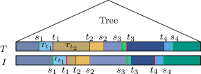
Figure 5: Separators of $I$ and $T$. Here $p=5$. For example, the elements from $I_{t_{1}}$ and $T_{t_{1}}$ lay in intersecting ranges. But the elements from $T_{t_{1}}$ and $T_{t_{2}}$ lay in disjoint ranges. As well as the elements of $I_{t_{1}}$ and $T_{t_{2}}$.

Now consider $x\in S\cup T_{\mathrm{sep}}$. The subsequence $I_{x}$ of $I$ includes all elements $\leq$ $x$ but greater than $y$, the largest element in $S\cup T_{\mathrm{sep}}$ that is less than $x$. Similarly, we define subtree $T_{x}$. We implicitly represent the subsequence $I_{x}$ and subtree $T_{x}$ by $y$ and $x$. Each PE uses binary search to find $y$. For example, PE $i$ calculates the implicit representation of $I_{s_{i}},T_{s_{i}},I_{t_{i}},T_{t_{i}}$. These searches take time at most $\mathcal{O}(\log p)$, since $S$ and $T_{\mathrm{sep}}$ are sorted and we can use binary search. Thus, we split $I$ and $T$ into $2p-1$ parts each: $\mathcal{I}=\{I_{x}:x\in S\cup T_{\mathrm{sep}}\}$ and $\mathcal{T}=\{T_{x}:x\in S\cup T_{\mathrm{sep}}\}$ respectively.

Note that elements of two arbitrary subsequences from $\mathcal{I}\cup\mathcal{T}$ lay in disjoint ranges, except for $I_{x}$ and $T_{x}$ for the same $x\in S\cup T_{\mathrm{sep}}$. Also $|I_{x}|\leq|I|/p$ and $|T_{x}|\leq|T|/p$, since the distances between neighboring separators in $S$ and $T$ are at most $|I|/p$ and $|T|/p$, respectively. See Figure 5.

Split and Insert phases

First, we select $p-1$ separators using uniform selection. Next, we split the tree $T$ into $p$ subtrees $T_{1},\dots,T_{p}$ using the parallel split algorithm from Section III. Finally, we insert the subsequence $I_{i}$ into corresponding subtree $T_{i}$, for $i=1\dots p$, in $\mathcal{O}(|I|/p\log|T|)$ time on a CREW PRAM.

Split and Union phase

Suppose we selected the separators using selection with double binary search. First, we split the sequence $I$ into subsequences $\mathcal{I}$. Next, we split $T$ into subtrees $\mathcal{T}$. For each subtree $T_{x}\in\mathcal{T}$ we split $T$ by the representatives $y$ and $x$ of $T_{x}$ using the parallel split algorithm from Section III.

Now each PE $i$ unions $I_{s_{i}}$ with $T_{s_{i}}$ and $I_{t_{i}}$ with $T_{t_{i}}$ ($s_{i},t_{i}\in S\cup T_{\mathrm{sep}}$) using the sequential union algorithm from Section II. This algorithm unions $I_{x}\in\mathcal{I}$ and $T_{x}$ in $\mathcal{O}(|I_{x}|\log\frac{|T_{x}|}{|I_{x}|})$ time. Hence, the union phase can be done in $\mathcal{O}(|I|/p\log\frac{|T|}{|I|})$ time, because $|I_{x}|\leq|I|/p$ and $|T_{x}|\leq|T|/p$ for any $x\in S\cup T_{\mathrm{sep}}$ and because for $|T_{x}|\geq e|I_{x}|$, $|I_{x}|\log\frac{|T_{x}|}{|I_{x}|}$ is maximized for the largest allowed value of $|I_{x}|$. For the remaining cases, we can use that the log term is bounded by a constant anyway.

Join Phase

We join the trees $T_{1},\dots,T_{k}$ ($k=p$ or $2p-1$) into the tree $T$ in $\mathcal{O}(\log p+\log|T|)$ time on a CREW PRAM using the non-optimal parallel join algorithm from Section IV. We use the non-optimal version, because it maintains subtree sizes in nodes of trees.

VII Operations on Two Trees

Theorem 5.

Let $U$ and $T$ denote search trees ($|U|\leq|T|$) that we identify with sets of elements. Let $k=\max\{|U|,|T|\}$ and $n=\max\{k,p\}$. Search trees for $U\cup T$ (union), $U\cap T$ (intersection), $U\setminus T$ (difference), and $U\bigtriangleup T$ (symmetric difference) can be computed in time $\mathcal{O}(k/p\log\frac{n}{k}+\log n)$.

Union

Computing the union of two trees $U$ and $T$ can be implemented by viewing the smaller tree as a sorted sequence of insertions. Then we can extract the elements of $U$ in sorted order using work $\mathcal{O}(k)$ and span $\mathcal{O}(\log n)$. Adding the complexity of a bulk insertion from Theorem 4 we get total time $\mathcal{O}(k/p\log\frac{n}{k}+\log n)$.

Intersection

We perform a bulk search for the elements of $U$ in $T$ in time $\mathcal{O}(k/p\log\frac{n}{k}+\log n)$ and build a search tree from this sorted sequence in time $\mathcal{O}(k/p+\log n)$.

Set Difference $T\setminus U$

If $|T|\geq|U|$ we can interpret $U$ as a sequence of deletions. This yields parallel time $\mathcal{O}(k/p\log\frac{n}{k}+\log n)$. If $|U|>|T|$, we first intersect $U$ and $T$ in time $\mathcal{O}(k/p\log\frac{n}{k}+\log n)$ and then compute the set difference $T\setminus U=T\setminus(T\cap U)$ in time $\mathcal{O}(k/p\log\frac{n}{k}+\log n)$.

Symmetric Difference

We use the results for union and difference and apply the definition $U\bigtriangleup T=(U\setminus T)\cup(T\setminus U)$.

VIII Experiments

In this section, we evaluate the performance of our parallel $(a,b)$-trees and compare them to the several number of contestants. We also study our basic operations, join and split, in isolation.

Methodology

We implemented our algorithms using C++. Our implementation uses the C++11 multi-threading library (implemented using the POSIX thread library) and an allocator tbb::scalable_allocator from the Intel Threading-Building Blocks (TBB) library. All binaries are built using g++-4.9.2 with the -O3 flag. We run our experiments on Intel Xeon E5-2650v2 (2 sockets, 8 cores with Hyper-Threading, 32 threads) running at 2.6 GHz with 128GB RAM. To decrease scheduling effects, we pin one thread to each core.

Each test can be described by the size of an initial $(4,8)$-tree ($T$), the size of a bulk update ($B$), the number of iterations ($I$) and the number of processors ($p$). Each key is a 32-bit integer. In the beginning of each test we construct an initial tree. During each iteration we perform an incremental bulk update. We use a uniform, skewed uniform, normal and increasing uniform distributions to generate an initial tree and bulk updates in most of the tests. The skewed distribution generates keys in smaller range than a uniform distribution. The increasing uniform distribution generates the keys of a bulk update such that the keys of the current bulk update are greater than the keys of the previous bulk updates.

Split algorithms

We present a comparison of the sequential split algorithm and the parallel split algorithm from Section III. We split an initial tree into $31$ trees using $30$ sorted separators. The sequential algorithm splits the pre-constructed tree into two trees using the first separator and the split operation from Section II. Next, it continues to split using the second separator, and so on. Figure 6 shows the running times of the tests with a uniform distribution (other distributions have almost the same running times). The parallel split algorithm outperforms the sequential algorithm by a factor of $8.1$. Also we run experiments with $p=16$ and split an initial tree into $16$ trees. The speed-up of the parallel split is $4.6$.

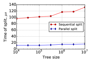
Figure 6: Comparison of split algorithms. $T=\sqrt{10}^{i},i=8,\dots,14$, and $p=31$

Join algorithms

We present a comparison of different join algorithms. We join $31$ trees using the following three algorithms: (1) SJ is a sequential join algorithm. It joins the first tree to the second tree using join operation from Section II. Next, it joins the result of previous join and the third tree, and so on. (2) PPJ is a parallel pairwise join algorithm that joins pairs of trees in parallel from Section IV. (3) PJ is a parallel join algorithm from Section V. Figure 7 shows the running times of the tests with a uniform distribution (other distributions have almost the same running times). The PJ algorithm is worse than the SJ and the PPJ algorithm by a factors of $1.9$ and $3.4$, respectively. The PPJ algorithm has a speed-up of $1.8$ compared to the SJ. This can be explained by the involved synchronization overhead. In the experiments with $p=16$ and $16$ trees the PPJ and SJ algorithms show the same running times. We explain this by the fact that hyper-threading advantages when there are a lot of dereferences of pointers and the number of trees is nearly doubled.

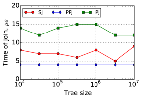
Figure 7: Comparison of join algorithms. $T=\sqrt{10}^{i},i=8,\dots,14$, and $p=31$

Additionally, we measure the number of visited nodes during the course of the join algorithms to show the theoretical advantage of the the PJ algorithm over the the SJ and the PPJ algorithms. Figure 8 shows the results of the tests with two initial trees, which are built using a uniform and a skewed uniform(suffix ”_SU”) distribution.

The PJ algorithm visits significantly less nodes than the SJ algorithm (by a factor of $2.8$) on the tests with a uniform distributions. But it visits almost the same number of nodes as the PPJ algorithm. The PJ_SU algorithm visits less nodes than the SJ_SU and the PPJ_SU algorithms (by factor of $3.9$ and $1.3$, respectively). We explain this by the fact that a skewed uniform distribution constructs an initial tree that is split into $31$ trees, such that the first tree is significantly higher than other trees. Therefore, the algorithms SJ and PPJ visit more nodes than the algorithm PJ during the access to a spine node by rank. This suggests that the PJ algorithm may outperform its competitors on instances with deeper trees and/or additional work per node (for example, an I/O operation per node in external B-tree).

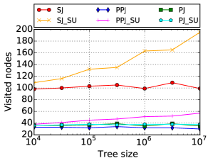
Figure 8: Visited nodes of the join algorithms. $T=\sqrt{10}^{i},i=8,\dots,14$, and $p=31$

Comparison of parallel search trees

Here we compare our sequential and parallel implementations of search trees and four competitors:

1. Seq is a $(4,8)$-tree with a sequential bulk updates from Section II;

2. PS_PPJ is a $(4,8)$-tree with a parallel split phase, a union phase and a parallel pairwise join phase;

3. PWBT is a Parallel Weight-Balanced B-tree [8];

4. PRBT is a Parallel Red-Black Tree [9];

5. PBST is a Parallel Binary Search Tree [1] (we compile it using g++-4.8 compiler with Cilk support).

Figure 9 shows the measurements of the tests with a uniform distribution, where $T=100M,B=16,\sqrt{10}^{i},i=4,\dots,14$ ($I=10000$ for $B=16,\dots,100K$ and $I=4G/B$ for $B=316227,\dots,10M$) and $p=16$ (we use 16 cores, since the insert phase is cache-efficient and hyper-threading does not improve performance). We achieve relative speedup up to 12 over sequential $(a,b)$-trees. Even for very small batches of size 100 we observe some speedup. Note that the speed-ups of the join and split phases are less than 12. But they do not affect the total speed-up, since the time of the insertion phase dominates them.

On average, our algorithms are $1.8$ times faster than a PWBT. We outperform the PWBT since a subtree rebalancing (linear of the subtree size) can occur during an insert operation. Also our data structure is $5.5$ times faster than a PRBT, $5.7$ times faster than a PBST and $10.7$ faster than a Seq. Note that the PRBT and the PBST failed in the last four tests due to the lack of memory space. Hence, we expect even greater speed-up of our algorithms compare to them. For small batches, the speedup is larger which we attribute to the startup overhead of using Cilk.

Additionally, we run the tests for the PS_PPJ and the fastest competitor the PWBT with the same parameters using a normal, skewed uniform and increasing uniform distributions to generate bulk updates. They perform faster in these tests than in the tests with a uniform distribution due to the improved cache locality. Although a subtree rebalancings in PWBT last longer than in the tests with a uniform distributions, they occur less frequently. On average, the PS_PPJ is $2.0$, $2.6$ and $2.1$ times faster than the PWBT in tests with a normal, skewed uniform and increasing uniform distributions respectively.

Figure 10 shows another comparison of the PS_PPJ with the PWBT. This plot shows the worst-case guaranties of the PS_PPJ. The spikes on the plot of the PWBT are due to the amortized cost of operations. We conclude that the PS_PPJ is preferable in real-time applications where latency is crucial.

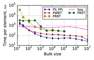
Figure 9: Bulk updates algorithms.

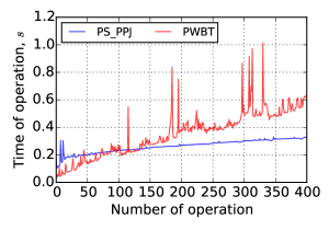
Figure 10: Running time of all operations. $T=100M,B=10M$ and $I=400$

References

- [1] Guy E. Blelloch, Daniel Ferizovic, and Yihan Sun, Parallel ordered sets using join, CoRR abs/1602.02120 (2016).
- [2] Guy E. Blelloch and Margaret Reid-Miller, Fast set operations using treaps, 10th ACM Symposium on Parallel Algorithms and Architectures, SPAA, 1998, pp. 16–26.
- [3] Gerth S. Brodal, Christos Makris, and Kostas Tsichlas, Purely functional worst case constant time catenable sorted lists, ESA, LNCS, vol. 4168, Springer, 2006, pp. 172–183.
- [4] Nathan G. Bronson, Jared Casper, Hassan Chafi, and Kunle Olukotun, A practical concurrent binary search tree, 15th Symposium on Principles and Practice of Parallel Programming (PPoPP), ACM, 2010, pp. 257–268.
- [5] Mark R. Brown and Robert E. Tarjan, A fast merging algorithm, J. ACM 26 (1979), no. 2, 211–226.
- [6] Mark R. Brown and Robert E. Tarjan, Design and analysis of a data structure for representing sorted lists, SIAM J. Comput. 9 (1980), no. 3, 594–614.
- [7] Thomas H. Cormen, Charles E. Leiserson, Ronald L. Rivest, and Clifford Stein, Introduction to algorithms, third edition, 3rd ed., The MIT Press, 2009.
- [8] Stephan Erb, Moritz Kobitzsch, and Peter Sanders, Parallel bi-objective shortest paths using weight-balanced B-trees with bulk updates, 13th Symposium on Experimental Algorithms (SEA), LNCS, vol. 8504, Springer, 2014, pp. 111–122.
- [9] Leonor Frias and Johannes Singler, Parallelization of bulk operations for STL dictionaries, Euro-Par Workshops, LNCS, vol. 4854, Springer, 2007, pp. 49–58.
- [10] Maurice Herlihy, Yossi Lev, Victor Luchangco, and Nir Shavit, A provably correct scalable skiplist, 10th International Conference On Principles Of Distributed Systems (OPODIS), 2006.
- [11] Lisa Higham and Eric Schenk, Maintaining B-trees on an EREW PRAM, Journal of Parallel and Distributed Computing 22 (1994), no. 2, 329–335.
- [12] Scott Huddleston and Kurt Mehlhorn, A new data structure for representing sorted lists, Acta Inf. 17 (1982), 157–184.
- [13] Joseph F. JaJa, An introduction to parallel algorithms, Addison Wesley Longman Publishing Co., Inc., Redwood City, CA, USA, 1992.
- [14] Haim Kaplan and Robert E. Tarjan, Purely functional representations of catenable sorted lists., 28th ACM Symp. on Theory of Computing (STOC), 1996, pp. 202–211.
- [15] Jyrki Katajainen, Efficient parallel algorithms for manipulating sorted sets, 17th Annual Computer Science Conf., U. of Canterbury, 1994, pp. 281–288.
- [16] Philip L Lehman and Bing Yao, Efficient locking for concurrent operations on B-trees, ACM Transactions on Database Systems (TODS) 6 (1981), no. 4, 650–670.
- [17] Kurt Mehlhorn and Peter Sanders, Algorithms and data structures: The basic toolbox, Springer, 2008.
- [18] Alistair Moffat, Ola Petersson, and Nicholas C. Wormald, Sorting and/by merging finger trees, Algorithms and Computation, LNCS, vol. 650, Springer, 1992, pp. 499–508.
- [19] Heejin Park and Kunsoo Park, Parallel algorithms for red-black trees, Theoretical Computer Science 262 (2001), 415 – 435.
- [20] Wolfgang Paul, Uzi Vishkin, and Hubert Wagener, Parallel dictionaries on 2–3 trees, 10th Interntaional Colloquium on Automata, Languages and Programming (ICALP), vol. 154, Springer, 1983, pp. 597–609.
- [21] Jason Sewall et al., PALM: Parallel architecture-friendly latch-free modifications to B+ trees on many-core processors, PVLDB 4 (2011), no. 11, 795–806.
- [22] Yossi Shiloach and Uzi Vishkin, Finding the maximum, merging, and sorting in a parallel computation model., J. Algorithms 2 (1981), 88–102.