On the strong coupling $N^{(*)}N^{(*)}\pi$

We study the strong vertices $N^{*}N\pi$, $N^{*}N^{*}\pi$ and $NN\pi$ in QCD, where $N^{*}$ denotes the negative parity $N(1535)$ state. We use the most general form of the interpolating currents to calculate the corresponding strong coupling constants. It is obtained that the coupling associated to $N^{*}N\pi$ vertex is strongly suppressed compared to those related to two other vertices. The strong coupling corresponding to $N^{*}N^{*}\pi$ is obtained to be roughly half of that of $NN\pi$ vertex. We compare the obtained results on $N^{*}N\pi$ and $NN\pi$ vertices with the existing predictions of other theoretical studies as well as those extracted from the experimental data.

PACS number(s):14.20.Dh, 14.40.Be, 13.75.Gx, 11.55.Hx

1 Introduction

In hadron physics the strong couplings among various particles play essential roles in understanding of the strong interaction and the nature and structure of the participating particles. Hence, one needs the precise determination of these strong coupling constants. Especially, due to the limited experimental information related to the decay properties of the negative parity baryons, the theoretical studies in this area can provide effective contributions. Beside the properties of negative parity baryons, reinvestigation of the coupling form factor of the pion-nucleon and comparisons of the results with the known theoretical and empirical results may supply a better understanding about the nonperturbative nature of QCD.

The properties of negative parity nucleon, such as mass and the other spectroscopic properties, were studied extensively (see for instance the Ref. [1, 2, 3, 4, 5] and the references therein). Beside the spectral properties, its magnetic moment was analyzed using QCD sum rules [6] and effective Hamiltonian [7] approaches. The light cone QCD sum rule was applied to obtain the electromagnetic transition form factors of $\gamma^{*}N\rightarrow N(1535)$ and $\gamma^{\ast}N\rightarrow N^{\ast}(1520)$  [8, 9]. The radiative transition of negative to positive parity nucleon was also studied in Ref. [10]. This work is devoted to the study of the strong coupling constants among the negative parity $N^{*}(1535)$, nucleon and pion in QCD. Such type of investigations were done extensively using either three point QCD sum rules with Ioffe current or light cone QCD sum rules and some other methods. One can find some of them in Refs. [11, 12, 13, 14, 15, 16, 17, 18, 19, 20, 21, 22, 23, 24, 25, 26, 27, 28] and the references therein. In the present study, regarding the mass difference between the initial and final nucleons in the considered transitions, the three point QCD sum rule method is applied. This method [29] is one of the most powerful method among nonperturbative approaches and was used extensively and successfully to obtain the hadronic properties. We consider the three-point correlation function with the most general form of the interpolating currents for the positive and negative parity nucleons.

The outline of the article is as follows. In section 2 the details of the QCD sum rules calculation for the considered transitions are presented. Section 3 is devoted to the numerical results and conclusion.

2 The strong coupling form factors between the positive and negative parity nucleons and pion

This section presents some details of the calculations of the strong coupling form factors between the positive and negative parity nucleons and pion using the QCD sum rule method. The starting point is to consider the following correlation function in terms of the interpolating fields of the considered states:

$$\Pi(q)=i^{2}\int d^{4}x~{}\int d^{4}y~{}e^{-ip\cdot x}~{}e^{ip^{\prime}\cdot y}~{}{\langle}0|{\cal T}\left(J_{N^{(^{\prime}*)}}(y)~{}J_{\pi}(0)~{}\bar{J}_{N^{(^{\prime}*)}}(x)\right)|0{\rangle},$$ (1)

where ${\cal T}$ is the time ordering operator and $q=p-p^{\prime}$ is the transferred momentum. In this equation $J_{i}$ represent the interpolating fields of nucleon and $\pi$ meson. $N$ and $N^{*}$ denote the positive parity ground state and the negative parity $N(1535)$, respectively. Here, $N^{\prime}$ stands for the excited positive parity state $N(1440)$, that also couples to the nucleon currents and we shall take into account its contribution to the correlation function. We calculate this correlation function in terms of physical and OPE (operator product expansion) sides. By matching these two representations, the corresponding strong coupling form factors are found. To suppress the contributions of the higher states and continuum, a double Borel transformation with respect to $p^{2}$ and $p^{\prime 2}$ together with continuum subtractions are applied to both sides.

2.1 Physical Side

For the calculation of the physical side complete sets of appropriate $N$, $N^{*}$, $N^{{}^{\prime}}$ and $\pi$ hadronic states carrying the same quantum numbers with the corresponding interpolating currents are placed into the correlation function. Integrations over $x$ and $y$ gives

$$\Pi^{Phy}(q) = \frac{\langle 0\mid J_{N}\mid N(p^{\prime},s^{\prime})\rangle\langle 0\mid J_{\pi}\mid\pi(q)\rangle\langle N(p^{\prime},s^{\prime})\pi(q)\mid N(p,s)\rangle\langle N(p,s)\mid\bar{J}_{N}\mid 0\rangle}{(p^{2}-m_{N}^{2})(p^{\prime^{2}}-m_{N}^{2})(q^{2}-m_{\pi}^{2})}$$ (2)

$$+ \frac{\langle 0\mid J_{N^{*}}\mid N^{*}(p^{\prime},s^{\prime})\rangle\langle 0\mid J_{\pi}\mid\pi(q)\rangle\langle N^{*}(p^{\prime},s^{\prime})\pi(q)\mid N^{*}(p,s)\rangle\langle N^{*}(p,s)\mid\bar{J}_{N^{*}}\mid 0\rangle}{(p^{2}-m_{N^{*}}^{2})(p^{\prime^{2}}-m_{N^{*}}^{2})(q^{2}-m_{\pi}^{2})}$$

$$+ \frac{\langle 0\mid J_{N}\mid N(p^{\prime},s^{\prime})\rangle\langle 0\mid J_{\pi}\mid\pi(q)\rangle\langle N(p^{\prime},s^{\prime})\pi(q)\mid N^{*}(p,s)\rangle\langle N^{*}(p,s)\mid\bar{J}_{N^{*}}\mid 0\rangle}{(p^{2}-m_{N^{*}}^{2})(p^{\prime^{2}}-m_{N}^{2})(q^{2}-m_{\pi}^{2})}$$

$$+ \frac{\langle 0\mid J_{N^{*}}\mid N^{*}(p^{\prime},s^{\prime})\rangle\langle 0\mid J_{\pi}\mid\pi(q)\rangle\langle N^{*}(p^{\prime},s^{\prime})\pi(q)\mid N(p,s)\rangle\langle N(p,s)\mid\bar{J}_{N}\mid 0\rangle}{(p^{2}-m_{N}^{2})(p^{\prime^{2}}-m_{N^{*}}^{2})(q^{2}-m_{\pi}^{2})}$$

$$+ \frac{\langle 0\mid J_{N^{\prime}}\mid N^{\prime}(p^{\prime},s^{\prime})\rangle\langle 0\mid J_{\pi}\mid\pi(q)\rangle\langle N^{\prime}(p^{\prime},s^{\prime})\pi(q)\mid N^{\prime}(p,s)\rangle\langle N^{\prime}(p,s)\mid\bar{J}_{N^{\prime}}\mid 0\rangle}{(p^{2}-m_{N^{\prime}}^{2})(p^{\prime^{2}}-m_{N^{\prime}}^{2})(q^{2}-m_{\pi}^{2})}$$

$$+ \frac{\langle 0\mid J_{N}\mid N(p^{\prime},s^{\prime})\rangle\langle 0\mid J_{\pi}\mid\pi(q)\rangle\langle N(p^{\prime},s^{\prime})\pi(q)\mid N^{\prime}(p,s)\rangle\langle N^{\prime}(p,s)\mid\bar{J}_{N^{\prime}}\mid 0\rangle}{(p^{2}-m_{N^{\prime}}^{2})(p^{\prime^{2}}-m_{N}^{2})(q^{2}-m_{\pi}^{2})}$$

$$+ \frac{\langle 0\mid J_{N^{\prime}}\mid N^{\prime}(p^{\prime},s^{\prime})\rangle\langle 0\mid J_{\pi}\mid\pi(q)\rangle\langle N^{\prime}(p^{\prime},s^{\prime})\pi(q)\mid N(p,s)\rangle\langle N(p,s)\mid\bar{J}_{N}\mid 0\rangle}{(p^{2}-m_{N}^{2})(p^{\prime^{2}}-m_{N^{\prime}}^{2})(q^{2}-m_{\pi}^{2})}$$

$$+ \frac{\langle 0\mid J_{N^{*}}\mid N^{*}(p^{\prime},s^{\prime})\rangle\langle 0\mid J_{\pi}\mid\pi(q)\rangle\langle N^{*}(p^{\prime},s^{\prime})\pi(q)\mid N^{\prime}(p,s)\rangle\langle N^{\prime}(p,s)\mid\bar{J}_{N^{\prime}}\mid 0\rangle}{(p^{2}-m_{N^{\prime}}^{2})(p^{\prime^{2}}-m_{N^{*}}^{2})(q^{2}-m_{\pi}^{2})}$$

$$+ \frac{\langle 0\mid J_{N^{\prime}}\mid N^{\prime}(p^{\prime},s^{\prime})\rangle\langle 0\mid J_{\pi}\mid\pi(q)\rangle\langle N^{\prime}(p^{\prime},s^{\prime})\pi(q)\mid N^{*}(p,s)\rangle\langle N^{*}(p,s)\mid\bar{J}_{N^{*}}\mid 0\rangle}{(p^{2}-m_{N^{*}}^{2})(p^{\prime^{2}}-m_{N^{\prime}}^{2})(q^{2}-m_{\pi}^{2})}$$

$$+ \cdots~{}.$$

where we included contributions of both positive and negative parity nucleons and the contributions coming from the higher states and continuum are represented by $\cdots$. The matrix elements emerging in this result are parameterized in terms of the residues $\lambda_{N}$, $\lambda_{N^{*}}$ and $\lambda_{N^{{}^{\prime}}}$, the spinors $u_{N}$, $u_{N^{*}}$ and $u_{N^{{}^{\prime}}}$ , the leptonic decay constant of $\pi$ meson as well as the strong couplings $g_{NN\pi}$, $g_{N^{*}N^{*}\pi}$, $g_{N^{{}^{\prime}}N^{{}^{\prime}}\pi}$, $g_{NN^{*}\pi}$, $g_{N^{*}N\pi}$, $g_{NN^{{}^{\prime}}\pi}$, $g_{N^{{}^{\prime}}N\pi}$, $g_{N^{{}^{\prime}}N^{*}\pi}$ and $g_{N^{*}N^{{}^{\prime}}\pi}$ as

$$\langle 0\mid J_{N^{(\prime)}}\mid N^{(\prime)}(p^{\prime},s^{\prime})\rangle = \lambda_{N^{(^{\prime})}}u_{N^{(\prime)}}(p^{\prime},s^{\prime}),$$

$$\langle 0\mid J_{N^{*}}\mid N^{*}(p^{\prime},s^{\prime})\rangle = \lambda_{N^{*}}\gamma_{5}u_{N^{*}}(p^{\prime},s^{\prime}),$$

$$\langle 0\mid J_{\pi}\mid\pi(q)\rangle = i\frac{f_{\pi}m_{\pi}^{2}}{m_{u}+m_{d}},$$

$$\langle N^{(\prime)}(p^{\prime},s^{\prime})\pi(q)\mid N^{(\prime)}(p,s)\rangle = g_{N^{(\prime)}N^{(\prime)}\pi}\bar{u}_{N^{(\prime)}}(p^{\prime},s^{\prime})i\gamma_{5}u_{N^{(\prime)}}(p,s),$$

$$\langle N^{*}(p^{\prime},s^{\prime})\pi(q)\mid N^{*}(p,s)\rangle = g_{N^{*}N^{*}\pi}\bar{u}_{N^{*}}(p^{\prime},s^{\prime})i\gamma_{5}u_{N^{*}}(p,s),$$

$$\langle N^{*}(p^{\prime},s^{\prime})\pi(q)\mid N^{(\prime)}(p,s)\rangle = g_{N^{(\prime)}N^{*}\pi}\bar{u}_{N^{*}}(p^{\prime},s^{\prime})iu_{N^{(\prime)}}(p,s),$$

$$\langle N^{(\prime)}(p^{\prime},s^{\prime})\pi(q)\mid N^{*}(p,s)\rangle = g_{N^{*}N^{(\prime)}\pi}\bar{u}_{N^{(\prime)}}(p^{\prime},s^{\prime})iu_{N^{*}}(p,s).$$ (3)

Using these parametrizations and summation over Dirac spinors via

$$\sum_{s}u_{N}(p,s)\bar{u}_{N}(p,s)=\not\!p+m_{N}$$ (4)

in Eq.(2), we get

$$\Pi^{Phy}(q) = i^{2}\frac{f_{\pi}m_{\pi}^{2}}{m_{u}+m_{d}}\Bigg{\{}g_{NN\pi}\lambda_{N}^{2}\frac{(\not\!p^{\prime}+m_{N})\gamma_{5}(\not\!p+m_{N})}{(p^{2}-m_{N}^{2})(p^{\prime^{2}}-m_{N}^{2})(q^{2}-m_{\pi}^{2})}$$ (5)

$$- g_{N^{*}N^{*}\pi}\lambda_{N^{*}}^{2}\frac{(\not\!p^{\prime}-m_{N^{*}})\gamma_{5}(\not\!p-m_{N^{*}})}{(p^{2}-m_{N^{*}}^{2})(p^{\prime^{2}}-m_{N^{*}}^{2})(q^{2}-m_{\pi}^{2})}$$

$$+ g_{N^{*}N\pi}\lambda_{N}\lambda_{N^{*}}\frac{(\not\!p^{\prime}+m_{N})\gamma_{5}(\not\!p-m_{N^{*}})}{(p^{2}-m_{N^{*}}^{2})(p^{\prime^{2}}-m_{N}^{2})(q^{2}-m_{\pi}^{2})}$$

$$- g_{NN^{*}\pi}\lambda_{N}\lambda_{N^{*}}\frac{(\not\!p^{\prime}-m_{N^{*}})\gamma_{5}(\not\!p+m_{N})}{(p^{2}-m_{N}^{2})(p^{\prime^{2}}-m_{N^{*}}^{2})(q^{2}-m_{\pi}^{2})}$$

$$+ g_{N^{\prime}N^{\prime}\pi}\lambda_{N^{\prime}}^{2}\frac{(\not\!p^{\prime}+m_{N^{\prime}})\gamma_{5}(\not\!p+m_{N^{\prime}})}{(p^{2}-m_{N^{\prime}}^{2})(p^{\prime^{2}}-m_{N^{\prime}}^{2})(q^{2}-m_{\pi}^{2})}$$

$$+ g_{N^{\prime}N\pi}\lambda_{N}\lambda_{N^{\prime}}\frac{(\not\!p^{\prime}+m_{N})\gamma_{5}(\not\!p+m_{N^{\prime}})}{(p^{2}-m_{N^{\prime}}^{2})(p^{\prime^{2}}-m_{N}^{2})(q^{2}-m_{\pi}^{2})}$$

$$+ g_{NN^{\prime}\pi}\lambda_{N}\lambda_{N^{\prime}}\frac{(\not\!p^{\prime}+m_{N^{\prime}})\gamma_{5}(\not\!p+m_{N})}{(p^{2}-m_{N}^{2})(p^{\prime^{2}}-m_{N^{\prime}}^{2})(q^{2}-m_{\pi}^{2})}$$

$$- g_{N^{\prime}N^{*}\pi}\lambda_{N^{\prime}}\lambda_{N^{*}}\frac{(\not\!p^{\prime}-m_{N^{*}})\gamma_{5}(\not\!p+m_{N^{\prime}})}{(p^{2}-m_{N^{\prime}}^{2})(p^{\prime^{2}}-m_{N^{*}}^{2})(q^{2}-m_{\pi}^{2})}$$

$$+ g_{N^{*}N^{\prime}\pi}\lambda_{N^{\prime}}\lambda_{N^{*}}\frac{(\not\!p^{\prime}+m_{N^{\prime}})\gamma_{5}(\not\!p-m_{N^{*}})}{(p^{2}-m_{N^{*}}^{2})(p^{\prime^{2}}-m_{N^{\prime}}^{2})(q^{2}-m_{\pi}^{2})}\Bigg{\}}.$$

After application of a double Borel transformation with respect to the initial and final momenta the final result for the physical side in terms of different Dirac structures becomes

$$\widehat{\textbf{B}}\Pi^{Phys}(q) = i^{2}\frac{f_{\pi}m_{\pi}^{2}}{(m_{u}+m_{d})(q^{2}-m_{\pi}^{2})}\Big{(}\Phi_{1}\not\!p\not\!q\gamma_{5}+\Phi_{2}\not\!p\gamma_{5}+\Phi_{3}\not\!q\gamma_{5}+\Phi_{4}\gamma_{5}\Big{)},$$ (6)

where

$$\Phi_{1} = -g_{NN\pi}\lambda_{N}^{2}e^{-\frac{m_{N}^{2}}{M^{2}}-\frac{m_{N}^{2}}{M^{\prime^{2}}}}+g_{NN^{*}\pi}\lambda_{N}\lambda_{N^{*}}e^{-\frac{m_{N}^{2}}{M^{2}}-\frac{m_{N^{*}}^{2}}{M^{\prime^{2}}}}-g_{N^{*}N\pi}\lambda_{N}\lambda_{N^{*}}e^{-\frac{m_{N^{*}}^{2}}{M^{2}}-\frac{m_{N}^{2}}{M^{\prime^{2}}}}$$

$$+ g_{N^{*}N^{*}\pi}\lambda_{N^{*}}^{2}e^{-\frac{m_{N^{*}}^{2}}{M^{2}}-\frac{m_{N^{*}}^{2}}{M^{\prime^{2}}}}-g_{NN^{\prime}\pi}\lambda_{N}\lambda_{N^{\prime}}e^{-\frac{m_{N}^{2}}{M^{2}}-\frac{m_{N^{\prime}}^{2}}{M^{\prime^{2}}}}-g_{N^{\prime}N\pi}\lambda_{N}\lambda_{N^{\prime}}e^{-\frac{m_{N^{\prime}}^{2}}{M^{2}}-\frac{m_{N}^{2}}{M^{\prime^{2}}}}$$

$$- g_{N^{\prime}N^{\prime}\pi}\lambda_{N^{\prime}}^{2}e^{-\frac{m_{N^{\prime}}^{2}}{M^{2}}-\frac{m_{N^{\prime}}^{2}}{M^{\prime^{2}}}}+g_{N^{\prime}N^{*}\pi}\lambda_{N^{\prime}}\lambda_{N^{*}}e^{-\frac{m_{N^{\prime}}^{2}}{M^{2}}-\frac{m_{N^{*}}^{2}}{M^{\prime^{2}}}}-g_{N^{*}N^{\prime}\pi}\lambda_{N^{\prime}}\lambda_{N^{*}}e^{-\frac{m_{N^{*}}^{2}}{M^{2}}-\frac{m_{N^{\prime}}^{2}}{M^{\prime^{2}}}},$$

$$\Phi_{2} = -g_{NN^{*}\pi}\lambda_{N}\lambda_{N^{*}}(m_{N}+m_{N^{*}})e^{-\frac{m_{N}^{2}}{M^{2}}-\frac{m_{N^{*}}^{2}}{M^{\prime^{2}}}}-g_{N^{*}N\pi}\lambda_{N}\lambda_{N^{*}}(m_{N}+m_{N^{*}})e^{-\frac{m_{N^{*}}^{2}}{M^{2}}-\frac{m_{N}^{2}}{M^{\prime^{2}}}}$$

$$- g_{NN^{\prime}\pi}\lambda_{N}\lambda_{N^{\prime}}(m_{N^{\prime}}-m_{N})e^{-\frac{m_{N}^{2}}{M^{2}}-\frac{m_{N^{\prime}}^{2}}{M^{\prime^{2}}}}+g_{N^{\prime}N\pi}\lambda_{N}\lambda_{N^{\prime}}(m_{N^{\prime}}-m_{N})e^{-\frac{m_{N^{\prime}}^{2}}{M^{2}}-\frac{m_{N}^{2}}{M^{\prime^{2}}}}$$

$$- g_{N^{\prime}N^{*}\pi}\lambda_{N^{\prime}}\lambda_{N^{*}}(m_{N^{\prime}}+m_{N^{*}})e^{-\frac{m_{N^{\prime}}^{2}}{M^{2}}-\frac{m_{N^{*}}^{2}}{M^{\prime^{2}}}}-g_{N^{*}N^{\prime}\pi}\lambda_{N^{\prime}}\lambda_{N^{*}}(m_{N^{\prime}}+m_{N^{*}})e^{-\frac{m_{N^{*}}^{2}}{M^{2}}-\frac{m_{N^{\prime}}^{2}}{M^{\prime^{2}}}},$$

$$\Phi_{3} = -g_{NN\pi}\lambda_{N}^{2}m_{N}e^{-\frac{m_{N}^{2}}{M^{2}}-\frac{m_{N}^{2}}{M^{\prime^{2}}}}+g_{NN^{*}\pi}\lambda_{N}\lambda_{N^{*}}m_{N}e^{-\frac{m_{N}^{2}}{M^{2}}-\frac{m_{N^{*}}^{2}}{M^{\prime^{2}}}}+g_{N^{*}N\pi}\lambda_{N}\lambda_{N^{*}}m_{N^{*}}e^{-\frac{m_{N^{*}}^{2}}{M^{2}}-\frac{m_{N}^{2}}{M^{\prime^{2}}}}$$

$$- g_{N^{*}N^{*}\pi}\lambda_{N^{*}}^{2}m_{N^{*}}e^{-\frac{m_{N^{*}}^{2}}{M^{2}}-\frac{m_{N^{*}}^{2}}{M^{\prime^{2}}}}-g_{NN^{\prime}\pi}\lambda_{N}\lambda_{N^{\prime}}m_{N}e^{-\frac{m_{N}^{2}}{M^{2}}-\frac{m_{N^{\prime}}^{2}}{M^{\prime^{2}}}}-g_{N^{\prime}N\pi}\lambda_{N}\lambda_{N^{\prime}}m_{N^{\prime}}e^{-\frac{m_{N^{\prime}}^{2}}{M^{2}}-\frac{m_{N}^{2}}{M^{\prime^{2}}}}$$

$$- g_{N^{\prime}N^{\prime}\pi}\lambda_{N^{\prime}}^{2}m_{N^{\prime}}e^{-\frac{m_{N^{\prime}}^{2}}{M^{2}}-\frac{m_{N^{\prime}}^{2}}{M^{\prime^{2}}}}+g_{N^{\prime}N^{*}\pi}\lambda_{N^{\prime}}\lambda_{N^{*}}m_{N^{\prime}}e^{-\frac{m_{N^{\prime}}^{2}}{M^{2}}-\frac{m_{N^{*}}^{2}}{M^{\prime^{2}}}}+g_{N^{*}N^{\prime}\pi}\lambda_{N^{\prime}}\lambda_{N^{*}}m_{N^{*}}e^{-\frac{m_{N^{*}}^{2}}{M^{2}}-\frac{m_{N^{\prime}}^{2}}{M^{\prime^{2}}}},$$

$$\Phi_{4} = g_{NN\pi}\lambda_{N}^{2}q^{2}e^{-\frac{m_{N}^{2}}{M^{2}}-\frac{m_{N}^{2}}{M^{\prime^{2}}}}-g_{N^{*}N\pi}\lambda_{N}\lambda_{N^{*}}(m_{N}^{2}+m_{N}m_{N^{*}}-q^{2})e^{-\frac{m_{N^{*}}^{2}}{M^{2}}-\frac{m_{N}^{2}}{M^{\prime^{2}}}}$$ (7)

$$- g_{N^{*}N^{*}\pi}\lambda_{N^{*}}^{2}q^{2}e^{-\frac{m_{N^{*}}^{2}}{M^{2}}-\frac{m_{N^{*}}^{2}}{M^{\prime^{2}}}}+g_{NN^{*}\pi}\lambda_{N}\lambda_{N^{*}}(m_{N^{*}}^{2}+m_{N}m_{N^{*}}-q^{2})e^{-\frac{m_{N}^{2}}{M^{2}}-\frac{m_{N^{*}}^{2}}{M^{\prime^{2}}}}$$

$$+ g_{N^{\prime}N\pi}\lambda_{N}\lambda_{N^{\prime}}(-m_{N}^{2}+m_{N}m_{N^{\prime}}+q^{2})e^{-\frac{m_{N^{\prime}}^{2}}{M^{2}}-\frac{m_{N}^{2}}{M^{\prime^{2}}}}+g_{N^{\prime}N^{\prime}\pi}\lambda_{N^{\prime}}^{2}q^{2}e^{-\frac{m_{N^{{}^{\prime}}}^{2}}{M^{2}}-\frac{m_{N^{\prime}}^{2}}{M^{\prime^{2}}}}$$

$$+ g_{NN^{\prime}\pi}\lambda_{N}\lambda_{N^{\prime}}(-m_{N^{\prime}}^{2}+m_{N}m_{N^{\prime}}+q^{2})e^{-\frac{m_{N}^{2}}{M^{2}}-\frac{m_{N^{\prime}}^{2}}{M^{\prime^{2}}}}-g_{N^{*}N^{\prime}\pi}\lambda_{N^{\prime}}\lambda_{N^{*}}(m_{N^{\prime}}^{2}+m_{N^{\prime}}m_{N^{*}}-q^{2})$$

$$\times e^{-\frac{m_{N^{*}}^{2}}{M^{2}}-\frac{m_{N^{\prime}}^{2}}{M^{\prime^{2}}}}+g_{N^{\prime}N^{*}\pi}\lambda_{N^{\prime}}\lambda_{N^{*}}(m_{N^{*}}^{2}+m_{N^{\prime}}m_{N^{*}}-q^{2})e^{-\frac{m_{N^{\prime}}^{2}}{M^{2}}-\frac{m_{N^{*}}^{2}}{M^{\prime^{2}}}}.$$

The $M^{2}$ and $M^{\prime^{2}}$ arising in these results are the Borel mass parameters in the initial and final channels, respectively.

2.2 OPE Side

The OPE side of the correlation function is calculated in deep Euclidean region. To this aim we use the interpolating current

$$J_{N^{(^{\prime}*)}}(y)=2\varepsilon_{ij\ell}\Big{\{}\Big{(}u^{i^{T}}(y)Cd^{j}(y)\Big{)}\gamma_{5}u^{\ell}(y)+\beta\Big{(}u^{i^{T}}(y)C\gamma_{5}d^{j}(y)\Big{)}u^{\ell}(y)\Big{\}},$$ (8)

which couples to the nucleon with both parities as well as

$$J_{\pi}(0)=\frac{1}{\sqrt{2}}\Big{(}\bar{u}(0)i\gamma_{5}u(0)-\bar{d}(0)i\gamma_{5}d(0)\Big{)}.$$ (9)

for the pion. In Eq.(8), $\beta$ is a general mixing parameter (with $\beta=-1$ corresponding to the Ioffe current) that we shall fix it by some physical considerations and $C$ is the charge conjugation operator. The substitution of these interpolating currents in Eq. (1) is followed by possible contractions of all quark pairs via Wick’s theorem, and this leads to

$$\Pi^{OPE}(q) = 2i^{3}\int d^{4}x\int d^{4}ye^{-ip\cdot x}e^{ip^{\prime}\cdot y}\epsilon_{abc}\epsilon_{ij\ell}$$ (10)

$$\times \Bigg{\{}-Tr\Big{[}S_{d}^{bj}(y-x)S_{u}^{\prime^{di}}(-x)\gamma_{5}S_{u}^{\prime^{ad}}(y)\Big{]}\Big{(}\gamma_{5}S_{u}^{c\ell}(y-x)\gamma_{5}\Big{)}$$

$$+ Tr\Big{[}S_{u}^{\prime^{ai}}(y-x)S_{d}^{bj}(y-x)\Big{]}\Big{(}\gamma_{5}S_{u}^{cd}(y)\gamma_{5}S_{u}^{d\ell}(-x)\gamma_{5}\Big{)}$$

$$- \gamma_{5}S_{u}^{ci}(y-x)S_{d}^{\prime^{bj}}(y-x)S_{u}^{ad}(y)\gamma_{5}S_{u}^{d\ell}(-x)\gamma_{5}$$

$$- \gamma_{5}S_{u}^{cd}(y)\gamma_{5}S_{u}^{di}(-x)S_{d}^{\prime^{bj}}(y-x)S_{u}^{a\ell}(y-x)\gamma_{5}$$

$$- Tr\Big{[}S_{u}^{\prime^{ai}}(y-x)S_{d}^{bd}(y)\gamma_{5}S_{d}^{dj}(-x)\Big{]}\Big{(}\gamma_{5}S_{u}^{c\ell}(y-x)\gamma_{5}\Big{)}$$

$$- \gamma_{5}S_{u}^{ci}(y-x)S_{d}^{\prime^{dj}}(-x)\gamma_{5}S_{d}^{\prime^{bd}}(y)S_{u}^{a\ell}(y-x)\gamma_{5}$$

$$- \beta\Bigg{[}Tr\Big{[}S_{d}^{bj}(y-x)\gamma_{5}S_{u}^{\prime^{di}}(-x)\gamma_{5}S_{u}^{\prime^{ad}}(y)\Big{]}\Big{(}\gamma_{5}S_{u}^{c\ell}(y-x)\Big{)}$$

$$+ Tr\Big{[}\gamma_{5}S_{d}^{bj}(y-x)S_{u}^{\prime^{di}}(-x)\gamma_{5}S_{u}^{\prime^{ad}}(y)\Big{]}\Big{(}S_{u}^{c\ell}(y-x)\gamma_{5}\Big{)}$$

$$- Tr\Big{[}\gamma_{5}S_{u}^{\prime^{ai}}(y-x)S_{d}^{bj}(y-x)\Big{]}\Big{(}\gamma_{5}S_{u}^{cd}(y)\gamma_{5}S_{u}^{d\ell}(-x)\Big{)}$$

$$- Tr\Big{[}S_{u}^{\prime^{ai}}(y-x)\gamma_{5}S_{d}^{bj}(y-x)\Big{]}\Big{(}S_{u}^{cd}(y)\gamma_{5}S_{u}^{d\ell}(-x)\gamma_{5}\Big{)}$$

$$+ \gamma_{5}S_{u}^{ci}(y-x)\gamma_{5}S_{d}^{\prime^{bj}}(y-x)S_{u}^{ad}(y)\gamma_{5}S_{u}^{d\ell}(-x)$$

$$+ S_{u}^{ci}(y-x)S_{d}^{\prime^{bj}}(y-x)\gamma_{5}S_{u}^{ad}(y)\gamma_{5}S_{u}^{d\ell}(-x)\gamma_{5}$$

$$+ S_{u}^{cd}(y)\gamma_{5}S_{u}^{di}(-x)S_{d}^{\prime^{bj}}(y-x)\gamma_{5}S_{u}^{a\ell}(y-x)\gamma_{5}$$

$$+ \gamma_{5}S_{u}^{cd}(y)\gamma_{5}S_{u}^{di}(-x)\gamma_{5}S_{d}^{\prime^{bj}}(y-x)S_{u}^{a\ell}(y-x)$$

$$+ Tr\Big{[}\gamma_{5}S_{u}^{\prime^{ai}}(y-x)S_{d}^{bd}(y)\gamma_{5}S_{d}^{dj}(-x)\Big{]}\Big{(}\gamma_{5}S_{u}^{c\ell}(y-x)\Big{)}$$

$$+ Tr\Big{[}S_{u}^{\prime^{ai}}(y-x)\gamma_{5}S_{d}^{bd}(y)\gamma_{5}S_{d}^{dj}(-x)\Big{]}\Big{(}S_{u}^{c\ell}(y-x)\gamma_{5}\Big{)}$$

$$+ S_{u}^{ci}(y-x)S_{d}^{\prime^{dj}}(-x)\gamma_{5}S_{d}^{\prime^{bd}}(y)\gamma_{5}S_{u}^{a\ell}(y-x)\gamma_{5}$$

$$+ \gamma_{5}S_{u}^{ci}(y-x)\gamma_{5}S_{d}^{\prime^{dj}}(-x)\gamma_{5}S_{d}^{\prime^{bd}}(y)S_{u}^{a\ell}(y-x)\Bigg{]}$$

$$- \beta^{2}\Bigg{[}Tr\Big{[}\gamma_{5}S_{d}^{bj}(y-x)\gamma_{5}S_{u}^{\prime^{di}}(-x)\gamma_{5}S_{u}^{\prime^{ad}}(y)\Big{]}S_{u}^{c\ell}(y-x)$$

$$- Tr\Big{[}\gamma_{5}S_{u}^{\prime^{ai}}(y-x)\gamma_{5}S_{d}^{bj}(y-x)\Big{]}\Big{(}S_{u}^{cd}(y)\gamma_{5}S_{u}^{d\ell}(-x)\Big{)}$$

$$+ S_{u}^{ci}(y-x)\gamma_{5}S_{d}^{\prime^{bj}}(y-x)\gamma_{5}S_{u}^{ad}(y)\gamma_{5}S_{u}^{d\ell}(-x)$$

$$+ S_{u}^{cd}(y)\gamma_{5}S_{u}^{di}(-x)\gamma_{5}S_{d}^{\prime^{bj}}(y-x)\gamma_{5}S_{u}^{a\ell}(y-x)$$

$$+ Tr\Big{[}\gamma_{5}S_{u}^{\prime^{ai}}(y-x)\gamma_{5}S_{d}^{bd}(y)\gamma_{5}S_{d}^{dj}(-x)\Big{]}S_{u}^{c\ell}(y-x)$$

$$+ S_{u}^{ci}(y-x)\gamma_{5}S_{d}^{\prime^{dj}}(-x)\gamma_{5}S_{d}^{\prime^{bd}}(y)\gamma_{5}S_{u}^{a\ell}(y-x)\Bigg{]}\Bigg{\}}~{},$$

where $S^{\prime}=CS^{T}C$. In this equation, $S^{ij}_{q}(x)$ corresponds to the light quark propagator for which we use [30]

$$S_{q}^{ij}(x) = i\frac{\!\not\!{x}}{2\pi^{2}x^{4}}\delta_{ij}-\frac{m_{q}}{4\pi^{2}x^{2}}\delta_{ij}-\frac{\langle\bar{q}q\rangle}{12}\Big{(}1-i\frac{m_{q}}{4}\!\not\!{x}\Big{)}\delta_{ij}-\frac{x^{2}}{192}m_{0}^{2}\langle\bar{q}q\rangle\Big{(}1-i\frac{m_{q}}{6}\!\not\!{x}\Big{)}\delta_{ij}$$ (11)

$$- \frac{ig_{s}G_{\theta\eta}^{ij}}{32\pi^{2}x^{2}}\big{[}\!\not\!{x}\sigma^{\theta\eta}+\sigma^{\theta\eta}\!\not\!{x}\big{]}+\cdots\,,$$

where $q$ is either $u$ or $d$ quark. Here we shall remark that we consider the terms up to dimension five in OPE in the calculations. Note that in the expression of the quark propagator given in Eq. (11), the vacuum saturation is assumed for the quark fields. In this assumption, the diagrams with the quark-gluon mixed condensate in which the gluon comes from a different quark propagator than the quark fields are missing. We separately calculate and add the contributions of such diagrams to the obtained expressions. Figure 1 shows some typical diagrams that we take into account in the present study.

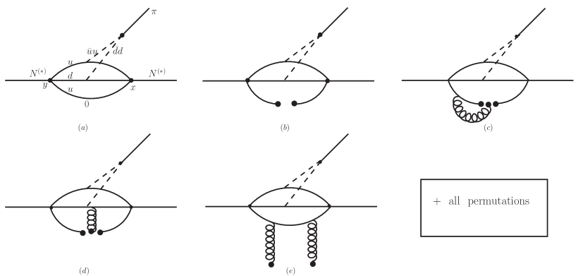
Figure 1: Typical diagrams taken into account in the calculations.

The OPE side in coordinate space is obtained by inserting the above propagator into Eq. (10). A Fourier transformation is applied to transform the calculations to the momentum space. To this end, the following expression in $D$ dimension is used:

$$\frac{1}{[A^{2}]^{n}} = \int\frac{d^{D}t}{(2\pi)^{D}}e^{-it\cdot A}~{}i~{}(-1)^{n+1}~{}2^{D-2n}~{}\pi^{D/2}~{}\frac{\Gamma(D/2-n)}{\Gamma(n)}\Big{(}-\frac{1}{t^{2}}\Big{)}^{D/2-n},$$ (12)

and the four-integrals over $x$ and $y$ are performed after the replacements $x_{\mu}\rightarrow i\frac{\partial}{\partial p_{\mu}}$ and $y_{\mu}\rightarrow-i\frac{\partial}{\partial p^{\prime}_{\mu}}$. After making use of the Feynman parametrization and the equation

$$\int d^{4}t\frac{(t^{2})^{\beta}}{(t^{2}+L)^{\alpha}}=\frac{i\pi^{2}(-1)^{\beta-\alpha}\Gamma(\beta+2)\Gamma(\alpha-\beta-2)}{\Gamma(2)\Gamma(\alpha)[-L]^{\alpha-\beta-2}},$$ (13)

we get

$$\Pi^{OPE}(q) = \Pi_{1}(q^{2})\not\!p\not\!q\gamma_{5}+\Pi_{2}(q^{2})\not\!p\gamma_{5}+\Pi_{3}(q^{2})\not\!q\gamma_{5}+\Pi_{4}(q^{2})\gamma_{5},$$ (14)

where the functions $\Pi_{i}(q^{2})$ include the contributions coming from both the perturbative and non-perturbative parts. These functions are given as

$$\Pi_{i}(q^{2})=\int ds\int ds^{\prime}\frac{\rho_{i}^{pert}(s,s^{\prime},q^{2})+\rho_{i}^{non-pert}(s,s^{\prime},q^{2})}{(s-p^{2})(s^{\prime}-p^{\prime^{2}})}~{},$$ (15)

where the $\rho_{i}(s,s^{\prime},q^{2})$ appearing in this equation are corresponding to spectral densities associated with different structures. They are attained by taking the imaginary parts of the $\Pi_{i}$ functions, i.e. $\rho_{i}(s,s^{\prime},q^{2})=\frac{1}{\pi}Im[\Pi_{i}]$. As examples, we present only the spectral densities corresponding to the Dirac structure $\gamma_{5}$ here. They are obtained as

$$\rho_{4}^{pert}(s,s^{\prime},q^{2}) = \int_{0}^{1}dx\int_{0}^{1-x}dy\frac{i^{3}}{128\pi^{4}y}(1-\beta)(7\beta+5)\Big{[}q^{4}x(x+y-1)\Big{(}1+x^{2}+x(y-1)$$ (16)

$$- y(1+y)\Big{)}-q^{2}\Big{(}sxy(1-3x+3x^{2}+2xy-y^{2})-s^{\prime}(x+y-1)(y-x-2xy$$

$$+ 3x^{2}y-y^{2}+5xy^{2})\Big{)}+2s^{2}x^{2}y^{2}+ss^{\prime}y(x+4xy-5x^{2}y-5xy^{2})+s^{\prime^{2}}y(x+y-1)$$

$$\times (2y^{2}+xy-y-1)\Big{]}\Theta\Big{[}L_{1}(s,s^{\prime},q^{2})\Big{]},$$

and

$$\rho_{4}^{non-pert}(s,s^{\prime},q^{2}) = \langle\alpha_{s}\frac{G^{2}}{\pi}\rangle\frac{i^{3}}{384\pi^{2}}\Bigg{\{}\int_{0}^{1}dx\int_{0}^{1-x}dy\frac{\beta-1}{y}\Big{[}(5+7\beta)(x^{2}-x+xy)-23y^{2}$$ (17)

$$+ 2y-2y\beta-13y^{2}\beta)\Big{]}\Theta\Big{[}L_{1}(s,s^{\prime},q^{2})\Big{]}+\frac{s^{\prime}(\beta-1)^{2}}{q^{2}}\Theta\Big{[}L_{2}(s,s^{\prime},q^{2})\Big{]}$$

$$+ \frac{s(\beta-1)^{2}}{q^{2}}\Theta\Big{[}L_{3}(s,s^{\prime},q^{2})\Big{]}\Bigg{\}},$$

where

$$L_{1}(s,s^{\prime},q^{2}) = q^{2}(1-x-y)+sxy+s^{\prime}y(1-x-y),$$

$$L_{2}(s,s^{\prime},q^{2}) = s^{\prime}$$

$$L_{3}(s,s^{\prime},q^{2}) = s~{}.$$ (18)

Here $\Theta[...]$ is the unit-step function. For simplicity we ignored to present the terms containing the light quark mass in these formulas.

Now, we match the two sides in Borel scheme, after which we get four equations with nine couplings as unknowns. Hence, we need five more equations to solve nine equations with nine unknowns. We construct these extra equations by applying derivatives with respect to inverse of the Borel mass squares. As a result, we get the following expressions for the strong couplings that we are interested in their calculations in the present work:

$$g_{NN\pi}(q^{2}) = \frac{(m_{u}+m_{d})(m_{\pi}^{2}-q^{2})}{f_{\pi}\lambda_{N}^{2}m_{\pi}^{2}(m_{N}+m_{N^{*}})^{2}(m_{N}-m_{N^{\prime}})^{2}}e^{\frac{m_{N}^{2}}{M^{2}}+\frac{m_{N}^{2}}{M^{\prime^{2}}}}\left\{-m_{N^{*}}\frac{d(\widehat{\textbf{B}}\Pi_{2})}{d\frac{1}{M^{\prime^{2}}}}\right.$$

$$+ \left.\frac{d(\widehat{\textbf{B}}\Pi_{4})}{d\frac{1}{M^{2}}}+m_{N}^{2}\left[\frac{d(\widehat{\textbf{B}}\Pi_{1})}{d\frac{1}{M^{2}}}-m_{N^{*}}\widehat{\textbf{B}}\Pi_{3}+m_{N^{\prime}}(m_{N^{*}}\widehat{\textbf{B}}\Pi_{1}+\widehat{\textbf{B}}\Pi_{3})\right]+m_{N^{*}}^{2}\widehat{\textbf{B}}\Pi_{4}\right.$$

$$+ \left.q^{2}\frac{d(\widehat{\textbf{B}}\Pi_{1})}{d\frac{1}{M^{2}}}+q^{2}m_{N^{*}}^{2}\widehat{\textbf{B}}\Pi_{1}-m_{N^{\prime}}^{2}\left[m_{N^{*}}^{2}\widehat{\textbf{B}}\Pi_{1}+m_{N^{*}}\widehat{\textbf{B}}\Pi_{3}-\widehat{\textbf{B}}\Pi_{4}-q^{2}\widehat{\textbf{B}}\Pi_{1}\right]\right.$$

$$- \left.m_{N}\left[-\frac{d(\widehat{\textbf{B}}\Pi_{2})}{d\frac{1}{M^{2}}}+m_{N^{*}}^{2}(\widehat{\textbf{B}}\Pi_{2}+\widehat{\textbf{B}}\Pi_{3})+m_{N^{\prime}}^{2}(m_{N^{*}}\widehat{\textbf{B}}\Pi_{1}+\widehat{\textbf{B}}\Pi_{2}+\widehat{\textbf{B}}\Pi_{3})\right.\right.$$

$$+ \left.\left.m_{N^{\prime}}\left(2\frac{d(\widehat{\textbf{B}}\Pi_{1})}{d\frac{1}{M^{\prime^{2}}}}-\frac{d(\widehat{\textbf{B}}\Pi_{1})}{d\frac{1}{M^{2}}}-m_{N^{*}}^{2}\widehat{\textbf{B}}\Pi_{1}-3m_{N^{*}}\widehat{\textbf{B}}\Pi_{2}-2m_{N^{*}}\widehat{\textbf{B}}\Pi_{3}+\widehat{\textbf{B}}\Pi_{4}\right.\right.\right.$$

$$+ \left.\left.\left.q^{2}\widehat{\textbf{B}}\Pi_{1}\right)+m_{N^{*}}\left(\frac{d(\widehat{\textbf{B}}\Pi_{1})}{d\frac{1}{M^{2}}}-2\frac{d(\widehat{\textbf{B}}\Pi_{1})}{d\frac{1}{M^{\prime^{2}}}}-\widehat{\textbf{B}}\Pi_{4}-q^{2}\widehat{\textbf{B}}\Pi_{1}\right)\right]+m_{N^{\prime}}\left[\frac{d(\widehat{\textbf{B}}\Pi_{2})}{d\frac{1}{M^{\prime^{2}}}}\right.\right.$$

$$+ \left.\left.m_{N^{*}}\left(-\frac{d(\widehat{\textbf{B}}\Pi_{1})}{d\frac{1}{M^{2}}}+m_{N^{*}}\widehat{\textbf{B}}\Pi_{3}-\widehat{\textbf{B}}\Pi_{4}-q^{2}\widehat{\textbf{B}}\Pi_{1}\right)\right]\right\},$$

$$g_{N^{*}N\pi}(q^{2}) = \frac{(m_{u}+m_{d})(m_{\pi}^{2}-q^{2})}{f_{\pi}m_{\pi}^{2}\lambda_{N}\lambda_{N^{*}}(m_{N}+m_{N^{*}})^{2}(m_{N}-m_{N^{\prime}})(m_{N^{\prime}}+m_{N^{*}})}e^{\frac{m_{N^{*}}^{2}}{M^{2}}+\frac{m_{N}^{2}}{M^{\prime^{2}}}}$$

$$\times \left\{m_{N^{\prime}}\left(m_{N^{*}}\frac{d(\widehat{\textbf{B}}\Pi_{1})}{d\frac{1}{M^{\prime^{2}}}}+\frac{d(\widehat{\textbf{B}}\Pi_{2})}{d\frac{1}{M^{\prime^{2}}}}-m_{N^{*}}\frac{d(\widehat{\textbf{B}}\Pi_{1})}{d\frac{1}{M^{2}}}\right)+\frac{d(\widehat{\textbf{B}}\Pi_{4})}{d\frac{1}{M^{2}}}+m_{N}^{2}m_{N^{*}}\widehat{\textbf{B}}\Pi_{2}\right.$$

$$+ \left.m_{N}^{2}\left(\frac{d(\widehat{\textbf{B}}\Pi_{1})}{d\frac{1}{M^{2}}}-\frac{d(\widehat{\textbf{B}}\Pi_{1})}{d\frac{1}{M^{\prime^{2}}}}-m_{N^{\prime}}\widehat{\textbf{B}}\Pi_{2}\right)+m_{N}\left[m_{N^{*}}\frac{d(\widehat{\textbf{B}}\Pi_{1})}{d\frac{1}{M^{\prime^{2}}}}+\frac{d(\widehat{\textbf{B}}\Pi_{2})}{d\frac{1}{M^{\prime^{2}}}}\right.\right.$$

$$- \left.\left.m_{N^{*}}\frac{d(\widehat{\textbf{B}}\Pi_{1})}{d\frac{1}{M^{2}}}+\frac{d(\widehat{\textbf{B}}\Pi_{2})}{d\frac{1}{M^{2}}}+m_{N^{\prime}}\left(\frac{d(\widehat{\textbf{B}}\Pi_{1})}{d\frac{1}{M^{2}}}-\frac{d(\widehat{\textbf{B}}\Pi_{1})}{d\frac{1}{M^{\prime^{2}}}}+2m_{N^{*}}\widehat{\textbf{B}}\Pi_{2}\right)\right]\right.$$

$$+ \left.q^{2}\frac{d(\widehat{\textbf{B}}\Pi_{1})}{d\frac{1}{M^{2}}}+m_{N^{\prime}}^{2}\left(m_{N^{*}}\widehat{\textbf{B}}\Pi_{2}+\widehat{\textbf{B}}\Pi_{4}+q^{2}\widehat{\textbf{B}}\Pi_{1}\right)\right\},$$

$$g_{NN^{*}\pi}(q^{2}) = \frac{(m_{u}+m_{d})(m_{\pi}^{2}-q^{2})}{f_{\pi}m_{\pi}^{2}\lambda_{N}\lambda_{N^{*}}(m_{N}+m_{N^{*}})^{2}(m_{N}-m_{N^{\prime}})(m_{N^{\prime}}+m_{N^{*}})}e^{\frac{m_{N}^{2}}{M^{2}}+\frac{m_{N^{*}}^{2}}{M^{\prime^{2}}}}$$

$$\times \left\{m_{N^{*}}^{2}\frac{d(\widehat{\textbf{B}}\Pi_{1})}{d\frac{1}{M^{\prime^{2}}}}+m_{N^{*}}\frac{d(\widehat{\textbf{B}}\Pi_{2})}{d\frac{1}{M^{\prime^{2}}}}-m_{N^{*}}^{2}\frac{d(\widehat{\textbf{B}}\Pi_{1})}{d\frac{1}{M^{2}}}+m_{N^{*}}\frac{d(\widehat{\textbf{B}}\Pi_{2})}{d\frac{1}{M^{2}}}-\frac{d(\widehat{\textbf{B}}\Pi_{4})}{d\frac{1}{M^{2}}}\right.$$

$$+ \left.m_{N}(m_{N^{\prime}}-m_{N^{*}})\left(\frac{d(\widehat{\textbf{B}}\Pi_{1})}{d\frac{1}{M^{\prime^{2}}}}-\frac{d(\widehat{\textbf{B}}\Pi_{1})}{d\frac{1}{M^{2}}}+m_{N^{\prime}}\widehat{\textbf{B}}\Pi_{2}-m_{N^{*}}\widehat{\textbf{B}}\Pi_{2}\right)\right.$$

$$- \left.m_{N^{\prime}}\left(m_{N^{*}}\frac{d(\widehat{\textbf{B}}\Pi_{1})}{d\frac{1}{M^{\prime^{2}}}}+\frac{d(\widehat{\textbf{B}}\Pi_{2})}{d\frac{1}{M^{\prime^{2}}}}-m_{N^{*}}\frac{d(\widehat{\textbf{B}}\Pi_{1})}{d\frac{1}{M^{2}}}-m_{N^{*}}^{2}\widehat{\textbf{B}}\Pi_{2}\right)\right.$$

$$- \left.q^{2}\frac{d(\widehat{\textbf{B}}\Pi_{1})}{d\frac{1}{M^{2}}}-m_{N^{\prime}}^{2}(\widehat{\textbf{B}}\Pi_{4}+q^{2}\widehat{\textbf{B}}\Pi_{1})\right\},$$

$$g_{N^{*}N^{*}\pi}(q^{2}) = \frac{(m_{u}+m_{d})(m_{\pi}^{2}-q^{2})}{f_{\pi}m_{\pi}^{2}\lambda_{N^{*}}^{2}(m_{N}+m_{N^{*}})^{2}(m_{N^{*}}+m_{N^{\prime}})^{2}}e^{\frac{m_{N^{*}}^{2}}{M^{2}}+\frac{m_{N^{*}}^{2}}{M^{\prime^{2}}}}$$

$$\times \left\{-m_{N^{*}}^{2}\frac{d(\widehat{\textbf{B}}\Pi_{1})}{d\frac{1}{M^{2}}}+m_{N^{*}}\frac{d(\widehat{\textbf{B}}\Pi_{2})}{d\frac{1}{M^{2}}}-\frac{d(\widehat{\textbf{B}}\Pi_{4})}{d\frac{1}{M^{2}}}-q^{2}\frac{d(\widehat{\textbf{B}}\Pi_{1})}{d\frac{1}{M^{2}}}-m_{N^{\prime}}^{2}\widehat{\textbf{B}}\Pi_{4}\right.$$

$$- \left.m_{N^{\prime}}^{2}\left[m_{N^{*}}\left(\widehat{\textbf{B}}\Pi_{2}+\widehat{\textbf{B}}\Pi_{3}\right)+q^{2}\widehat{\textbf{B}}\Pi_{1}\right]+m_{N}^{2}\left[m_{N^{\prime}}^{2}\widehat{\textbf{B}}\Pi_{1}+m_{N^{\prime}}\left(m_{N^{*}}\widehat{\textbf{B}}\Pi_{1}-\widehat{\textbf{B}}\Pi_{3}\right)\right.\right.$$

$$- \left.\left.m_{N^{*}}\left(\widehat{\textbf{B}}\Pi_{2}+\widehat{\textbf{B}}\Pi_{3}\right)-\widehat{\textbf{B}}\Pi_{4}-q^{2}\widehat{\textbf{B}}\Pi_{1}\right]-m_{N^{\prime}}\left[\frac{d(\widehat{\textbf{B}}\Pi_{2})}{d\frac{1}{M^{\prime^{2}}}}+m_{N^{*}}^{2}\widehat{\textbf{B}}\Pi_{3}+m_{N^{*}}\right.\right.$$

$$\times \left.\left.\left(2\frac{d(\widehat{\textbf{B}}\Pi_{1})}{d\frac{1}{M^{\prime^{2}}}}-\frac{d(\widehat{\textbf{B}}\Pi_{1})}{d\frac{1}{M^{2}}}+\widehat{\textbf{B}}\Pi_{4}+q^{2}\widehat{\textbf{B}}\Pi_{1}\right)\right]+m_{N}\left[-\frac{d(\widehat{\textbf{B}}\Pi_{2})}{d\frac{1}{M^{\prime^{2}}}}+m_{N^{*}}^{2}m_{N^{\prime}}\widehat{\textbf{B}}\Pi_{1}\right.\right.$$

$$- \left.\left.m_{N^{*}}^{2}\widehat{\textbf{B}}\Pi_{3}-m_{N^{\prime}}\left(\frac{d(\widehat{\textbf{B}}\Pi_{1})}{d\frac{1}{M^{2}}}+m_{N^{\prime}}\widehat{\textbf{B}}\Pi_{3}+\widehat{\textbf{B}}\Pi_{4}+q^{2}\widehat{\textbf{B}}\Pi_{1}\right)+m_{N^{*}}\frac{d(\widehat{\textbf{B}}\Pi_{1})}{d\frac{1}{M^{2}}}\right.\right.$$

$$- \left.\left.m_{N^{*}}\left(2\frac{d(\widehat{\textbf{B}}\Pi_{1})}{d\frac{1}{M^{\prime^{2}}}}-m_{N^{\prime}}^{2}\widehat{\textbf{B}}\Pi_{1}+3m_{N^{\prime}}\widehat{\textbf{B}}\Pi_{2}+2m_{N^{\prime}}\widehat{\textbf{B}}\Pi_{3}+\widehat{\textbf{B}}\Pi_{4}+q^{2}\widehat{\textbf{B}}\Pi_{1}\right)\right]\right\},$$

where $\widehat{\textbf{B}}\Pi_{i}$ show the Borel transformed form of $\Pi_{i}$ functions and $\frac{d(\widehat{\textbf{B}}\Pi_{i})}{d\frac{1}{M^{(^{\prime})2}}}$ are their derivatives with respect to inverse of the Borel mass squares. We also apply the continuum subtraction in the initial and final channels in this step and this add two more auxiliary parameters $s_{0}$ and $s^{\prime}_{0}$ that they should also be fixed.

3 Numerical results

This section contains the numerical analysis and our discussion on the dependence of the results on $Q^{2}=-q^{2}$. The numerical analysis requires some input parameters given in table 1. From the sum rules for the coupling constants it is also clear that we need to know the residues of $N$ and $N^{*}$ baryons. We use their $\beta$-dependent expressions calculated in Ref. [10] adding also the contribution of $N(1440)$ to the mass sum rules.

Parameters	Values
$\langle\frac{\alpha_{s}G^{2}}{\pi}\rangle$	$(0.012\pm 0.004)$  GeV4 [31]
$m_{d}$	$4.8^{+0.5}_{-0.3}~{}\mbox{MeV}$[32]
$m_{u}$	$2.3^{+0.7}_{-0.5}~{}\mbox{MeV}$ [32]
$m_{N}$	$(938.272046\pm 0.000021)~{}\mbox{MeV}$ [32]
$m_{N^{*}}$	$1525~{}TO~{}1535~{}\mbox{MeV}$ [32]
$m_{\pi}$	$(134.9766\pm 0.0006)~{}\mbox{MeV}$ [32]
$f_{\pi}$	$(130.41\pm 0.03\pm 0.20)~{}\mbox{MeV}$ [33]

Table 1: Input parameters used in the calculations.

In addition to the input parameters given in the table 1 there are four parameters, $M^{2}$, $M^{\prime 2}$, $s_{0}$ and $s^{\prime}_{0}$ that should be fixed. By virtue of being auxiliary parameters, the results should practically be independent of them as much as possible. This necessitates a search for working regions of these parameters. Considering the relations with the first excited states in the initial and final channels, that is, the energy that characterizes the beginning of the continuum; as well as the fact that the sum rules obtained contain all three states in the physical sides, we determine that the suitable interval for both continuum thresholds is $(2.64-2.74)~{}GeV^{2}$. As for the Borel mass parameters, the analysis are done over the criteria that the contributions of the higher states and continuum are sufficiently suppressed and the contributions of the operators with higher dimensions are small. Our analysis based on these criteria leads to the intervals $(1.0-3.0)~{}GeV^{2}$ and $(2.0-4.0)~{}GeV^{2}$ for the Borel parameters in the $N$ and $N^{*}$ channels, respectively.

As already mentioned, in our calculations, we use the most general form of the interpolating field for nucleon which is composed of two independent interpolating fields connected by a mixing parameter $\beta$. In the analysis, we need the values of this auxiliary parameter for which we have weak dependence of the results on this parameter. Our numerical analysis shows that in the intervals $-1\leq cos\theta\leq-0.5$ and $0.5\leq cos\theta\leq 1$, common for all vertices, the results depend weakly on this parameter. Note that we use $\cos\theta$ where $\theta=\tan^{-1}(\beta)$ to explore the whole range ($-\infty$, $+\infty$) for $\beta$ via $-1\leq\cos\theta\leq 1$. Considering the maximum contribution of the ground state pole to the sum rules, we found that $\cos\theta=-0.6$, common for all vertices, is roughly the optimum value that leads to the largest $pole/total~{}contribution$ ratio. We use this value to extract the values of the coupling constants under consideration. We shall note that by the above working regions for the continuum thresholds and Borel parameters as well as the value of $\cos\theta$, not only the pole contribution is maximum ($\simeq 70\%$ of the total contribution), but also the series of sum rules properly converge, i.e., the perturbative part constitutes roughly $78\%$ and the term with higher dimension constitutes less than $5\%$ of the pole contribution.

In this part we would like to show how the results of strong coupling constants depend on the Borel parameters. To this end, we plot the dependence of $g_{NN^{*}\pi}$, as an example, on these parameters at the average values of the continuum thresholds, $\cos\theta=-0.6$ and $Q^{2}=1GeV^{2}$ in figure 2. From this figure we see that the results weakly depend on the Borel parameters in their working interval.

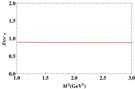
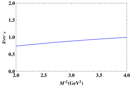
Figure 2: Left: $g_{NN^{*}\pi}$ as a function of $M^{2}$ at average values of continuum thresholds, $\cos\theta=-0.6$, $Q^{2}=1GeV^{2}$ and $M^{{}^{\prime}2}=3GeV^{2}$. Right: $g_{NN^{*}\pi}$ as a function of $M^{{}^{\prime}2}$ at average values of continuum thresholds, $\cos\theta=-0.6$, $Q^{2}=1GeV^{2}$ and $M^{2}=2GeV^{2}$

Now, we proceed to discuss the behavior of the coupling constants with respect to $Q^{2}$. Our calculations show that the following fit function describes well the strong couplings under consideration:

$$g_{N^{(*)}N^{(*)}\pi}(Q^{2})=\frac{f_{0}}{1-a\frac{Q^{2}}{m_{N^{(*)}}^{2}}+b\Big{(}\frac{Q^{2}}{m_{N^{(*)}}^{2}}\Big{)}^{2}}.$$ (20)

Table 2 presents the values of fit parameters, $f_{0}$, $a$ and $b$, for each coupling form factor. Figures (3) and (4) show the dependence of the strong coupling constants under consideration on $Q^{2}$ for both sum rules and fit results. From these figures, we observe that the above fit function reproduces well the QCD sum rules results up to the truncated points.

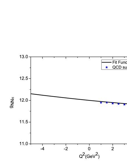
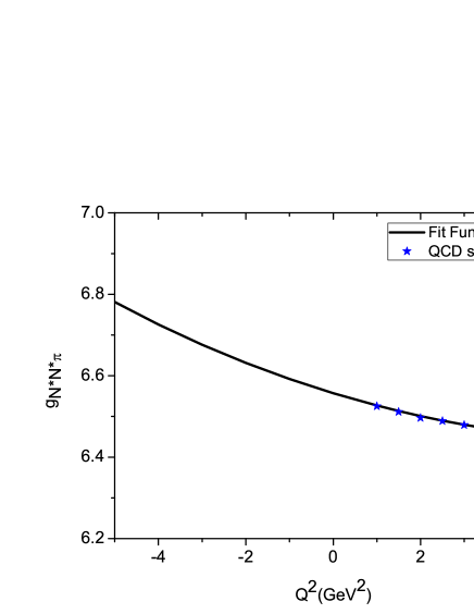
Figure 3: Left: $g_{NN\pi}$ as a function of $Q^{2}$. Right: $g_{N^{*}N^{*}\pi}$ as a function of $Q^{2}$

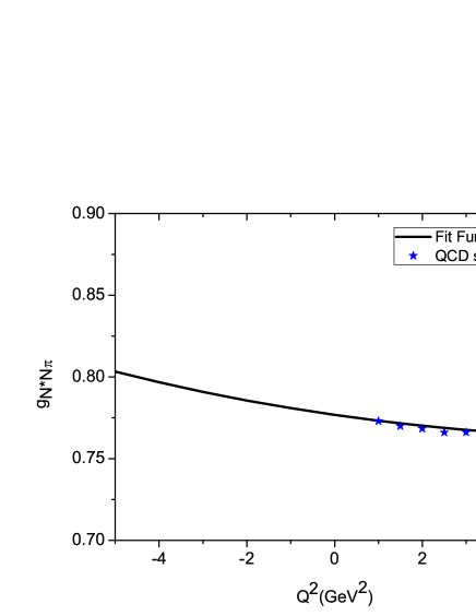
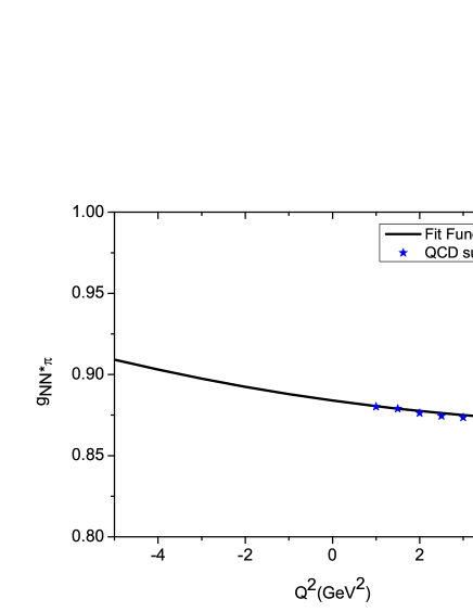
Figure 4: Left: $g_{N^{*}N\pi}$ as a function of $Q^{2}$. Right: $g_{NN^{*}\pi}$ as a function of $Q^{2}$

The usage of the fit function at $Q^{2}=-m_{\pi}^{2}$ leads us to the value of strong coupling constant for each considered transition as presented in table 3 with the errors arising from the uncertainties of the input parameters as well as those coming from the determination of the working regions of the auxiliary parameters. From this table we see that the couplings associated to the $N^{*}N\pi$ and $NN^{*}\pi$ vertices are strongly suppressed compared to those related to two other vertices. The strong coupling $g_{N^{*}N^{*}\pi}$ is obtained to be equal to roughly half of that of $g_{NN\pi}$. From our results we also see that the results for $g_{N^{*}N\pi}$ and $g_{NN^{*}\pi}$ are very close to each other, which is an expected situation. The result obtained for $g_{NN\pi}$ is, within the errors, in good agreement with the results of Refs. [16, 17, 22, 24] that obtain $g_{NN\pi}=12\pm 5$ [16, 17], $g_{NN\pi}=9.76\pm 2.04$ [22] and $g_{NN\pi}=13.3\pm 1.2$ [24]. Our prediction on the $g_{NN^{*}\pi}$ is also consistent with the results of [19, 23] that extract the value   $g_{NN^{*}\pi}\sim 0.7$ from the experimental data, but it differs considerably from the result of [23] which obtains $g_{NN^{*}\pi}=(-)(0.08\pm 0.06)$ from light cone QCD sum rules. Our result on the strong coupling constant $g_{N^{*}N^{*}\pi}$ can be checked via different phenomenological approaches as well as in future experiments.

$$\begin{array}[]{|c|c|c|c|c|c|}\hline\cr\hline\cr\mbox{}&f_{0}&a&b\\ \hline\cr\mbox{$g_{NN\pi}$}&12.001\pm 3.480&-0.005\pm 0.001&(-3.143\pm 0.943)10^{-4}\\ \hline\cr\mbox{$g_{N^{*}N^{*}\pi}$}&6.557\pm 1.961&-0.012\pm 0.003&(-1.821\pm 0.546)10^{-3}\\ \hline\cr\mbox{$g_{N^{*}N\pi}$}&0.777\pm 0.233&-0.012\pm 0.003&(-1.820\pm 0.546)10^{-3}\\ \hline\cr\mbox{$g_{NN^{*}\pi}$}&0.884\pm 0.256&-0.004\pm 0.001&(-2.070\pm 0.621)10^{-4}\\ \hline\cr\hline\cr\end{array}$$

Table 2: Parameters appearing in the fit function.

$$\begin{array}[]{|c|c|c|c|c|}\hline\cr\hline\cr\mbox{$g_{NN\pi}$}&\mbox{$g_{N^{*}N^{*}\pi}$}&\mbox{$g_{N^{*}N\pi}$}&\mbox{$g_{NN^{*}\pi}$}\\ \hline\cr 12.012\pm 3.608&6.564\pm 1.842&0.782\pm 0.233&0.882\pm 0.264\\ \hline\cr\hline\cr\end{array}$$

Table 3: Values of the strong coupling constants.

To sum up, we have calculated the couplings $g_{NN\pi}$, $g_{N^{*}N\pi}$, $g_{NN^{*}\pi}$ and $g_{N^{*}N^{*}\pi}$ using three point QCD sum rules. We used the most general form of the interpolating current for the nucleon. After fixing the auxiliary parameters entering the calculations, we extracted the values of those couplings. We have found that the couplings $g_{N^{*}N\pi}$ and $g_{NN^{*}\pi}$ are strongly suppressed. The value of the coupling constant $g_{N^{*}N^{*}\pi}$ is also obtained to be roughly half of $g_{NN\pi}$. Our results on $g_{NN\pi}$ and $g_{NN^{*}\pi}$ are in agreement with those of [16, 17, 22, 24, 23] which extract the results from different models as well as from the experimental data on the decay width of the corresponding transitions. Our result on $g_{NN^{*}\pi}$ considerably differs from the result of light cone QCD sum rules obtained in [23]. This inconsistency can be attributed to the fact that the masses of the nucleon $N$ and the negative parity $N^{*}$ differ considerably and usage of the light cone QCD sum rules, as is done in [23], for such vertex is problematic. Our prediction on the strong coupling constant $g_{N^{*}N^{*}\pi}$ can be checked via different phenomenological approaches as well as in future experiments.

References

- [1] Y. Chung, H. G. Dosch, M. Kremer and D. Schall, “Baryon Sum Rules and Chiral Symmetry Breaking”, Nucl. Phys. B 197, 55 (1982).
- [2] Frank X. Lee, Derek B. Leinweber, “Negative parity baryon spectroscopy”, Nucl. Phys. Proc. Suppl.73, 258 (1999), hep-lat/9809095.
- [3] Y. Kondo, O. Morimatsu, T. Nishikawa, “Coupled QCD sum rules for positive and negative-parity nucleons”, Nucl. Phys. A 764, 303 (2006), arXiv:hep-ph/0503150.
- [4] D. Jido, M. Oka, A. Hosaka, “Negative parity baryons in the QCD sum rule”, Nucl. Phys. A 629, 156 (1998), arXiv:hep-ph/9702351.
- [5] D. Jido, N. Kodama, M. Oka, “Negative-parity Nucleon Resonance in the QCD Sum Rule” Phys. Rev. D 54, 4532 (1996), arXiv:hep-ph/9604280.
- [6] T. M. Aliev, M. Savci, “Magnetic moments of negative parity baryons in QCD”, Phys. Rev. D 89, 053003 (2014), arXiv:1402.4609 [hep-ph].
- [7] I. M. Narodetskii, M.A. Trusov, “Magnetic Moments of Negative Parity Baryons from Effective Hamiltonian Approach to QCD”, JETP Letters, 99, 57 (2014), arXiv:1311.2407 [hep-ph].
- [8] T. M. Aliev, M. Savci, “ transition form factors in QCD”, Phys. Rev. D 88, 056021 (2013), arXiv:1308.3142 [hep-ph].
- [9] T. M. Aliev, M. Savci, “ transition form factors in light cone QCD sum rules”, Phys. Rev. D 90, 096012 (2014), arXiv:1409.5250 [hep-ph].
- [10] K. Azizi, H. Sundu, “Radiative transition of negative to positive parity nucleon”, Phys.Rev. D91 (2015) 9, 093012, arXiv:1501.07691 [hep-ph]
- [11] T. Meissner, “ form factor from QCD sum rules”, Phys. Rev. C 52, 3386 (1995), arXiv:nucl-th/9506030.
- [12] T. Meissner and E. M. Henley, “Isospin breaking in the pion-nucleon coupling from QCD sum rules”, Phys. Rev. C 55, 3093 (1997), arXiv:nucl-th/9601030.
- [13] T. M. Aliev, A. Ozpineci, M. Savci, “Meson-Baryon Couplings and the F/D ratio in Light Cone QCD”, Phys. Rev. D 64, 034001 (2001), arXiv: hep-ph/0012170.
- [14] Y. Kondo, O. Morimatsu, “Model-independent study of the QCD sum rule for the coupling constant”, Phys. Rev. C 66, 028201 (2002), arXiv: nucl-th/0102028.
- [15] H. Shiomi, T. Hatsuda, “The Pion-Nucleon Coupling Constant in QCD Sum Rules”, Nucl. Phys. A 594, 294 (1995), arXiv: hep-ph/9504354.
- [16] M. C. Birse, B. Krippa, “Determination of the pion-nucleon coupling constant from QCD sum rules”, Phys. Lett. B 373, 9 (1996), arXiv:hep-ph/9512259.
- [17] M. C. Birse and B. Krippa, “Determination of pion-baryon coupling constants from QCD sum rules”, Phys. Rev. C 54, 3240 (1996), arXiv: hep-ph/9606471.
- [18] D. Jido, M. Oka, A. Hosaka, “Suppression of Coupling in the QCD Sum Rule”, arXiv:hep-ph/9610520.
- [19] A. Hosaka, D. Jido, M. Oka, “Suppression of Coupling in the QCD Sum Rule”, arXiv:hep-ph/9702294.
- [20] D. Jido, M. Oka, A. Hosaka, “Suppression of Coupling and Chiral Symmetry”, Phys. Rev. Lett. 80, 448 (1998), arXiv: hep-ph/9707307.
- [21] Hungchong Kim and Su Houng Lee, “Calculation of and couplings in QCD sum rules”, Phys. Rev. D 56, 4278 (1997), arXiv: nucl-th/9704035.
- [22] Hungchong Kim, Su Houng Lee, Makoto Oka, “QCD sum rule calculation of the coupling-revisited”, Phys. Lett. B 453, 199 (1999), arXiv:nucl-th/9809004.
- [23] Shi-Lin Zhu, “The suppression of coupling in QCD”, Mod. Phys. Lett. A 13, 2763 (1998), arXiv: hep-ph/9810255.
- [24] Hungchong Kim, “ coupling determined beyond the chiral limit”, Eur. Phys. J. A 7, 121 (2000).
- [25] Hung-chong Kim, Su Houng Lee, Makoto Oka, “Two-point correlation function with pion in QCD sum rules”, Phys. Rev. D 60, 034007 (1999), arXiv:nucl-th/9904049.
- [26] T. E. O. Ericson, B. Loiseau, A. W. Thomas, “Determination of the pion-nucleon coupling constant and scattering lengths”, Phys. Rev. C 66, 014005 (2002), arXiv: hep-ph/0009312.
- [27] C. Downum, T. Barnes, J. R. Stone, E. S. Swanson, “Nucleon-meson coupling constants and form factors in the quark model”, Phys. Lett. B 638, 455 (2006), arXiv: nucl-th/0603020.
- [28] T. E. O. Ericson, B. Loiseau, J. Rahm, J. Blomgren, N. Olsson, A. W. Thomas, “Precise strength of the coupling constant Olsson”, Nucl. Phys. A 654, 939 (1999), arXiv:hep-ph/9811515.
- [29] M. A. Shifman, A. I. Vainshtein, and V. I. Zakharov, “QCD and resonance physics. Theoretical foundations”,Nucl. Phys. B147, 385 (1979); B147, “QCD and resonance physics. Applications”, 448 (1979).
- [30] L. J. Reinders, H. Rubinstein, S. Yazaki, “Hadron properties from QCD sum rules”, Phys. Rept. 127, 1 (1985).
- [31] V. M. Belyaev, B. L. Ioffe, “Determination Of Baryon And Baryonic Masses From Qcd Sum Rules. Strange Baryons ”, Sov. Phys. JETP 57, 716 (1983); Phys. Lett. B 287, 176 (1992).
- [32] K. A. Olive et al. (Particle Data Group), “Review of Particle Physics” Chin. Phys. C, 38, 090001 (2014).
- [33] J. L. Rosner and S. Stone in J. Beringer et al., Phys. Rev. D 86, 946 (2012)