Minimum Anisotropy of a Magnetic Nanoparticle out of Equilibrium

Abstract

In this article we study magnetotransport in single nanoparticles of Ni, Py=Ni_0.8Fe_0.2, Co, and Fe, with volumes $15\pm 6$nm³, using sequential electron tunneling at 4.2K temperature. We measure current versus magnetic field in the ensembles of nominally the same samples, and obtain the abundances of magnetic hysteresis. The hysteresis abundance varies among the metals as Ni:Py:Co:Fe=4 :50 :100 :100(%), in good correlation with the magnetostatic and magnetocrystalline anisotropy. The abrupt change in the hysteresis abundance among these metals suggests a concept of minimum magnetic anisotropy required for magnetic hysteresis, which is found to be $\approx 13$meV. The minimum anisotropy is explained in terms of the residual magnetization noise arising from the spin-orbit torques generated by sequential electron tunneling. The magnetic hysteresis abundances are weakly dependent on the tunneling current through the nanoparticle, which we attribute to current dependent damping.

Magnetic anisotropy in ferromagnets is vital in magneto-electronic applications, such as giant magnetoresitance Baibich et al. (1988); Grünberg et al. (1986) and spin-transfer torque. Slonczewski (1996); Berger (1996); Ralph and Styles (2008) For example, in some applications, a strong spin-orbit anisotropy is desired in order to establish a hard or fixed reference magnetic layer, while in other applications, it is beneficial to use a weaker anisotropy in order to fabricate an easily manipulated, soft or free magnetic layer. The ability to tune the degree of anisotropy for various applications is therefore of utmost importance. In thermal equilibrium, the minimum anisotropy necessary for magnetic hysteresis is temperature dependent Néel (1949); Brown (1963); Wernsdorfer et al. (1997). In this article, we address the minimum anisotropy in the case of a voltage-biased metallic ferromagnetic nanoparticle First studies of discrete levels and magnetic hysteresis in metallic ferromagnetic nanoparticles have been done on Co nanoparticles Gueron et al. (1999); Deshmukh et al. (2001); Jiang et al. (2013). Here we discuss the magnetic hysteresis abundances in single electron tunneling devices containing similarly sized single nanoparticles of Ni, Py=Ni_0.8Fe_0.2, Co, and Fe. At 4.2K temperature. the probability that a given nanoparticle sample will display magnetic hysteresis in current versus magnetic field, at any bias voltage, was found to vary as follows: Ni:Py:Co:Fe=$0.04$ :$0.5$ :$1$ :$1$. The very small (high) probability of magnetic hysteresis in the Ni (Fe and Co) nanoparticles suggests a concept of minimum magnetic anisotropy necessary for magnetic hysteresis, comparable to the average magnetic anisotropy of Py nanoparticle. The minimum magnetic anisotropy is explained here in terms of the fluctuating spin-orbit torques exerted on the magnetization by sequential electron tunneling. These torques lead to the saturation of the effective magnetic temperature at low temperatures. In order for the nanoparticle to exhibit magnetic hysteresis at 4.2K, the blocking temperature must be larger than the residual temperature. The magnetic hysteresis abundances are found to be independent of the tunneling current through the sample, which suggests that the damping is proportional to the tunneling current.

I Experiment

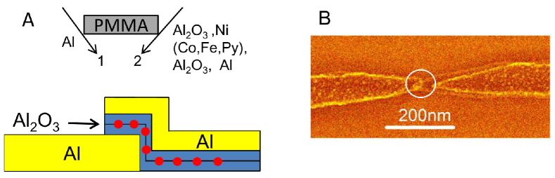
Figure 1: A: Sketch showing the sample fabrication process. B: Scanning electron micrograph of a typical sample.

Our samples consist of similarly-sized ferromagnetic nanoparticles tunnel-coupled to two Al leads via amorphous aluminum oxide barriers. First, a polymethilmetachryllate bridge is defined by electron-beam lithography on a SiO₂ substrate using a technique developed previously, as sketched in Fig. 1A. Next, we deposit $10$nm of Al along direction 1. Then, we switch the deposition to direction 2, and deposit $1.5$nm of Al₂O₃, $0.5$-$1.2$nm of ferromagnetic material, 1.5nm of Al₂O₃, topped off by $10$nm of Al, followed by liftoff in acetone. The tunnel junction is formed by the small overlap between the two leads as shown in the circled part in Fig. 1B. The nanoparticles are embedded in the matrix of Al₂O₃ in the overlap. The nominal thickness of deposited Co, Ni, and Py is $0.5$-$0.6$nm. At that thickness, the deposited metals form isolated nanoparticles approximately $1-5$nm in diameter. We find that if we deposit Fe at the nominally thickness $0.6$nm, then the resulting samples are generally insulating. Thus, the deposited Fe thickness is increased to $1-1.2$nm, which yields samples in the same resistance range as in samples of Co, Ni, and Py. We suppose that because Fe can be easily oxidized, Fe nanoparticles are surrounded by iron oxide shells. Thus, our sample characterization suggests that it is appropriate to attribute the difference among Co, Ni, and Py samples to intrinsic material effects rather than size discrepancies, while, in Fe nanoparticles, the comparison is complicated by the uncertainty in the size of the metallic core. Still, we find the comparison with Fe to be fair, because of the wide range of nanoparticle diameters involved.

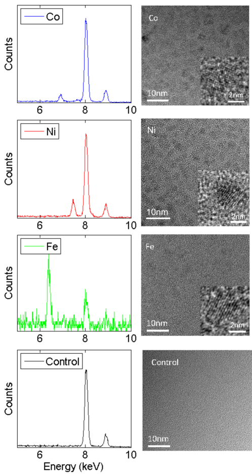
Figure 2: EDS spectra and TEM images of aluminum oxide surface topped with 0.6nm of Co (top row), 0.6nm of Ni (second row), 1.2nm of Fe (third row), and control Al₂O₃ on TEM grid (bottom row).

We obtain the transmission electron microscope (TEM) image of the deposited pure aluminum oxide surface, and the aluminum oxide surface topped with nominally 1.2nm of Fe, $0.55$nm of Ni, and $0.6$nm of Co, as shown in Fig. 2. The deposition is done immediately prior to loading the sample in the TEM. Pure aluminum oxide surface appears completely amorphous, with no visible signs of crystalline structure. In comparison, single crystal structure can be identified in the TEM images for Fe, Ni, and Co. From the TEM image, the areal coverage of Ni nanoparticles is $44$% and the nanoparticle density is $3.6\cdot 10^{4}\mu$m^-2. Assuming that the nanoparticles have pancake shape, the average area and the height of the particles are $0.44/3.6\cdot 10^{4}\mu$m${}^{-2}\approx 12$nm² and $0.55$nm$/0.44=1.25$nm, respectively. The standard deviation of the nanoparticle s area is $40$% of the average area, which is estimated by the shape analysis in $120$ Ni neighboring nanoparticles. Thus, the volume of the Ni nanoparticles is $15\pm 6$nm³, where $6$nm³ is the standard deviation. The volume distribution in Co nanoparticles is similar to that in Ni. We take the energy dispersive x-ray spectroscopy (EDS) for the samples we imaged, which confirms the materials deposited on the aluminum oxide surface.

II Measurements

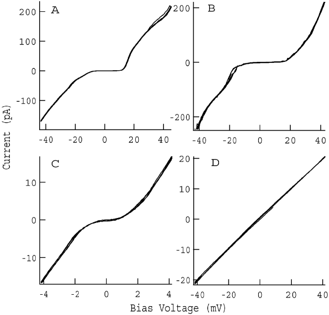
Figure 3: Current versus voltage in four representative samples at 4.2K temperature.A.Co, B.Ni, C.Fe nanoparticles, and D.Leaky pure Al₂O₃ tunneling junctions.

The IV curves are measured using an Ithaco model 1211 current preamplifier and are reproducible with voltage sweeps. Figures 3 A, B, and C display the IV curves of three representative tunneling junctions with embedded nanoparticles of Co, Fe, and Ni, respectively, in samples immersed in liquid Helium at 4.2K. The IV curves display Coulomb blockade (CB) which confirms electron tunneling via metallic nanoparticles, but no discrete levels are resolved. We also measure tunneling junctions containing only the aluminum oxide, without embedded metallic nanoparticles. Those junctions are generally insulating but some are not, e.g., there may be leakage. The IV curves of those leaky junctions are linear, as shown in Fig. 3D, as expected for simple tunnel junctions. We show the IV curve in a pure aluminum oxide junction, to demonstrate that the CB in the samples with embedded metallic nanoparticles originate from tunneling via those nanoparticles. The issue here is that, as will be shown immediately below, some of the samples with embedded nanoparticles do not display any hysteresis in current versus magnetic field at 4.2K. Since those samples also display Coulomb blockade in the I-V curve, we can conclude that the absence of hysteresis is intrinsic to the nanoparticles, rather than an artifact from tunneling through a possibly leaky aluminum oxide.

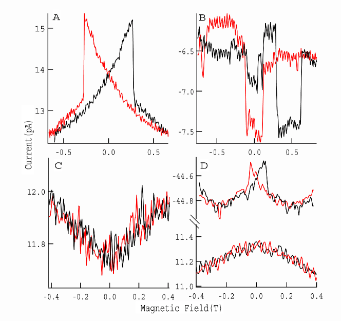
Figure 4: Examples of tunneling current versus magnetic field at 4.2K, for samples with A.Co, B.Fe, C.Ni, and D.Py nanoparticles. In D, two pairs of curves correspond to two different samples. Red(black) lines correspond to decreasing(increasing) magnetic field.

Current versus applied magnetic field (parallel to the film plane) is obtained by measuring the current at a fixed bias voltage while sweeping the magnetic field slowly. Fig. 4A-D show the representative magnetic hysteresis loops for Co, Fe, Ni, and Py samples at 4.2K, respectively. As seen in Fig. 4C and D, the Ni-nanoparticle and one Py nanoparticle have no magnetic hysteresis. All the samples that lack hysteresis do so at the lowest resolved tunneling current. The statistics of the presence of hysteresis for different materials are displayed in Table. 1. All the Co (over 50) and Fe (6), one half of the Py (out of 10), and only 2 of the 46 measured Ni samples, with the switching field $0.05$T and $0.12T$, display magnetic hysteresis. The abrupt change in the hysteresis abundance between Co, Fe, Py, and Ni suggests a concept of minimum magnetic anisotropy necessary for magnetic hysteresis, akin to the concept of Mott’s maximum metallic resistivity. Note that the Ni samples and the non-hysteretic Py samples still display significant magneto-resistance. Among the hysteretic samples, the average magnetic switching field varies as Ni:Py:Co:Fe=$0.085$ :$0.114$ :$0.233$ :$0.257$ (Tesla).

Table 1: Hysteresis percentage versus magnetic anisotropy in different materialsPapaconstantopoulos (1986); Kittel (2004)

Material	Hysteresis($\%$)	$K_{s}$($\mu$eV/spin)	$K1$($\mu$eV/spin)	$K2$($\mu$eV/spin)	$E_{B}$(meV)
CoPaige et al. (1984)	100	105	64.1	8.3	$97\pm 39$
FeTung et al. (1982)	100	128	4.0	1.3	$51\pm 20$
PyMartinez et al. (2006)	50	67.1	0	0	$13\pm 5$
NiGadsden and Heath (1976)	4	37.9	-24.4	4.1	$7.7\pm 3$

The magnetic energy $E_{M}(\vec{m})$ of the Fe/Ni/Py and Co nanoparticles can be written as $S_{0}[K_{1}(m_{x}^{2}m_{y}^{2}+m_{y}^{2}m_{z}^{2}+m_{z}^{2}m_{x}^{2})+K_{2}m_{x}^{2}m_{y}^{2}m_{z}^{2}+K_{s}\vec{m}\hat{N}\vec{m}]$ and $S_{0}[K_{1}m_{z}^{2}+K_{2}m_{z}^{4}+K_{s}\vec{m}\hat{N}\vec{m}]$, respectively, where $S_{0}\hbar$ is the total spin in the nanoparticle, $\vec{m}$ is the magnetization unit vector, and $\hat{N}$ is the demagnetization tensor which is set to have 3 eigenvalues equal to 0.2, 0.3, and 0.5. In the calculations, Euler angles between the principal axes of shape anisotropy and magnetocrystalline anisotropy axes are all equal to $\pi/5$. The results of the calculation of the energy barrier $E_{B}$ are shown in table 1, assuming the nanoparticle average volume obtained in Sec. 2. The error bar reflects the standard deviation in the nanoparticle volume. The abrupt change in magnetic hysteresis abundance is monotonic with the calculated $E_{B}$. Since 50% of Py nanoparticles display hysteresis, it follows that the minimum anisotropy energy barrier required for magnetic hysteresis in our samples at 4.2K is $\approx$13meV. This energy barrier is too large to explain our findings in terms of the reduction in the blocking temperature among these metals. Experimentally, the magnetometry on similarly-sized nanoparticles show that the blocking temperature varies between $13-30$K for Co and $6-20$K for Ni. Sarkar et al. (2005); Luis et al. (2002); Yoon et al. (2005); Galvez et al. (2006); Fonseca et al. (2002) Though Co nanoparticles appear to have higher blocking temperature than Ni nanoparticles, the difference in blocking temperature is not sufficient to explain the vast contrast in the hysteresis abundance in our nanoparticles under electron transport. Theoretically, the Arrhenius flipping rate can be estimated as $\nu_{at}\exp(-E_{B}/k_{B}T)$. Assuming $\nu_{at}=10^{10}$Hz, we obtain the magnetization flipping time of 100 hours, much longer than the time it takes to measure a magnetic hysteresis loop. We conclude that the breakdown in magnetic hysteresis we observe reflects the effect of sequential electron tunneling through the nanoparticle on magnetization. This effect will be discussed in Sec. 4.

III Numerical Simulations

The magnetic Hamiltonian for Ni and Fe nanoparticles can be written as

$$\mathcal{H}(n,\vec{S_{n}}) =S_{0}[\frac{K_{1,n}}{2}(\alpha^{2}\beta^{2}+\beta^{2}\alpha^{2}+\alpha^{2}\gamma^{2}+\gamma^{2}\alpha^{2}+\beta^{2}\gamma^{2}+\gamma^{2}\beta^{2})+\frac{K_{2,n}}{6}(\alpha^{2}\beta^{2}\gamma^{2}$$

$$+\alpha^{2}\gamma^{2}\beta^{2}+\beta^{2}\alpha^{2}\gamma^{2}+\beta^{2}\gamma^{2}\alpha^{2}+\gamma^{2}\beta^{2}\alpha^{2}+\gamma^{2}\alpha^{2}\beta^{2})]-K_{s}\vec{S_{n}}\hat{N}\vec{S_{n}}$$

Co has uniaxial magnetocrystalline anisotropy, thus the magnetic Hamiltonian is

$$\mathcal{H}(n,\vec{S_{n}}) =-S_{0}[K_{1,n}\gamma^{2}+K_{2,n}\gamma^{4}]-K_{s}\vec{S_{n}}\hat{N}\vec{S_{n}}$$

Here, $n$ is the number of electrons in the nanoparticle while $S_{0}\hbar$ is the total spin. $K_{1,n}$, $K_{2,n}$, and $K_{s}$ represent magnetocrystalline anisotropy constants and the shape anisotropy constant per spin, respectively. $\alpha$,$\beta$,$\gamma$=$S_{x}$,$S_{y}$,$S_{z}/S_{0}$. $\hat{N}$ is the demagnetization tensor. The magnetocrystalline anisotropy constants per unit volume $K_{1,V}$ and $K_{2,V}$ are obtained from Refs. Tung et al., 1982; Paige et al., 1984; Martinez et al., 2006; Gadsden and Heath, 1976 . We obtain $2S_{0}/N_{a}$ from Ref. Papaconstantopoulos (1986), where $N_{a}$ is the total number of atoms in the nanoparticle. Then, $S_{0}/V=\rho S_{0}/N_{a}M_{A}$, where $\rho$ is the mass density and $M_{A}$ is the atomic mass. The average value of the magnetocrystalline anisotropy constants per spin $(K_{1},K_{2})$ are $(K_{1,V},K_{2,V})V/S_{0}$, respectively, while, $K_{s}=\mu_{0}M_{s}^{2}V/2S_{0}$, where $M_{s}$ is the saturation magnetization obtained in Ref. Kittel, 2004; Martinez et al., 2006. Because of spin-orbit anisotropy fluctuations, ($K_{1,n},K_{2,n}$) fluctuate around $(K_{1},K_{2})$, respectively, according to the number of electrons $n$. We expect that the average magnetic anisotropy has strong material dependence, while the mesoscopic fluctuations in the total magnetic anisotropy energy due to single electron tunneling on/off, are independent of the material. Cehovin et al. (2002); Usaj and Baranger (2005); Brouwer and Gorokhov (2005) In Co nanoparticles, the change in total magnetic energy after electron tunneling-on is $S_{0}\Delta K\sim 0.4$meV.Usaj and Baranger (2005) In Ni nanoparticles of the same size at 4.2K or below, $S_{0}$ and $K$ are both $\approx 1/3$ of the values in Co nanoparticles. So, the relative fluctuations in magnetic anisotropy $\Delta K/K$ in Ni nanoparticles are enhanced $9-10$ times compared to Co nanoparticles with the same size. At the same time, the magnetic energy barrier in Ni nanoparticles is suppressed because of the cubic symmetry and weak shape anisotropy. As a result, the magnetization in Ni nanoparticles is significantly more susceptible to perturbation by electron transport compared to Co or Fe nanoparticles.

The numerical simulation of the magnetization dynamics is based on the master equation modified from that in Ref. Parcollet and Waintal (2006). In the sequential tunneling regime, the number of electrons in the nanoparticle hops between $n$ and $n+1$. Assuming the electron tunnels through only one minority single electron state $j$, which reduces the spin of the nanoparticle by $1/2$ after the electron tunneling-on event (including more electron states does not affect the result in a major way), the master equation can be written as

$$\begin{split}\frac{\partial P_{\alpha}}{\partial t}=&\sum_{\alpha^{\prime}}\sum_{l=L,R}\sum_{\sigma=\uparrow,\downarrow}\Gamma_{l\sigma}\left\{\left|<\alpha^{\prime}|c_{j\sigma}|\alpha>\right|^{2}\left[-(1-f_{l}(\Delta E_{M}))P_{\alpha}+f_{l}(\Delta E_{M})P_{\alpha^{\prime}}\right]+\right.\\ &\left.\lvert<\alpha^{\prime}|c^{\dagger}_{j\sigma}|\alpha>\rvert^{2}\left[-f_{l}(-\Delta E_{M})P_{\alpha}+(1-f_{l}(-\Delta E_{M}))P_{\alpha^{\prime}}\right]\right\}+\\ &\Gamma_{B}\sum_{\alpha^{\prime},\epsilon=\pm}\epsilon\left|<\alpha^{\prime}|S_{x}-i\epsilon S_{y}|\alpha>\right|^{2}\left[\rho_{B}(\epsilon\Delta E_{M})n_{B}(\Delta E_{M})P_{\alpha^{\prime}}+\rho_{B}(\epsilon\Delta E_{M})n_{B}(-\Delta E_{M})P_{\alpha}\right]\end{split}$$ (1)

The first part of the master equation describes the magnetic tunneling transitions. Here, $|\alpha>$ and $|\alpha^{\prime}>$ represent magnetic eigenstates of the nanoparticle , i.e., the eigenstate of $\mathcal{H}(n,\vec{S_{n}})$ with $n$ or $n+1$ electrons. $|\alpha>$ and $|\alpha^{\prime}>$ can be obtained as superpositions of the eigenstates of $\hat{S}^{2}$ and $\hat{S_{z}}$, which are the pure spin-states $|S_{0},m>$. $c_{j\sigma}$ ($c^{\dagger}_{j\sigma}$) is the annihilation (creation) operator for an electron with spin $\sigma$ on level $j$. $\Gamma_{l\sigma}$ denotes the tunneling rate to level $j$ through the leads $l=L,R$ for electron with spin $\sigma$ and $f_{l}$ is the Fermi distribution in the leads. $\Delta E_{M}=E_{\alpha}-E_{\alpha^{\prime}}$. $<\alpha^{\prime}|c^{\dagger}_{j\sigma}|\alpha>$ is the tunneling transition matrix element for transition between the initial state $|\alpha>$ and the final state $|\alpha^{\prime}>$. The second part of the master equation describes the magnetic damping due the coupling to the bosonic bath. $\Gamma_{B}$ is the rate related to the damping rate $1/T_{1}$. $\rho_{B}(\Delta E_{M})$ is the spectral density of the boson which is set to be constant because it varies very slowlyParcollet and Waintal (2006). $n_{B}$ is the Bose-distribution function.

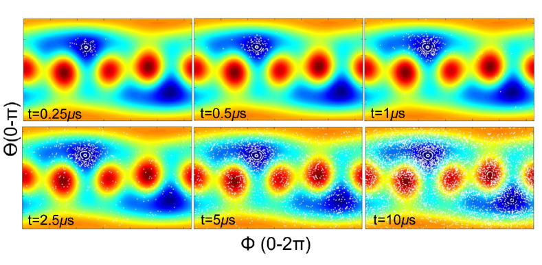
Figure 5: Simulations of the time evolution of the magnetization vector in a Ni nanoparticle. The blue-yellow-red scale indicates the magnetic anisotropy energy landscape from low to high versus the polar angle $\Theta$ and the azimuthal angle $\Phi$ in a Ni nanoparticle. The value of t is the past time counted from the beginning of electron tunneling. The white dots signify possible angle positions at the specified time for each simulation. As time progresses, the likely magnetization position is spread out over phase space and approaches a random isotropic distribution.

Fig. 5 shows the motion of the magnetization statistical distribution versus time. The magnetic anisotropy energy vs ($\Theta,\Phi$) represents the relation between magnetic energy and magnetization direction, where $\Theta,\Phi$ are the two polar angles. Each magnetic state corresponds to a contour on the magnetic anisotropy energy landscape. Classically, one would consider the magnetic state as the magnetization precessing on the contour corresponding to that state. A random dot is selected on a contour to indicate the presence of the magnetic state related to that contour. The number of dots on each contour is decided by the probability of the corresponding magnetic state. The plotted dots together represent the distribution of the magnetization over $\Theta,\Phi$-space at that time.

In the simulation for Fig. 5, $S_{0}=100$. $\Gamma_{L,R\sigma}=6\times 10^{7}$ which corresponds to a current about $5$pA. $\Gamma_{B}=2\times 10^{3}$ leads to a relaxation time of $\sim 2.5\mu$s. $(K_{1,n},K_{2,n})=1.25(K_{1},K_{2})$ and $(K_{1,n+1},K_{2,n+1})=0.75(K_{1},K_{2})$. $K_{s}$ is taken from Table. 1. $\hat{N}$ is set to have 3 eigenvalues equal to 0.2, 0.3, and 0.5. Varying $\hat{N}$ and the Euler angles, which were earlier defined, does not affect the qualitative result. The magnetic field is set to 0.001T to eliminate Kramers degeneracy. We set the nanoparticle to be initially at the ground state with $n$ electrons. Then we iterate the master equation for 40$\mu$s. The magnetic state distribution of the nanoparticle gradually spreads from the ground state to other states and eventually becomes isotropic as shown in Fig. 5.

IV Discussion and Conclusions

The transfer of a single electron into the magnetic nanoparticle creates a fluctuation in the spin-orbit energy of the nanoparticle. Usaj and Baranger (2005); Kleff et al. (2001); Cehovin et al. (2002); Brouwer and Gorokhov (2005) Such a fluctuation in turn creates a spin-orbit torque that is exerted on the magnetization. In the previous section, we show how a fluctuating spin-orbit torque can lead to isotropic distribution of the magnetization. The fluctuating spin-orbit torques are mesoscopic effects and do not depend significantly on the material of the nanoparticle. Cehovin et al. (2002); Brouwer and Gorokhov (2005) But, the nonfluctuating magnetic anisotropy, such as magnetocrystalline and magnetostatic shape anisotropy, depends strongly on the material. As the magnetic anisotropy of the nanoparticle is reduced, the strength of the fluctuating spin-orbit torques relative to the deterministic torques will increase, creating a noise floor which sets the limit on magnetic anisotropy below which magnetic hysteresis cannot be observed in sequential electron tunneling. Such a noise floor is reflected by the abrupt change in magnetic hysteresis abundance in similarly sized Ni, Py, Fe, and Co nanoparticles. By contrast, in thermal equilibrium, magnetometery of the ensembles of similarly sized Co and Ni nanoparticles show much less dramatic change in the blocking temperature. Sarkar et al. (2005); Luis et al. (2002); Yoon et al. (2005); Galvez et al. (2006); Fonseca et al. (2002) The minimum magnetic anisotropy also explains prior measurements of voltage biased single magnetic molecules, in a double tunneling barrier, which showed no signs of magnetic hysteresis, even at temperatures much lower than the blocking temperature, Burzuríet al. (2012); Jo et al. (2006) notwithstanding that the magnetometry of ensembles of such molecules showed magnetic hysteresis below the blocking temperature. THOMAS et al. (1996); Friedman et al. (1996)

It may be surprising to the reader that the minimum magnetic anisotropy is found to be independent of the size of the tunneling current through the nanoparticle. The tunneling current we use in the measurements of current versus magnetic field, varies between 1pA and 100pA. A Co nanoparticle at 100pA is likely to exhibit magnetic hysteresis, while a Ni nanoparticle at 1pA is highly unlikely to do so. The ratio of the applied tunneling currents is one order of magnitude larger than the ratio of the energy barriers between the average Co and Ni nanoparticle. Since the data presented in this paper were gathered, we have studded single Ni nanoparticles at mK-temperature, and discovered that $2$ out of the $5$ measured Ni nanoparticles display magnetic hysteresis at the onset voltage for sequential electron tunneling. Gartland et al. (2015) The hysteresis in current versus magnetic field was abruptly suppressed in the bias voltage range starting just above the lowest discrete energy level for single-electron tunneling. The abrupt suppression of magnetic hysteresis versus bias voltage was explained in terms of the magnetization blockade, which was caused by the bias voltage dependent damping rate. Waintal and Brouwer (2003); Gartland et al. (2015) In the magnetization blockade regime, the ordinary spin-transfer Waintal and Brouwer (2003) or the spin-orbit torques Gartland et al. (2015) are damped because of the small bias energy available for single-electron tunneling. In the voltage region where the magnetization is blocked, the spin-transfer and damping rates are both proportional to the electron tunneling rate, regardless of which spin-transfer mechanism is at play (e.g. the ordinary spin-transfer or the spin-orbit torques). A change in the bias-voltage will change the damping rate, Gartland et al. (2015) but the effective magnetic temperature, controlled by the ratio of the damping rate and the spin-transfer rate, Waintal and Brouwer (2003) will be independent of the electron tunneling rate. It is reasonable to assume that the magnetic nanoparticle will exhibit magnetic hysteresis in our experimental times scales, if the flipping time given by the Arrhenius law, based on the attempt frequency and the ratio of the energy barrier and the effective magnetic temperature, is longer than the hysteresis measurement time. Since neither the energy barrier nor the effective magnetic temperature depend on the tunneling current, this explains, at least in principle, why magnetic hysteresis abundances in our samples are so weakly dependent on the tunneling current. The characteristic temperature above which the two hysteretic Ni nanoparticles stop displaying magnetic hysteresis is $2-3$K. Gartland et al. (2015) That characteristic temperature corresponds to the magnetization blockade energy, which is comparable to the single-electron anisotropy. We can conclude that the minimum magnetic anisotropy is the limiting anisotropy of the nanoparticle below which magnetic hysteresis cannot be guaranteed. If the magnetic hysteresis does occur in the nanoparticle with magnetic anisotropy smaller than the minimum magnetic anisotropy, it will do so below 2-3K temperature, the characteristic temperature of the magnetization blockade.

In summary, we have performed magnetoresistance measurements on a variety of ferromagnetic materials 1-5 nm in diameter at 4.2K, and found an abrupt change in magnetic hysteresis abundance between Ni, Py, Fe, and Co nanoparticles. This abruptness leads to the conclusion that there is a minimum magnetic anisotropy energy in a metallic ferromagnetic nanoparticle or a magnetic molecule out of equilibrium, required to guarantee magnetic hysteresis at low temperatures. The size of the tunneling current does not affect the minimum magnetic anisotropy. Our finding has an implication for the miniaturization of magnetic random access memory. It demonstrates a limit below which reliable reading of soft-layer magnetization cannot be predictable below the blocking temperature. Research supported by the U.S. Department of Energy, Office of Basic Energy Sciences, Division of Materials Sciences and Engineering under Award DE-FG02-06ER46281. We thank Dr. Ding from the Microscopy Center, School of Materials Science and Engineering at Georgia Institute of Technology for his help in taking the TEM image of the Ni nanoparticles.

References

- Baibich et al. (1988) M. N. Baibich, J. M. Broto, A. Fert, F. N. Van Dau, F. Petroff, P. Etienne, G. Creuzet, A. Friederich, and J. Chazelas, Phys. Rev. Lett. 61, 2472 (1988).
- Grünberg et al. (1986) P. Grünberg, R. Schreiber, Y. Pang, M. B. Brodsky, and H. Sowers, Phys. Rev. Lett. 57, 2442 (1986).
- Slonczewski (1996) J. C. Slonczewski, Journal of Magnetism and Manetic Materials 159, L1 (1996).
- Berger (1996) L. Berger, Phys. Rev. B 54, 9353 (1996).
- Ralph and Styles (2008) D. C. Ralph and M. D. Styles, J. Magn. Magn. Mater. 320, 1190 (2008).
- Néel (1949) L. Néel, Ann. Géophys 5, 99 (1949).
- Brown (1963) W. F. Brown, Phys. Rev. 130, 1677 (1963).
- Wernsdorfer et al. (1997) W. Wernsdorfer, E. B. Orozco, K. Hasselbach, A. Benoit, B. Barbara, N. Demoncy, A. Loiseau, H. Pascard, and D. Mailly, Phys. Rev. Lett. 78, 1791 (1997).
- Gueron et al. (1999) S. Gueron, M. M. Deshmukh, E. B. Myers, and D. C. Ralph, Phys. Rev. Lett. 83, 4148 (1999).
- Deshmukh et al. (2001) M. M. Deshmukh, S. Kleff, S. Gueron, E. Bonet, A. N. Pasupathy, J. von Delft, and D. C. Ralph, Phys. Rev. Lett 87, 226801 (2001).
- Jiang et al. (2013) W. Jiang, P. Gartland, and D. Davidovic, Journal of Applied Physics 113, 223703 (2013).
- Papaconstantopoulos (1986) D. Papaconstantopoulos, Handbook of the band structure of elemental solids (Plenum Press New York, 1986).
- Kittel (2004) C. Kittel, Introduction to Solid State Physics (Wiley, 2004), ISBN 9780471415268, URL http://books.google.com/books?id=kym4QgAACAAJ.
- Paige et al. (1984) D. Paige, B. Szpunar, and B. Tanner, J. Magn. Magn. Mater. 44, 239 (1984), ISSN 0304-8853, URL http://www.sciencedirect.com/science/article/pii/030488538490%2488.
- Tung et al. (1982) C. Tung, I. Said, and G. E. Everett, J. Appl. Phys 53, 2044 (1982).
- Martinez et al. (2006) E. Martinez, L. Lopez-Diaz, L. Torres, and C. Garcia-Cervera, Physica B: Condensed Matter 372, 286 (2006), URL http://www.sciencedirect.com/science/article/pii/S09214526050%1104X.
- Gadsden and Heath (1976) C. Gadsden and M. Heath, Solid State Commun. 20, 951 (1976), ISSN 0038-1098, URL http://www.sciencedirect.com/science/article/pii/003810987690%4804.
- Sarkar et al. (2005) A. Sarkar, S. Kapoor, G. Yashwant, H. G. Salunke, and T. Mukherjee, The Journal of Physical Chemistry B 109, 7203 (2005), URL http://pubs.acs.org/doi/abs/10.1021/jp044521a.
- Luis et al. (2002) F. Luis, F. Petroff, J. M. Torres, L. M. Garcia, J. Bartolome, J. Carrey, and A. Vaures, Phys. Rev. Lett. 88, 217205 (2002), URL http://link.aps.org/doi/10.1103/PhysRevLett.88.217205.
- Yoon et al. (2005) M. Yoon, Y. Kim, Y. Kim, V. Volkov, H. Song, Y. Park, and I.-W. Park, Materials Chemistry and Physics 91, 104 (2005), ISSN 0254-0584, URL http://www.sciencedirect.com/science/article/pii/S02540584040%06054.
- Galvez et al. (2006) N. Galvez, P. Sanchez, J. M. Dominguez-Vera, A. Soriano-Portillo, M. Clemente-Leon, and E. Coronado, J. Mater. Chem. 16, 2757 (2006), URL http://dx.doi.org/10.1039/B604860A.
- Fonseca et al. (2002) F. C. Fonseca, G. F. Goya, R. F. Jardim, R. Muccillo, N. L. V. Carreño, E. Longo, and E. R. Leite, Phys. Rev. B 66, 104406 (2002), URL http://link.aps.org/doi/10.1103/PhysRevB.66.104406.
- Cehovin et al. (2002) A. Cehovin, C. M. Canali, and A. H. MacDonald, Phys. Rev. B 66, 094430 (2002).
- Usaj and Baranger (2005) G. Usaj and H. U. Baranger, Europhys. Lett. 72, 110 (2005).
- Brouwer and Gorokhov (2005) P. W. Brouwer and D. A. Gorokhov, Phys. Rev. Lett. 95, 017202 (2005).
- Parcollet and Waintal (2006) O. Parcollet and X. Waintal, Phys. Rev. B 73, 144420 (2006), URL http://link.aps.org/doi/10.1103/PhysRevB.73.144420.
- Kleff et al. (2001) S. Kleff, J. v. Delft, M. M. Deshmukh, and D. C. Ralph, Phys. Rev. B 64, 220401 (2001).
- Burzuríet al. (2012) E. Burzurí, A. S. Zyazin, A. Cornia, and H. S. J. van der Zant, Phys. Rev. Lett. 109, 147203 (2012), URL http://link.aps.org/doi/10.1103/PhysRevLett.109.147203.
- Jo et al. (2006) M.-H. Jo, J. E. Grose, K. Baheti, M. M. Deshmukh, J. J. Sokol, E. M. Rumberger, D. N. Hendrickson, J. R. Long, H. Park, and D. C. Ralph, Nano Letters 6, 2014 (2006).
- THOMAS et al. (1996) L. THOMAS, F. LIONTI, R. BALLOU, D. GATTESCHI, R. SESSOLI, and B. BARBARA, Nature 383, 145 (1996).
- Friedman et al. (1996) J. R. Friedman, M. P. Sarachik, J. Tejada, and R. Ziolo, Phys. Rev. Lett. 76, 3830 (1996).
- Gartland et al. (2015) P. Gartland, W. Jiang, and D. Davidovic, Phys. Rev. B 91, 235408 (2015).
- Waintal and Brouwer (2003) X. Waintal and P. W. Brouwer, Phys. Rev. Lett. 91, 247201 (2003).