Dynamic Topology Adaptation Based on Adaptive Link Selection Algorithms for Distributed Estimation

Abstract

This paper presents adaptive link selection algorithms for distributed estimation and considers their application to wireless sensor networks and smart grids. In particular, exhaustive search–based least–mean–squares(LMS)/recursive least squares(RLS) link selection algorithms and sparsity–inspired LMS/RLS link selection algorithms that can exploit the topology of networks with poor–quality links are considered. The proposed link selection algorithms are then analyzed in terms of their stability, steady–state and tracking performance, and computational complexity. In comparison with existing centralized or distributed estimation strategies, key features of the proposed algorithms are: 1) more accurate estimates and faster convergence speed can be obtained; and 2) the network is equipped with the ability of link selection that can circumvent link failures and improve the estimation performance. The performance of the proposed algorithms for distributed estimation is illustrated via simulations in applications of wireless sensor networks and smart grids.

I Introduction

Distributed signal processing algorithms have become a key approach for statistical inference in wireless networks and applications such as wireless sensor networks and smart grids [1, 2, 3, 4]. It is well known that distributed processing techniques deal with the extraction of information from data collected at nodes that are distributed over a geographic area [1]. In this context, for each specific node, a set of neighbor nodes collect their local information and transmit the estimates to a specific node. Then, each specific node combines the collected information together with its local estimate to generate an improved estimate.

I-A Prior and Related Work

Several works in the literature have proposed strategies for distributed processing which include incremental [1, 5, 6, 7], diffusion [2, 8], sparsity–aware [3, 9, 10, 11] and consensus–based strategies [4]. With the incremental strategy, the processing follows a Hamiltonian cycle, i.e., the information flows through these nodes in one direction, which means each node passes the information to its adjacent node in a uniform direction. However, in order to determine a cyclic path that covers all nodes, this method needs to solve an NP–hard problem. In addition, when any of the nodes fails, data communication through the cycle is interrupted and the distributed processing breaks down [1].

In distributed diffusion strategies [2, 9], the neighbors for each node are fixed and the combining coefficients are calculated after the network topology is deployed and starts its operation. One disadvantage of this approach is that the estimation procedure may be affected by poorly performing links. More specifically, the fixed neighbors and the pre–calculated combining coefficients may not provide an optimized estimation performance for each specified node because there are links that are more severely affected by noise or fading. Moreover, when the number of neighbor nodes is large, each node requires a large bandwidth and transmit power. Prior work on topology design and adjustment techniques includes the studies in [12, 13] and [14], which are not dynamic in the sense that they cannot track changes in the network and mitigate the effects of poor links.

I-B Contributions

This paper proposes and studies adaptive link selection algorithms for distributed estimation problems. Specifically, we develop adaptive link selection algorithms that can exploit the knowledge of poor links by selecting a subset of data from neighbor nodes. The first approach consists of exhaustive search–based least–mean–squares(LMS)/recursive least squares(RLS) link selection (ES–LMS/ES–RLS) algorithms, whereas the second technique is based on sparsity–inspired LMS/RLS link selection (SI–LMS/SI–RLS) algorithms. With both approaches, distributed processing can be divided into two steps. The first step is called the adaptation step, in which each node employs LMS or RLS to perform the adaptation through its local information. Following the adaptation step, each node will combine its collected estimates from its neighbors and local estimate, through the proposed adaptive link selection algorithms. The proposed algorithms result in improved estimation performance in terms of the mean–square error (MSE) associated with the estimates. In contrast to previously reported techniques, a key feature of the proposed algorithms is that the combination step involves only a subset of the data associated with the best performing links.

In the ES–LMS and ES–RLS algorithms, we consider all possible combinations for each node with its neighbors and choose the combination associated with the smallest MSE value. In the SI–LMS and SI–RLS algorithms, we incorporate a reweighted zero attraction (RZA) strategy into the adaptive link selection algorithms. The RZA approach is often employed in applications dealing with sparse systems in such a way that it shrinks the small values in the parameter vector to zero, which results in better convergence and steady–state performance. Unlike prior work with sparsity–aware algorithms [3, 15, 16, 17], the proposed SI–LMS and SI–RLS algorithms exploit the possible sparsity of the MSE values associated with each of the links in a different way. In contrast to existing methods that shrink the signal samples to zero, SI–LMS and SI–RLS shrink to zero the links that have poor performance or high MSE values. By using the SI–LMS and SI–RLS algorithms, data associated with unsatisfactory performance will be discarded, which means the effective network topology used in the estimation procedure will change as well. Although the physical topology is not changed by the proposed algorithms, the choice of the data coming from the neighbor nodes for each node is dynamic, leads to the change of combination weights and results in improved performance. We also remark that the topology could be altered with the aid of the proposed algorithms and a feedback channel which could inform the nodes whether they should be switched off or not. The proposed algorithms are considered for wireless sensor networks and also as a tool for distributed state estimation that could be used in smart grids.

In summary, the main contributions of this paper are:

• We present adaptive link selection algorithms for distributed estimation that are able to achieve significantly better performance than existing algorithms.

• We devise distributed LMS and RLS algorithms with link selection capabilities to perform distributed estimation.

• We analyze the MSE convergence and tracking performance of the proposed algorithms and their computational complexities and we derive analytical formulas to predict their MSE performance.

• A simulation study of the proposed and existing distributed estimation algorithms is conducted along with applications in wireless sensor networks and smart grids.

This paper is organized as follows. Section II describes the system model and the problem statement. In Section III, the proposed link selection algorithms are introduced. We analyze the proposed algorithms in terms of their stability, steady–state and tracking performance, and computational complexity in Section IV. The numerical simulation results are provided in Section V. Finally, we conclude the paper in Section VI.

Notation: We use boldface upper case letters to denote matrices and boldface lower case letters to denote vectors. We use $(\cdot)^{T}$ and $(\cdot)^{-1}$ denote the transpose and inverse operators respectively, $(\cdot)^{H}$ for conjugate transposition and $(\cdot)^{*}$ for complex conjugate.

II System Model and Problem Statement

Figure 1: Network topology with $N$ nodes

We consider a set of $N$ nodes, which have limited processing capabilities, distributed over a given geographical area as depicted in Fig. 1. The nodes are connected and form a network, which is assumed to be partially connected because nodes can exchange information only with neighbors determined by the connectivity topology. We call a network with this property a partially connected network whereas a fully connected network means that data broadcast by a node can be captured by all other nodes in the network in one hop [18]. We can think of this network as a wireless network, but our analysis also applies to wired networks such as power grids. In our work, in order to perform link selection strategies, we assume that each node has at least two neighbors.

The aim of the network is to estimate an unknown parameter vector ${\boldsymbol{\omega}}_{0}$, which has length $M$. At every time instant $i$, each node $k$ takes a scalar measurement $d_{k}(i)$ according to

$${d_{k}(i)}={\boldsymbol{\omega}}_{0}^{H}{\boldsymbol{x}_{k}(i)}+{n_{k}(i)},~{}~{}~{}i=1,2,\ldots,I,$$ (1)

where ${\boldsymbol{x}_{k}(i)}$ is the $M\times 1$ random regression input signal vector and ${n_{k}(i)}$ denotes the Gaussian noise at each node with zero mean and variance $\sigma_{n,k}^{2}$. This linear model is able to capture or approximate well many input-output relations for estimation purposes [19] and we assume $I>M$. To compute an estimate of ${\boldsymbol{\omega}}$ in a distributed fashion, we need each node to minimize the MSE cost function [2]

$${J_{\boldsymbol{\omega}_{k}(i)}\big{(}{\boldsymbol{\omega}_{k}(i)}\big{)}}={\mathbb{E}\big{|}{d_{k}(i)}-{\boldsymbol{\omega}_{k}^{H}(i)}{\boldsymbol{x}_{k}(i)}\big{|}^{2}},$$ (2)

where $\mathbb{E}$ denotes expectation and $\boldsymbol{\omega}_{k}(i)$ is the estimated vector generated by node $k$ at time instant $i$. Equation (2) is also the definition of the MSE. To solve this problem, diffusion strategies have been proposed in [2, 8] and [20]. In these strategies, the estimate for each node is generated through a fixed combination strategy given by

$${\boldsymbol{\omega}}_{k}(i)=\sum\limits_{l\in\mathcal{N}_{k}}c_{kl}\boldsymbol{\psi}_{l}(i),$$ (3)

where $\mathcal{N}_{k}$ denotes the set of neighbors of node $k$ including node $k$ itself, $c_{kl}\geq 0$ is the combining coefficient and $\boldsymbol{\psi}_{l}(i)$ is the local estimate generated by node $l$ through its local information.

There are many ways to calculate the combining coefficient $c_{kl}$ which include the Hastings [21], the Metropolis [22], the Laplacian [23] and the nearest neighbor [24] rules. In this work, due to its simplicity and good performance we adopt the Metropolis rule [22] given by

$$c_{kl}=\left\{\begin{array}[]{ll}\frac{1}{max\{|\mathcal{N}_{k}|,|\mathcal{N}_{l}|\}},\ \ $if\ $k\neq l$\ are linked$\\ 1-\sum\limits_{l\in\mathcal{N}_{k}/k}c_{kl},\ \ $for\ $k$\ =\ $l$$.\end{array}\right.$$ (4)

where $|\mathcal{N}_{k}|$ denotes the cardinality of $\mathcal{N}_{k}$.

The set of coefficients $c_{kl}$ should satisfy [2]

$$\sum\limits_{l\in\mathcal{N}_{k}\ \forall k}c_{kl}=1.$$ (5)

For the combination strategy mentioned in (3), the choice of neighbors for each node is fixed, which results in some problems and limitations, namely:

• Some nodes may face high levels of noise or interference, which may lead to inaccurate estimates.

• When the number of neighbors for each node is high, large communication bandwidth and high transmit power are required.

• Some nodes may shut down or collapse due to network problems. As a result, local estimates to their neighbors may be affected.

Under such circumstances, a performance degradation is likely to occur when the network cannot discard the contribution of poorly performing links and their associated data in the estimation procedure. In the next section, the proposed adaptive link selection algorithms are presented, which equip a network with the ability to improve the estimation procedure. In the proposed scheme, each node is able to dynamically select the data coming from its neighbors in order to optimize the performance of distributed estimation techniques.

III Proposed Adaptive Link Selection Algorithms

In this section, we present the proposed adaptive link selection algorithms. The goal of the proposed algorithms is to optimize the distributed estimation and improve the performance of the network by dynamically changing the topology. These algorithmic strategies give the nodes the ability to choose their neighbors based on their MSE performance. We develop two categories of adaptive link selection algorithms; the first one is based on an exhaustive search, while the second is based on a sparsity–inspired relaxation. The details will be illustrated in the following subsections.

III-A Exhaustive Search–Based LMS/RLS Link Selection

The proposed ES–LMS and ES–RLS algorithms employ an exhaustive search to select the links that yield the best performance in terms of MSE. First, we describe how we define the adaptation step for these two strategies. In the ES–LMS algorithm, we employ the adaptation strategy given by

$${\boldsymbol{\psi}}_{k}(i)={\boldsymbol{\omega}}_{k}(i-1)+{\mu}_{k}{\boldsymbol{x}_{k}(i)}\big{[}{d_{k}(i)}-{\boldsymbol{\omega}}_{k}^{H}(i-1){\boldsymbol{x}_{k}(i)}\big{]}^{*},$$ (6)

where ${\mu}_{k}$ is the step size for each node. In the ES–RLS algorithm, we employ the following steps for the adaptation:

$$\boldsymbol{\phi}^{-1}(i) = \lambda^{-1}\boldsymbol{\phi}^{-1}(i-1)$$ (7)

$$-\dfrac{\lambda^{-2}\boldsymbol{\phi}^{-1}(i-1)\boldsymbol{x}(i)\boldsymbol{x}^{H}(i)\boldsymbol{\phi}^{-1}(i-1)}{1+\lambda^{-1}\boldsymbol{x}^{H}(i)\boldsymbol{\phi}^{-1}(i-1)\boldsymbol{x}(i)},$$

where $\lambda$ is the forgetting factor. Then, we let

$$\boldsymbol{P}(i)=\boldsymbol{\phi}^{-1}(i)$$ (8)

and

$$\boldsymbol{k}(i)=\dfrac{\lambda^{-1}\boldsymbol{P}(i)\boldsymbol{x}(i)}{1+\lambda^{-1}\boldsymbol{x}^{H}(i)\boldsymbol{P}(i)\boldsymbol{x}(i)}.$$ (9)

$${\boldsymbol{\psi}}_{k}(i)={\boldsymbol{\omega}}_{k}(i-1)+{\boldsymbol{k}(i)}\big{[}{d_{k}(i)}-{\boldsymbol{\omega}}_{k}^{H}(i-1){\boldsymbol{x}_{k}(i)}\big{]}^{*},$$ (10)

$$\boldsymbol{P}(i+1)=\lambda^{-1}\boldsymbol{P}(i)-\lambda^{-1}\boldsymbol{k}(i)\boldsymbol{x}^{H}(i)\boldsymbol{P}(i).$$ (11)

Following the adaptation step, we introduce the combination step for both ES–LMS and ES–RLS algorithms, based on an exhaustive search strategy. At first, we introduce a tentative set $\Omega_{k}$ using a combinatorial approach described by

$${{\Omega_{k}}\in 2^{\mathcal{N}_{k}}\backslash\varnothing,}$$ (12)

where the set $\Omega_{k}$ is a nonempty set with $2^{\mathcal{N}_{k}}$ elements. After the tentative set $\Omega_{k}$ is defined, we write the cost function (2) for each node as

$${J_{\boldsymbol{\psi}(i)}\big{(}{\boldsymbol{\psi}(i)}\big{)}}\triangleq{\mathbb{E}\big{|}{d_{k}(i)}-{\boldsymbol{\psi}}^{H}(i){\boldsymbol{x}_{k}(i)}\big{|}^{2}},$$ (13)

where

$${\boldsymbol{\psi}}(i)\triangleq\sum\limits_{l\in\Omega_{k}}c_{kl}(i)\boldsymbol{\psi}_{l}(i)$$ (14)

is the local estimator and $\boldsymbol{\psi}_{l}(i)$ is calculated through (6) or (10), depending on the algorithm, i.e., ES–LMS or ES–RLS. With different choices of the set $\Omega_{k}$, the combining coefficients $c_{kl}$ will be re–calculated through (4), to ensure condition (5) is satisfied.

Then, we introduce the error pattern for each node, which is defined as

$${e_{\Omega_{k}}(i)}\triangleq{d_{k}(i)}-{\bigg{[}\sum\limits_{l\in\Omega_{k}}c_{kl}(i)\boldsymbol{\psi}_{l}(i)\bigg{]}}^{H}{\boldsymbol{x}_{k}(i)}.$$ (15)

For each node $k$, the strategy that finds the best set $\Omega_{k}(i)$ must solve the following optimization problem:

$${\hat{\Omega}_{k}(i)=\arg\min_{\Omega_{k}\in 2^{N_{k}}\setminus\varnothing}|e_{\Omega_{k}}(i)|.}$$ (16)

After all steps have been completed, the combination step in (3) is performed as described by

$${\boldsymbol{\omega}}_{k}(i)=\sum\limits_{l\in\widehat{\Omega}_{k}(i)}c_{kl}(i)\boldsymbol{\psi}_{l}(i).$$ (17)

At this stage, the main steps of the ES–LMS and ES–RLS algorithms have been completed. The proposed ES–LMS and ES–RLS algorithms find the set $\widehat{\Omega}_{k}(i)$ that minimizes the error pattern in (15) and (16) and then use this set of nodes to obtain ${\boldsymbol{\omega}}_{k}(i)$ through (17). The ES–LMS/ES–RLS algorithms are briefly summarized as follows:

Step 1

Each node performs the adaptation through its local information based on the LMS or RLS algorithm.

Step 2

Each node finds the best set $\Omega_{k}(i)$, which satisfies (16).

Step 3

Each node combines the information obtained from its best set of neighbors through (17).

The details of the proposed ES–LMS and ES–RLS algorithms are shown in Tables I and II. When the ES–LMS and ES–RLS algorithms are implemented in networks with a large number of small and low–power sensors, the computational complexity cost may become high, as the algorithm in (16) requires an exhaustive search and needs more computations to examine all the possible sets $\Omega_{k}(i)$ at each time instant.

TABLE I: The ES-LMS Algorithm

Initialize: ${\boldsymbol{\omega}}_{k}(0)$=0

For each time instant $i$=1,2, . . . , I

For each node $k$=1,2, …, N

${\boldsymbol{\psi}}_{k}(i)={\boldsymbol{\omega}}_{k}(i-1)+{\mu}_{k}{\boldsymbol{x}_{k}(i)}[{d_{k}(i)}-{\boldsymbol{\omega}}_{k}^{H}(i-1){\boldsymbol{x}_{k}(i)}]^{*}$

end

For each node $k$=1,2, …, N

find all possible sets of ${\Omega_{k}}$

${e_{\Omega_{k}}(i)}={d_{k}(i)}-[{\sum\limits_{l\in\Omega_{k}}c_{kl}(i)\boldsymbol{\psi}_{l}(i)}]^{H}{\boldsymbol{x}_{k}(i)}$

$\widehat{\Omega}_{k}(i)=\arg\min\limits_{\Omega_{k}}{|e_{\Omega_{k}}(i)|}$

${\boldsymbol{\omega}}_{k}(i)=\sum\limits_{l\in\widehat{\Omega}_{k}(i)}c_{kl}(i)\boldsymbol{\psi}_{l}(i)$

end

end

TABLE II: The ES-RLS Algorithm

Initialize: ${\boldsymbol{\omega}}_{k}(0)$=0

$\boldsymbol{p}hi^{-1}(0)=\delta^{-1}\boldsymbol{I},\delta=$ small positive constant

For each time instant $i$=1,2, . . . , I

For each node $k$=1,2, …, N

$\boldsymbol{\phi}^{-1}(i)=\lambda^{-1}\boldsymbol{\phi}^{-1}(i-1)$

$-\dfrac{\lambda^{-2}\boldsymbol{\phi}^{-1}(i-1)\boldsymbol{x}_{k}(i)\boldsymbol{x}_{k}^{H}(i)\boldsymbol{\phi}^{-1}(i-1)}{1+\lambda^{-1}\boldsymbol{x}_{k}^{H}(i)\boldsymbol{\phi}^{-1}(i-1)\boldsymbol{x}_{k}(i)}$

$\boldsymbol{P}(i)=\boldsymbol{\phi}^{-1}(i)$

$\boldsymbol{k}(i)=\dfrac{\lambda^{-1}\boldsymbol{P}(i)\boldsymbol{x}_{k}(i)}{1+\lambda^{-1}\boldsymbol{x}_{k}^{H}(i)\boldsymbol{P}(i)\boldsymbol{x}_{k}(i)}$

${\boldsymbol{\psi}}_{k}(i)={\boldsymbol{\omega}}_{k}(i-1)+{\boldsymbol{k}(i)}[{d_{k}(i)}-{\boldsymbol{\omega}}_{k}^{H}(i-1){\boldsymbol{x}_{k}(i)}]^{*}$

$\boldsymbol{P}(i+1)=\lambda^{-1}\boldsymbol{P}(i)-\lambda^{-1}\boldsymbol{k}(i)\boldsymbol{x}_{k}^{H}(i)\boldsymbol{P}(i)$

end

For each node $k$=1,2, …, N

find all possible sets of ${\Omega_{k}}$

${e_{\Omega_{k}}(i)}={d_{k}(i)}-[{\sum\limits_{l\in\Omega_{k}}c_{kl}(i)\boldsymbol{\psi}_{l}(i)}]^{H}{\boldsymbol{x}_{k}(i)}$

$\widehat{\Omega}_{k}(i)=\arg\min\limits_{\Omega_{k}}{|e_{\Omega_{k}}(i)|}$

${\boldsymbol{\omega}}_{k}(i)=\sum\limits_{l\in\widehat{\Omega}_{k}(i)}c_{kl}(i)\boldsymbol{\psi}_{l}(i)$

end

end

III-B Sparsity–Inspired LMS/RLS Link Selection

The ES–LMS/ES–RLS algorithms previously outlined need to examine all possible sets to find a solution at each time instant, which might result in high computational complexity for large networks operating in time–varying scenarios. To solve the combinatorial problem with reduced complexity, we propose sparsity-inspired based SI–LMS and SI–RLS algorithms, which are as simple as standard diffusion LMS or RLS algorithms and are suitable for adaptive implementations and scenarios where the parameters to be estimated are slowly time–varying. The zero–attracting strategy (ZA), reweighted zero–attracting strategy (RZA) and zero–forcing (ZF) are reported in [25, 3, 26, 27, 28, 29, 30, 31, 32, 33, 34, 35, 36, 37, 38, 39, 40] as for sparsity aware techniques. These approaches are usually employed in applications dealing with sparse systems in scenarios where they shrink the small values in the parameter vector to zero, which results in better convergence rate and steady–state performance. Unlike existing methods that shrink the signal samples to zero, the proposed SI–LMS and SI–RLS algorithms shrink to zero the links that have poor performance or high MSE values. To detail the novelty of the proposed sparsity–inspired LMS/RLS link selection algorithms, we illustrate the processing in Fig.2.

Figure 2: Sparsity aware signal processing strategies

Fig. 2 (a) shows a standard type of sparsity–aware processing. We can see that, after being processed by a sparsity–aware algorithm, the nodes with small MSE values will be shrunk to zero. In contrast, the proposed SI–LMS and SI–RLS algorithms will keep the nodes with lower MSE values and shrink the nodes with large MSE values to zero as illustrated in Fig. 2 (b). In the following, we will show how the proposed SI–LMS/SI–RLS algorithms are employed to realize the link selection strategy automatically.

In the adaptation step, we follow the same procedure in (6)–(10) as that of the ES–LMS and ES–RLS algorithms for the SI–LMS and SI–RLS algorithms, respectively. Then we reformulate the combination step. First, we introduce the log–sum penalty into the combination step in (3). Different penalty terms have been considered for this task. We have adopted a heuristic approach [3, 41] known as reweighted zero–attracting strategy into the combination step in (3) because this strategy has shown an excellent performance and is simple to implement. The regularization function with the log–sum penalty is defined as:

$${f_{1}(e_{k}(i))}=\sum\limits_{l\in\mathcal{N}_{k}}\log\big{(}1+\varepsilon|e_{kl}(i)|\big{)},$$ (18)

where the error pattern $e_{kl}(i)(l\in\mathcal{N}_{k})$, which stands for the neighbor node $l$ of node $k$ including node $k$ itself, is defined as

$${e_{kl}(i)}\triangleq{d_{k}(i)}-{\boldsymbol{\psi}_{l}^{H}(i)}{\boldsymbol{x}_{k}(i)}$$ (19)

and $\varepsilon$ is the shrinkage magnitude. Then, we introduce the vector and matrix quantities required to describe the combination step. We first define a vector $\boldsymbol{c}_{k}$ that contains the combining coefficients for each neighbor of node $k$ including node $k$ itself as described by

$${\boldsymbol{c}_{k}}\triangleq[c_{kl}],\ \ \ \ {l\in\mathcal{N}_{k}}.$$ (20)

Then, we define a matrix $\boldsymbol{\Psi}_{k}$ that includes all the estimated vectors, which are generated after the adaptation step of SI–LMS and of SI–RLS for each neighbor of node $k$ including node $k$ itself as given by

$${\boldsymbol{\Psi}_{k}}\triangleq[\boldsymbol{\psi}_{l}(i)],\ \ \ \ {l\in\mathcal{N}_{k}}.$$ (21)

Note that the adaptation steps of SI–LMS and SI–RLS are identical to (6) and (10), respectively. An error vector $\hat{\boldsymbol{e}}_{k}$ that contains all error values calculated through (19) for each neighbor of node $k$ including node $k$ itself is expressed by

$${\hat{\boldsymbol{e}}_{k}}\triangleq[e_{kl}(i)],\ \ \ \ {l\in\mathcal{N}_{k}}.$$ (22)

Here, we use a hat to distinguish $\hat{\boldsymbol{e}}_{k}$ defined above from the original error $\boldsymbol{e}_{k}$. To devise the sparsity–inspired approach, we have modified the vector $\hat{\boldsymbol{e}}_{k}$ in the following way:

1. The element with largest absolute value $|e_{kl}(i)|$ in $\hat{\boldsymbol{e}}_{k}$ will be employed as $|e_{kl}(i)|$.

2. The element with smallest absolute value will be set to $-|e_{kl}(i)|$. This process will ensure the node with smallest error pattern has a reward on its combining coefficient.

3. The remaining entries will be set to zero.

At this point, the combination step can be defined as [41]

$$\boldsymbol{\omega}_{k}(i)={\sum\limits_{j=1}^{|\mathcal{N}_{k}|}\bigg{[}\boldsymbol{c}_{k}[j]-\rho\frac{\partial f_{1}(\hat{\boldsymbol{e}}_{k}[j])}{\partial\hat{\boldsymbol{e}}_{k}[j]}\bigg{]}\boldsymbol{\Psi}_{k}[j]},$$ (23)

where $\boldsymbol{c}_{k}[j],\hat{\boldsymbol{e}}_{k}[j]$ and $\boldsymbol{\Psi}_{k}[j]$ stand for the $j$th element in the $\boldsymbol{c}_{k},\hat{\boldsymbol{e}}_{k}$ and $\boldsymbol{\Psi}_{k}$. The parameter $\rho$ is used to control the algorithm’s shrinkage intensity. We then calculate the partial derivative of $\hat{\boldsymbol{e}}_{k}[j]$:

$$\frac{\partial{f_{1}(\hat{\boldsymbol{e}}_{k}[j])}}{\partial\hat{\boldsymbol{e}}_{k}[j]} =\frac{\partial\big{(}\log(1+\varepsilon|e_{kl}(i)|)\big{)}}{\partial\big{(}e_{kl}(i)\big{)}}$$

$$=\varepsilon\frac{{\rm{sign}}(e_{kl}(i))}{1+\varepsilon|e_{kl}(i)|}\ \ \ \ {l\in\mathcal{N}_{k}}$$

$$=\varepsilon\frac{{\rm{sign}}(\hat{\boldsymbol{e}}_{k}[j])}{1+\varepsilon|\hat{\boldsymbol{e}}_{k}[j]|}.$$ (24)

To ensure that $\sum\limits_{j=1}^{|\mathcal{N}_{k}|}\bigg{(}\boldsymbol{c}_{k}[j]-\rho\frac{\partial f_{1}(\hat{\boldsymbol{e}}_{k}[j])}{\partial\hat{\boldsymbol{e}}_{k}[j]}\bigg{)}=1$, we replace $\hat{\boldsymbol{e}}_{k}[j]$ with $\xi_{\rm min}$ in the denominator, where the parameter $\xi_{\rm min}$ stands for the minimum absolute value of $e_{kl}(i)$ in $\hat{\boldsymbol{e}}_{k}$. Then, (24) can be rewritten as

$$\frac{\partial{f_{1}(\hat{\boldsymbol{e}}_{k}[j])}}{\partial\hat{\boldsymbol{e}}_{k}[j]}=\varepsilon\frac{{\rm{sign}}(\hat{\boldsymbol{e}}_{k}[j])}{1+\varepsilon|\xi_{\rm min}|}.$$ (25)

At this stage, the MSE cost function governs the adaptation step, while the combination step employs the combining coefficients with the derivative of the log-sum penalty which performs shrinkage and selects the set of estimates from the neighbor nodes with the best performance. The function ${\rm{sign}}(a)$ is defined as

$${{\rm{sign}}(a)}=\left\{\begin{array}[]{ll}{a/|a|}\ \ \ \ \ {a\neq 0}\\ 0\ \ \ \ \ \ \ \ \ \ {a=0}.\end{array}\right.$$ (26)

Then, by inserting (25) into (23), the proposed combination step is given by

$$\boldsymbol{\omega}_{k}(i)={\sum\limits_{j=1}^{|\mathcal{N}_{k}|}\bigg{[}\boldsymbol{c}_{k}[j]-\rho\varepsilon\frac{{\rm{sign}}({\hat{\boldsymbol{e}}_{k}[j]})}{1+\varepsilon|\xi_{\rm min}|}\bigg{]}\boldsymbol{\Psi}_{k}[j]}.$$ (27)

Note that the condition $\boldsymbol{c}_{k}[j]-\rho\varepsilon\frac{{\rm{sign}}({\hat{\boldsymbol{e}}_{k}[j]})}{1+\varepsilon|\xi_{\rm min}|}\geq 0$ is enforced in (27). When $\boldsymbol{c}_{k}[j]-\rho\varepsilon\frac{{\rm{sign}}({\hat{\boldsymbol{e}}_{k}[j]})}{1+\varepsilon|\xi_{\rm min}|}=0$, it means that the corresponding node has been discarded from the combination step. In the following time instant, if this node still has the largest MSE, there will be no changes in the combining coefficients for this set of nodes.

To guarantee the stability, the parameter $\rho$ is assumed to be sufficiently small and the penalty takes effect only on the element in ${\hat{\boldsymbol{e}}_{k}}$ for which the magnitude is comparable to $1/\varepsilon$ [3]. Moreover, there is little shrinkage exerted on the element in ${\hat{\boldsymbol{e}}_{k}}$ whose $|\hat{\boldsymbol{e}}_{k}[j]|\ll 1/\varepsilon$. The SI–LMS and SI–RLS algorithms perform link selection by the adjustment of the combining coefficients through (27). At this point, it should be emphasized that:

• The process in (27) satisfies condition (5), as the penalty and reward amounts are the same for the nodes with maximum and minimum error pattern, respectively.

• When computing (27), there are no matrix–vector multiplications. Therefore, no additional complexity is introduced. As described in (23), only the $j$th element in $\boldsymbol{c}_{k},\hat{\boldsymbol{e}}_{k}$ and $\boldsymbol{\Psi}_{k}$ are used for calculation.

For the neighbor node with the largest MSE value, after the modifications of $\hat{\boldsymbol{e}}_{k}$, its $e_{kl}(i)$ value in $\boldsymbol{e}_{k}$ will be a positive number which will lead to the term $\rho\varepsilon\frac{{\rm{sign}}({\hat{\boldsymbol{e}}_{k}[j]})}{1+\varepsilon|\xi_{\rm min}|}$ in (27) being positive too. This means that the combining coefficient for this node will be shrunk and the weight for this node to build ${\boldsymbol{\omega}}_{k}(i)$ will be shrunk too. In other words, when a node encounters high noise or interference levels, the corresponding MSE value might be large. As a result, we need to reduce the contribution of this group of nodes.

In contrast, for the neighbor node with the smallest MSE, as its $e_{kl}(i)$ value in $\boldsymbol{e}_{k}$ will be a negative number, the term $\rho\varepsilon\frac{{\rm{sign}}({\hat{\boldsymbol{e}}_{k}[j]})}{1+\varepsilon|\xi_{\rm min}|}$ in (27) will be negative too. As a result, the weight for this node associated with the smallest MSE to build ${\boldsymbol{\omega}}_{k}(i)$ will be increased. For the remaining neighbor nodes, the entry $e_{kl}(i)$ in $\boldsymbol{e}_{k}$ is zero, which means the term $\rho\varepsilon\frac{{\rm{sign}}({\hat{\boldsymbol{e}}_{k}[j]})}{1+\varepsilon|\xi_{\rm min}|}$ in (27) is zero and there is no change for the weights to build ${\boldsymbol{\omega}}_{k}(i)$. The main steps for the proposed SI–LMS and SI–RLS algorithms are listed as follows:

Step 1

Each node carries out the adaptation through its local information based on the LMS or RLS algorithm.

Step 2

Each node calculates the error pattern through (19).

Step 3

Each node modifies the error vector $\boldsymbol{e}_{k}$.

Step 4

Each node combines the information obtained from its selected neighbors through (27).

The SI–LMS and SI–RLS algorithms are detailed in Table III. For the ES–LMS/ES–RLS and SI–LMS/SI–RLS algorithms, we design different combination steps and employ the same adaptation procedure, which means the proposed algorithms have the ability to equip any diffusion–type wireless networks operating with other than the LMS and RLS algorithms. This includes, for example, the diffusion conjugate gradient strategy [42].

TABLE III: The SI-LMS and SI-RLS Algorithms

Initialize: ${\boldsymbol{\omega}}_{k}(-1)$=0

$\boldsymbol{P}(0)=\delta^{-1}\boldsymbol{I},\delta=$ small positive constant

For each time instant $i$=1,2, . . . , I

For each node $k$=1,2, …, N

The adaptation step for computing $\boldsymbol{\psi}_{k}(i)$

is exactly the same as the ES-LMS and ES-RLS

for the SI-LMS and SI-RLS algorithms respectively

end

For each node $k$=1,2, …, N

${e_{kl}(i)}={d_{k}(i)}-{\boldsymbol{x}_{k}^{H}(i)}{\boldsymbol{\psi}_{l}(i)}\ \ \ \ l\in\mathcal{N}_{k}$

${\boldsymbol{c}_{k}}=[c_{kl}]\ \ \ \ {l\in\mathcal{N}_{k}}$

${\boldsymbol{\Psi}_{k}}=[\boldsymbol{\psi}_{l}(i)]\ \ \ \ {l\in\mathcal{N}_{k}}$

${\boldsymbol{e}_{k}}=[e_{kl}(i)]\ \ \ \ {l\in\mathcal{N}_{k}}$

Find the maximum and minimum absolute terms in ${\boldsymbol{e}_{k}}$

Modified ${\boldsymbol{e}_{k}}$ as ${\boldsymbol{e}_{k}}$=[0$\cdot\cdot\cdot$0,$\underbrace{|e_{kl}(i)|}_{\max}$,0$\cdot\cdot\cdot$0,$\underbrace{-|e_{kl}(i)|}_{\min}$,0$\cdot\cdot\cdot$0]

$\xi_{\rm min}=\min\big{(}|e_{kl}(i)|\big{)}$

$\boldsymbol{\omega}_{k}(i)={\sum\limits_{j=1}^{|\mathcal{N}_{k}|}\bigg{[}\boldsymbol{c}_{k}[j]-\rho\varepsilon\frac{{\rm{sign}}({\boldsymbol{e}_{k}[j]})}{1+\varepsilon|\xi_{\rm min}|}\bigg{]}\boldsymbol{\Psi}_{k}[j]}$

end

end

IV Analysis of the proposed algorithms

In this section, a statistical analysis of the proposed algorithms is developed, including a stability analysis and an MSE analysis of the steady–state and tracking performance. In addition, the computational complexity of the proposed algorithms is also detailed. Before we start the analysis, we make some assumptions that are common in the literature [19].

Assumption I: The weight-error vector $\boldsymbol{\varepsilon}_{k}(i)$ and the input signal vector $\boldsymbol{x}_{k}(i)$ are statistically independent, and the weight–error vector for node $k$ is defined as

$${\boldsymbol{\varepsilon}_{k}(i)}\triangleq\boldsymbol{\omega}_{k}(i)-\boldsymbol{\omega}_{0},$$ (28)

where $\boldsymbol{\omega}_{0}$ denotes the optimum Wiener solution of the actual parameter vector to be estimated, and $\boldsymbol{\omega}_{k}(i)$ is the estimate produced by the proposed algorithms at time instant $i$.

Assumption II: The input signal vector $x_{l}(i)$ is drawn from a stochastic process, which is ergodic in the autocorrelation function [19].

Assumption III: The $M\times 1$ vector $\boldsymbol{q}(i)$ represents a stationary sequence of independent zero–mean vectors and positive definite autocorrelation matrix $\boldsymbol{Q}=\mathbb{E}[\boldsymbol{q}(i)\boldsymbol{q}^{H}(i)]$, which is independent of $\boldsymbol{x}_{k}(i)$, $\boldsymbol{n}_{k}(i)$ and $\boldsymbol{\varepsilon}_{l}(i)$.

Assumption IV (Independence): All regressor input signals $\boldsymbol{x}_{k}(i)$ are spatially and temporally independent.

IV-A Stability Analysis

In general, to ensure that a partially-connected network can converge to the global network performance, information should be propagated across the network [43]. The work in [12] shows that it is central to the performance that each node should be able to reach the other nodes through one or multiple hops [43]. In this section, we discuss the stability analysis of the proposed ES–LMS and SI–LMS algorithms.

First, we substitute (6) into (17) and obtain

$${\boldsymbol{\omega}}_{k}(i+1) =\sum\limits_{l\in\widehat{\Omega}_{k}(i)}c_{kl}(i)\boldsymbol{\psi}_{l}(i+1)$$

$$=\sum\limits_{l\in\widehat{\Omega}_{k}(i)}[{\boldsymbol{\omega}}_{l}(i)+{\mu}_{l}{\boldsymbol{x}_{l}(i+1)}e^{*}_{l}(i+1)]c_{kl}(i)$$

$$=\sum\limits_{l\in\widehat{\Omega}_{k}(i)}[\boldsymbol{\omega}_{0}+\boldsymbol{\varepsilon}_{l}(i)+{\mu}_{l}{\boldsymbol{x}_{l}(i+1)}e^{*}_{l}(i+1)]c_{kl}(i)$$

$$=\sum\limits_{l\in\widehat{\Omega}_{k}(i)}\boldsymbol{\omega}_{0}c_{kl}+\sum\limits_{l\in\widehat{\Omega}_{k}(i)}[\boldsymbol{\varepsilon}_{l}(i)+{\mu}_{l}{\boldsymbol{x}_{l}(i+1)}e^{*}_{l}(i+1)]c_{kl}(i)$$

$${\rm subject}\ {\rm to}\ \sum\limits_{l}c_{kl}(i)=1$$

$$=\boldsymbol{\omega}_{0}+\sum\limits_{l\in\widehat{\Omega}_{k}(i)}[\boldsymbol{\varepsilon}_{l}(i)+{\mu}_{l}{\boldsymbol{x}_{l}(i+1)}e^{*}_{l}(i+1)]c_{kl}(i).$$ (29)

Then, we have

$${\boldsymbol{\varepsilon}_{k}(i+1)} =\boldsymbol{\omega}_{0}-\boldsymbol{\omega}_{0}+\sum\limits_{l\in\widehat{\Omega}_{k}(i)}[\boldsymbol{\varepsilon}_{l}(i)+{\mu}_{l}{\boldsymbol{x}_{l}(i+1)}e^{*}_{l}(i+1)]c_{kl}(i)$$

$$=\sum\limits_{l\in\widehat{\Omega}_{k}(i)}[\boldsymbol{\varepsilon}_{l}(i)+{\mu}_{l}{\boldsymbol{x}_{l}(i+1)}e^{*}_{l}(i+1)]c_{kl}(i).$$ (30)

By employing Assumption IV, we start with (30) for the ES–LMS algorithm and define the global vectors and matrices:

$$\boldsymbol{\varepsilon}(i+1)\triangleq[\boldsymbol{\varepsilon}_{1}(i+1),\cdots,\boldsymbol{\varepsilon}_{N}(i+1)]^{T}$$ (31)

$$\mathcal{\boldsymbol{M}}\triangleq\textrm{diag}\{\mu_{1}\boldsymbol{I}_{M},...,\mu_{N}\boldsymbol{I}_{M}\}$$ (32)

$$\mathcal{\boldsymbol{D}}(i+1)\triangleq\textrm{diag}\{\boldsymbol{x}_{1}(i+1)\boldsymbol{x}_{1}^{H}(i+1),...,\boldsymbol{x}_{N}(i+1)\boldsymbol{x}_{N}^{H}(i+1)\}$$ (33)

and the $NM\times 1$ vector

$$\mathcal{\boldsymbol{g}}(i+1)=[\boldsymbol{x}_{1}(i+1)n_{1}(i+1),\cdots,\boldsymbol{x}_{N}(i+1)n_{N}(i+1)]^{T}.$$ (34)

We also define an $N\times N$ matrix $\boldsymbol{C}$ where the combining coefficients {$c_{kl}$} correspond to the {$l,k$} entries of the matrix $\boldsymbol{C}$ and the $NM\times NM$ matrix $\boldsymbol{C}_{G}$ with a Kronecker structure:

$$\boldsymbol{C}_{G}=\boldsymbol{C}\otimes\boldsymbol{I}_{M}$$ (35)

where $\otimes$ denotes the Kronecker product.

By inserting $e_{l}(i+1)=e_{0-l}-\boldsymbol{\varepsilon}_{l}^{H}(i)\boldsymbol{x}_{l}(i+1)$ into (33), the global version of (30) can then be written as

$$\boldsymbol{\varepsilon}(i+1)=\boldsymbol{C}_{G}^{T}\big{[}\boldsymbol{I}-\mathcal{\boldsymbol{M}}\mathcal{\boldsymbol{D}}(i+1)\big{]}\boldsymbol{\varepsilon}(i)+\boldsymbol{C}_{G}^{T}\mathcal{\boldsymbol{M}}\mathcal{\boldsymbol{g}}(i+1),$$ (36)

where $e_{0-l}$ is the estimation error produced by the Wiener filter for node $l$ as described by

$$e_{0-l}=d_{l}(i)-\boldsymbol{\omega}_{0}^{H}\boldsymbol{x}_{l}(i).$$ (37)

If we define

$$\begin{split}\mathcal{D}&\triangleq\mathbb{E}[\mathcal{\boldsymbol{D}}(i+1)]\\ &=\textrm{diag}\{\boldsymbol{R}_{1},...,\boldsymbol{R}_{N}\}\end{split}$$ (38)

and take the expectation of (36), we arrive at

$$\mathbb{E}\{\boldsymbol{\varepsilon}(i+1)\}=\boldsymbol{C}_{G}^{T}\big{[}\boldsymbol{I}-\mathcal{\boldsymbol{M}}\mathcal{D}\big{]}\mathbb{E}\{\boldsymbol{\varepsilon}(i)\}.$$ (39)

Before we proceed, let us define $\boldsymbol{X}=\boldsymbol{I}-\mathcal{\boldsymbol{M}}\mathcal{D}$ and introduce Lemma 1:

Lemma 1: Let $\boldsymbol{C}_{G}$ and $\boldsymbol{X}$ denote arbitrary $NM\times NM$ matrices, where $\boldsymbol{C}_{G}$ has real, non-negative entries, with columns adding up to one. Then, the matrix $\boldsymbol{Y}=\boldsymbol{C}_{G}^{T}\boldsymbol{X}$ is stable for any choice of $\boldsymbol{C}_{G}$ if and only if $\boldsymbol{X}$ is stable.

Proof: Assume that $\boldsymbol{X}$ is stable, it is true that for every square matrix $\boldsymbol{X}$ and every $\alpha>0$, there exists a submultiplicative matrix norm $||\cdot||_{\tau}$ that satisfies $||\boldsymbol{X}||_{\tau}\leq\tau(\boldsymbol{X})+\alpha$, where the submultiplicative matrix norm $||\boldsymbol{A}\boldsymbol{B}||\leq||\boldsymbol{A}||\cdot||\boldsymbol{B}||$ holds and $\tau(\boldsymbol{X})$ is the spectral radius of $\boldsymbol{X}$ [44, 45]. Since $\boldsymbol{X}$ is stable, $\tau(\boldsymbol{X})<1$, and we can choose $\alpha>0$ such that $\tau(\boldsymbol{X})+\alpha=v<1$ and $||\boldsymbol{X}||_{\tau}\leq v<1$. Then we obtain [8]

$$\begin{split}||\boldsymbol{Y}^{i}||_{\tau}&=||(\boldsymbol{C}_{G}^{T}\boldsymbol{X})^{i}||_{\tau}\\ &\leq||(\boldsymbol{C}_{G}^{T})^{i}||_{\tau}\cdot||\boldsymbol{X}^{i}||_{\tau}\\ &\leq v^{i}||(\boldsymbol{C}_{G}^{T})^{i}||_{\tau}.\end{split}$$ (40)

Since $\boldsymbol{C}_{G}^{T}$ has non–negative entries with columns that add up to one, it is element–wise bounded by unity. This means its Frobenius norm is bounded as well and by the equivalence of norms, so is any norm, in particular $||(\boldsymbol{C}_{G}^{T})^{i}||_{\tau}$. As a result, we have

$$\lim\limits_{i\rightarrow\infty}||\boldsymbol{Y}^{i}||_{\tau}=\textbf{0},$$ (41)

where $\boldsymbol{Y}^{i}$ converges to the zero matrix for large $i$. This establishes the stability of $(\boldsymbol{C}_{G}^{T}\boldsymbol{X})^{i}$.

A square matrix $\boldsymbol{X}$ is stable if it satisfies $\boldsymbol{X}^{i}\rightarrow 0$ as $i\rightarrow\infty$. In view of Lemma 1 and (82), we need the matrix $\boldsymbol{I}-\mathcal{\boldsymbol{M}}\mathcal{D}$ to be stable. As a result, it requires $\boldsymbol{I}-\mu_{k}\boldsymbol{R}_{k}$ to be stable for all $k$, which holds if the following condition is satisfied:

$$0<\mu_{k}<\dfrac{2}{\lambda_{max}\big{(}\boldsymbol{R}_{k}\big{)}}$$ (42)

where $\lambda_{max}\big{(}\boldsymbol{R}_{k}\big{)}$ is the largest eigenvalue of the correlation matrix $\boldsymbol{R}_{k}$. The difference between the ES–LMS and SI–LMS algorithms is the strategy to calculate the matrix $\boldsymbol{C}$. Lemma 1 indicates that for any choice of $\boldsymbol{C}$, only $\boldsymbol{X}$ needs to be stable. As a result, SI–LMS has the same convergence condition as in (42). Given the convergence conditions, the proposed ES–LMS/ES–RLS and SI–LMS/SI–RLS algorithms will adapt according to the network connectivity by choosing the group of nodes with the best available performance to construct their estimates. Comparing the results in (42) with the existing algorithms, it can be seen that the proposed link selection techniques change the set of combining coefficients, which are indicated in $\boldsymbol{C}_{G}$, as the matrix $\boldsymbol{C}$ employs the chosen set $\widehat{\Omega}_{k}(i)$.

IV-B MSE Steady–State Analysis

In this part of the analysis, we devise formulas to predict the excess MSE (EMSE) of the proposed algorithms. The error signal at node $k$ can be expressed as

$$\begin{split}{e_{k}(i)}&=d_{k}(i)-\boldsymbol{\omega}_{k}^{H}(i)\boldsymbol{x}_{k}(i)\\ &=d_{k}(i)-[\boldsymbol{\omega}_{0}-\boldsymbol{\varepsilon}_{k}(i)]^{H}\boldsymbol{x}_{k}(i)\\ &=d_{k}(i)-\boldsymbol{\omega}_{0}^{H}\boldsymbol{x}_{k}(i)+\boldsymbol{\varepsilon}_{k}^{H}(i)\boldsymbol{x}_{k}(i)\\ &=e_{0-k}+\boldsymbol{\varepsilon}_{k}^{H}(i)\boldsymbol{x}_{k}(i).\end{split}$$ (43)

With Assumption I, the MSE expression can be derived as

$${\mathcal{J}_{mse-k}(i)} =\mathbb{E}[|e_{k}(i)|^{2}]$$

$$=\mathbb{E}\bigg{[}\big{(}e_{0-k}+\boldsymbol{\varepsilon}_{k}^{H}(i)\boldsymbol{x}_{k}(i)\big{)}\big{(}e_{0}^{*}+\boldsymbol{x}_{k}^{H}(i)\boldsymbol{\varepsilon}_{k}(i)\big{)}\bigg{]}$$

$$={\mathcal{J}_{min-k}}+\mathbb{E}[\boldsymbol{\varepsilon}_{k}^{H}(i)\boldsymbol{x}_{k}(i)\boldsymbol{x}_{k}^{H}(i)\boldsymbol{\varepsilon}_{k}(i)]$$

$$={\mathcal{J}_{min-k}}+\textrm{{tr}}\{\mathbb{E}[\boldsymbol{\varepsilon}_{k}(i)\boldsymbol{\varepsilon}_{k}^{H}(i)\boldsymbol{x}_{k}(i)\boldsymbol{x}_{k}^{H}(i)]\}$$

$$={\mathcal{J}_{min-k}}+\textrm{{tr}}\{\mathbb{E}[\boldsymbol{x}_{k}(i)\boldsymbol{x}_{k}^{H}(i)]\mathbb{E}[\boldsymbol{\varepsilon}_{k}(i)\boldsymbol{\varepsilon}_{k}^{H}(i)]\}$$

$$={\mathcal{J}_{min-k}}+\textrm{tr}\{\boldsymbol{R}_{k}(i)\boldsymbol{K}_{k}(i)\},$$ (44)

where $\textrm{tr}(\cdot)$ denotes the trace of a matrix and $\mathcal{J}_{min-k}$ is the minimum mean–square error (MMSE) for node $k$ [19]:

$$\mathcal{J}_{min-k}=\sigma_{d,k}^{2}-\boldsymbol{p}_{k}^{H}(i)\boldsymbol{R}_{k}^{-1}(i)\boldsymbol{p}_{k}(i),$$ (45)

$\boldsymbol{R}_{k}(i)=\mathbb{E}[\boldsymbol{x}_{k}(i)\boldsymbol{x}_{k}^{H}(i)]$ is the correlation matrix of the inputs for node $k$, $\boldsymbol{p}_{k}(i)=\mathbb{E}[\boldsymbol{x}_{k}(i)d_{k}^{*}(i)]$ is the cross–correlation vector between the inputs and the measurement $d_{k}(i)$, and $\boldsymbol{K}_{k}(i)=\mathbb{E}[\boldsymbol{\varepsilon}_{k}(i)\boldsymbol{\varepsilon}_{k}^{H}(i)]$ is the weight–error correlation matrix. From [19], the EMSE is defined as the difference between the mean–square error at time instant $i$ and the minimum mean–square error. Then, we can write

$$\begin{split}{\mathcal{J}_{ex-k}(i)}&={\mathcal{J}_{mse-k}(i)}-{\mathcal{J}_{min-k}}\\ &=\textrm{tr}\{\boldsymbol{R}_{k}(i)\boldsymbol{K}_{k}(i)\}.\end{split}$$ (46)

For the proposed adaptive link selection algorithms, we will derive the EMSE formulas separately based on (46) and we assume that the input signal is modeled as a stationary process.

IV-B1 ES–LMS

To update the estimate $\boldsymbol{\omega}_{k}(i)$, we employ

$${\boldsymbol{\omega}}_{k}(i+1) =\sum\limits_{l\in\widehat{\Omega}_{k}(i)}c_{kl}(i)\boldsymbol{\psi}_{l}(i+1)$$

$$=\sum\limits_{l\in\widehat{\Omega}_{k}(i)}c_{kl}(i)[{\boldsymbol{\omega}}_{l}(i)+{\mu}_{l}{\boldsymbol{x}_{l}(i+1)}e^{*}_{l}(i+1)]$$

$$=\sum\limits_{l\in\widehat{\Omega}_{k}(i)}c_{kl}(i)[{\boldsymbol{\omega}}_{l}(i)+{\mu}_{l}{\boldsymbol{x}_{l}(i+1)}(d_{l}(i+1)$$

$$\ \ \ \ \ \ \ \ \ \ \ \ \ \ \ \ \ \ \ \ -\boldsymbol{x}_{l}^{H}(i+1)\boldsymbol{\omega}_{l}(i))].$$ (47)

Then, subtracting $\boldsymbol{\omega}_{0}$ from both sides of (47), we arrive at

$${\boldsymbol{\varepsilon}}_{k}(i+1) =\sum\limits_{l\in\widehat{\Omega}_{k}(i)}c_{kl}(i)[{\boldsymbol{\omega}}_{l}(i)+{\mu}_{l}{\boldsymbol{x}_{l}(i+1)}(d_{l}(i+1)$$

$$\ \ \ \ \ \ \ \ \ \ \ \ \ \ -\boldsymbol{x}_{l}^{H}(i+1)\boldsymbol{\omega}_{l}(i))]-\sum\limits_{l\in\widehat{\Omega}_{k}(i)}c_{kl}(i)\boldsymbol{\omega}_{0}$$

$$=\sum\limits_{l\in\widehat{\Omega}_{k}(i)}c_{kl}(i)\bigg{[}{\boldsymbol{\varepsilon}}_{l}(i)+{\mu}_{l}{\boldsymbol{x}_{l}(i+1)}\big{(}d_{l}(i+1)$$

$$\ \ \ \ \ \ \ \ \ \ \ \ \ \ -\boldsymbol{x}_{l}^{H}(i+1)(\boldsymbol{\varepsilon}_{l}(i)+\boldsymbol{\omega}_{0})\big{)}\bigg{]}$$

$$=\sum\limits_{l\in\widehat{\Omega}_{k}(i)}c_{kl}(i)\bigg{[}{\boldsymbol{\varepsilon}}_{l}(i)+{\mu}_{l}{\boldsymbol{x}_{l}(i+1)}\big{(}d_{l}(i+1)$$

$$\ \ \ \ \ \ \ \ \ \ \ \ \ \ -\boldsymbol{x}_{l}^{H}(i+1)\boldsymbol{\varepsilon}_{l}(i)-\boldsymbol{x}_{l}^{H}(i+1)\boldsymbol{\omega}_{0}\big{)}\bigg{]}$$

$$=\sum\limits_{l\in\widehat{\Omega}_{k}(i)}c_{kl}(i)\bigg{[}{\boldsymbol{\varepsilon}}_{l}(i)-{\mu}_{l}{\boldsymbol{x}_{l}(i+1)}\boldsymbol{x}_{l}^{H}(i+1)\boldsymbol{\varepsilon}_{l}(i)$$

$$\ \ \ \ \ \ \ \ \ \ \ \ \ \ +{\mu}_{l}{\boldsymbol{x}_{l}(i+1)}e_{0-l}^{*}(i+1)\bigg{]}$$

$$=\sum\limits_{l\in\widehat{\Omega}_{k}(i)}c_{kl}(i)\bigg{[}\big{(}\boldsymbol{I}-{\mu}_{l}{\boldsymbol{x}_{l}(i+1)}\boldsymbol{x}_{l}^{H}(i+1)\big{)}{\boldsymbol{\varepsilon}}_{l}(i)$$

$$\ \ \ \ \ \ \ \ \ \ \ \ \ \ +{\mu}_{l}{\boldsymbol{x}_{l}(i+1)}e_{0-l}^{*}(i+1)\bigg{]}.$$ (48)

Let us introduce the random variables $\alpha_{kl}(i)$:

$$\alpha_{kl}(i)=\left\{\begin{array}[]{ll}1,\ \ $if$\ l\in\widehat{\Omega}_{k}(i)\\ 0,\ \ $otherwise$.\end{array}\right.$$ (49)

At each time instant, each node will generate data associated with network covariance matrices $\boldsymbol{A}_{k}$ with size $N\times N$ which reflect the network topology, according to the exhaustive search strategy. In the network covariance matrices $\boldsymbol{A}_{k}$, a value equal to 1 means nodes $k$ and $l$ are linked and a value 0 means nodes $k$ and $l$ are not linked.

For example, suppose a network has 5 nodes. For node 3, there are two neighbor nodes, namely, nodes 2 and 5. Through Eq. (12), the possible configurations of set $\Omega_{3}$ are $\{3,2\},\{3,5\}$ and $\{3,2,5\}$. Evaluating all the possible sets for $\Omega_{3}$, the relevant covariance matrices $\boldsymbol{A}_{3}$ with size $5\times 5$ at time instant $i$ are described in Table V(c).

TABLE IV: Covariance matrices $\boldsymbol{A}_{3}$ for different sets of $\Omega_{3}$

	1	2	3	4	5
1			0
2			1
3	0	1	1	0	0
4			0
5			0

(a) $\{3,2\}$

	1	2	3	4	5
1			0
2			0
3	0	0	1	0	1
4			0
5			1

(b) $\{3,5\}$

	1	2	3	4	5
1			0
2			1
3	0	1	1	0	1
4			0
5			1

(c) $\{3,2,5\}$

Then, the coefficients $\alpha_{kl}$ are obtained according to the covariance matrices $\boldsymbol{A}_{k}$. In this example, the three sets of $\alpha_{kl}$ are respectively shown in Table VI(c).

TABLE V: Coefficients $\alpha_{kl}$ for different sets of $\Omega_{3}$

$\left\{\begin{array}[]{lllll}\alpha_{31}=0\\ \alpha_{32}=1\\ \alpha_{33}=1\\ \alpha_{34}=0\\ \alpha_{35}=0\end{array}\right.$

(a) $\{3,2\}$

$\left\{\begin{array}[]{lllll}\alpha_{31}=0\\ \alpha_{32}=0\\ \alpha_{33}=1\\ \alpha_{34}=0\\ \alpha_{35}=1\end{array}\right.$

(b) $\{3,5\}$

$\left\{\begin{array}[]{lllll}\alpha_{31}=0\\ \alpha_{32}=1\\ \alpha_{33}=1\\ \alpha_{34}=0\\ \alpha_{35}=1\end{array}\right.$

(c) $\{3,2,5\}$

The parameters $c_{kl}$ will then be calculated through Eq. (4) for different choices of matrices $\boldsymbol{A}_{k}$ and coefficients $\alpha_{kl}$. After $\alpha_{kl}$ and $c_{kl}$ are calculated, the error pattern for each possible $\Omega_{k}$ will be calculated through (15) and the set with the smallest error will be selected according to (16).

With the newly defined $\alpha_{kl}$, (48) can be rewritten as

$${\boldsymbol{\varepsilon}}_{k}(i+1) =\sum\limits_{l\in\mathcal{N}_{k}}\alpha_{kl}(i)c_{kl}(i)\bigg{[}\big{(}\boldsymbol{I}-{\mu}_{l}{\boldsymbol{x}_{l}(i+1)}\boldsymbol{x}_{l}^{H}(i+1)\big{)}{\boldsymbol{\varepsilon}}_{l}(i)$$

$$\ \ \ \ \ \ \ \ \ \ \ \ \ \ +{\mu}_{l}{\boldsymbol{x}_{l}(i+1)}e_{0-l}^{*}(i+1)\bigg{]}.$$ (50)

Starting from (46), we then focus on $\boldsymbol{K}_{k}(i+1)$.

$$\boldsymbol{K}_{k}(i+1) =\mathbb{E}[\boldsymbol{\varepsilon}_{k}(i+1)\boldsymbol{\varepsilon}_{k}^{H}(i+1)].$$ (51)

In (50), the term $\alpha_{kl}(i)$ is determined through the network topology for each subset, while the term $c_{kl}(i)$ is calculated through the Metropolis rule. We assume that $\alpha_{kl}(i)$ and $c_{kl}(i)$ are statistically independent from the other terms in (50). Upon convergence, the parameters $\alpha_{kl}(i)$ and $c_{kl}(i)$ do not vary because at steady state the choice of the subset $\widehat{\Omega}_{k}(i)$ for each node $k$ will be fixed. Then, under these assumptions, substituting (50) into (51) we arrive at:

$$\boldsymbol{K}_{k}(i+1) =\sum\limits_{l\in\mathcal{N}_{k}}\mathbb{E}\bigg{[}\alpha_{kl}^{2}(i)c_{kl}^{2}(i)\bigg{]}\bigg{(}\big{(}\boldsymbol{I}-\mu_{l}\boldsymbol{R}_{l}(i+1)\big{)}\boldsymbol{K}_{l}(i)$$

$$\times\big{(}\boldsymbol{I}-\mu_{l}\boldsymbol{R}_{l}(i+1)\big{)}+\mu_{l}^{2}e_{0-l}(i+1)e_{0-l}^{*}(i+1)$$

$$\times\boldsymbol{R}_{l}(i+1)\bigg{)}+\sum\limits_{\begin{subarray}{c}{l,q}\in\mathcal{N}_{k}\\ l\neq q\end{subarray}}\mathbb{E}\bigg{[}\alpha_{kl}(i)\alpha_{kq}(i)c_{kl}(i)c_{kq}(i)\bigg{]}$$

$$\times\bigg{(}\big{(}\boldsymbol{I}-\mu_{l}\boldsymbol{R}_{l}(i+1)\big{)}\boldsymbol{K}_{l,q}(i)\big{(}\boldsymbol{I}-\mu_{q}\boldsymbol{R}_{l}(i+1)\big{)}$$

$$+\mu_{l}\mu_{q}e_{0-l}(i+1)e_{0-q}^{*}(i+1)\boldsymbol{R}_{l,q}(i+1)\bigg{)}$$

$$+\sum\limits_{\begin{subarray}{c}{l,q}\in\mathcal{N}_{k}\\ l\neq q\end{subarray}}\mathbb{E}\bigg{[}\alpha_{kl}(i)\alpha_{kq}(i)c_{kl}(i)c_{kq}(i)\bigg{]}$$

$$\times\bigg{(}\big{(}\boldsymbol{I}-\mu_{q}\boldsymbol{R}_{q}(i+1)\big{)}\boldsymbol{K}_{l,q}^{H}(i)\big{(}\boldsymbol{I}-\mu_{l}\boldsymbol{R}_{l}(i+1)\big{)}$$

$$+\mu_{l}\mu_{q}e_{0-q}(i+1)e_{0-l}^{*}(i+1)\boldsymbol{R}_{l,q}^{H}(i+1)\bigg{)}$$ (52)

where $\boldsymbol{R}_{l,q}(i+1)=\mathbb{E}[\boldsymbol{x}_{l}(i+1)\boldsymbol{x}_{q}^{H}(i+1)]$ and $\boldsymbol{K}_{l,q}(i)=\mathbb{E}[\boldsymbol{\varepsilon}_{l}(i)\boldsymbol{\varepsilon}_{q}^{H}(i)]$. To further simplify the analysis, we assume that the samples of the input signal $\boldsymbol{x}_{k}(i)$ are uncorrelated, i.e., $\boldsymbol{R}_{k}=\sigma_{x,k}^{2}\boldsymbol{I}$ with $\sigma_{x,k}^{2}$ being the variance. Using the diagonal matrices $\boldsymbol{R}_{k}=\boldsymbol{\Lambda}_{k}=\sigma_{x,k}^{2}\boldsymbol{I}$ and $\boldsymbol{R}_{l,q}=\boldsymbol{\Lambda}_{l,q}=\sigma_{x,l}\sigma_{x,q}\boldsymbol{I}$ we can write

$$\boldsymbol{K}_{k}(i+1) =\sum\limits_{l\in\mathcal{N}_{k}}\mathbb{E}\bigg{[}\alpha_{kl}^{2}(i)c_{kl}^{2}(i)\bigg{]}\bigg{(}\big{(}\boldsymbol{I}-\mu_{l}\boldsymbol{\Lambda}_{l}\big{)}\boldsymbol{K}_{l}(i)\big{(}\boldsymbol{I}-\mu_{l}\boldsymbol{\Lambda}_{l}\big{)}$$

$$+\mu_{l}^{2}e_{0-l}(i+1)e_{0-l}^{*}(i+1)\boldsymbol{\Lambda}_{l}\bigg{)}$$

$$+\sum\limits_{\begin{subarray}{c}{l,q}\in\mathcal{N}_{k}\\ l\neq q\end{subarray}}\mathbb{E}\bigg{[}\alpha_{kl}(i)\alpha_{kq}(i)c_{kl}(i)c_{kq}(i)\bigg{]}$$

$$\times\bigg{(}\big{(}\boldsymbol{I}-\mu_{l}\boldsymbol{\Lambda}_{l}\big{)}\boldsymbol{K}_{l,q}(i)$$

$$\times\big{(}\boldsymbol{I}-\mu_{q}\boldsymbol{\Lambda}_{q}\big{)}+\mu_{l}\mu_{q}e_{0-l}(i+1)e_{0-q}^{*}(i+1)\boldsymbol{\Lambda}_{l,q}\bigg{)}$$

$$+\sum\limits_{\begin{subarray}{c}{l,q}\in\mathcal{N}_{k}\\ l\neq q\end{subarray}}\mathbb{E}\bigg{[}\alpha_{kl}(i)\alpha_{kq}(i)c_{kl}(i)c_{kq}(i)\bigg{]}\bigg{(}\big{(}\boldsymbol{I}-\mu_{q}\boldsymbol{\Lambda}_{q}\big{)}\boldsymbol{K}_{l,q}^{H}(i)$$

$$\times\big{(}\boldsymbol{I}-\mu_{l}\boldsymbol{\Lambda}_{l}\big{)}+\mu_{l}\mu_{q}e_{0-q}(i+1)e_{0-l}^{*}(i+1)\boldsymbol{\Lambda}_{l,q}^{H}\bigg{)}.$$ (53)

Due to the structure of the above equations, the approximations and the quantities involved, we can decouple (53) into

$$K_{k}^{n}(i+1) =\sum\limits_{l\in\mathcal{N}_{k}}\mathbb{E}\bigg{[}\alpha_{kl}^{2}(i)c_{kl}^{2}(i)\bigg{]}\bigg{(}\big{(}1-\mu_{l}\lambda_{l}^{n}\big{)}K_{l}^{n}(i)\big{(}1-\mu_{l}\lambda_{l}^{n}\big{)}$$

$$+\mu_{l}^{2}e_{0-l}(i+1)e_{0-l}^{*}(i+1)\lambda_{l}^{n}\bigg{)}$$

$$+\sum\limits_{\begin{subarray}{c}{l,q}\in\mathcal{N}_{k}\\ l\neq q\end{subarray}}\mathbb{E}\bigg{[}\alpha_{kl}(i)\alpha_{kq}(i)c_{kl}(i)c_{kq}(i)\bigg{]}\bigg{(}\big{(}1-\mu_{l}\lambda_{l}^{n}\big{)}K_{l,q}^{n}(i)$$

$$\times\big{(}1-\mu_{q}\lambda_{q}^{n}\big{)}+\mu_{l}\mu_{q}e_{0-l}(i+1)e_{0-q}^{*}(i+1)\lambda_{l,q}^{n}\bigg{)}$$

$$+\sum\limits_{\begin{subarray}{c}{l,q}\in\mathcal{N}_{k}\\ l\neq q\end{subarray}}\mathbb{E}\bigg{[}\alpha_{kl}(i)\alpha_{kq}(i)c_{kl}(i)c_{kq}(i)\bigg{]}\bigg{(}\big{(}1-\mu_{q}\lambda_{q}^{n}\big{)}(K_{l,q}^{n})^{H}(i)$$

$$\times\big{(}1-\mu_{l}\lambda_{l}^{n}\big{)}+\mu_{l}\mu_{q}e_{0-q}(i+1)e_{0-l}^{*}(i+1)\lambda_{l,q}^{n}\bigg{)},$$ (54)

where $K_{k}^{n}(i+1)$ is the $n$th element of the main diagonal of $\boldsymbol{K}_{k}(i+1)$. With the assumption that $\alpha_{kl}(i)$ and $c_{kl}(i)$ are statistically independent from the other terms in (50), we can rewrite (54) as

$$K_{k}^{n}(i+1) =\sum\limits_{l\in\mathcal{N}_{k}}\mathbb{E}\bigg{[}\alpha_{kl}^{2}(i)\bigg{]}\mathbb{E}\bigg{[}c_{kl}^{2}(i)\bigg{]}\bigg{(}\big{(}1-\mu_{l}\lambda_{l}^{n}\big{)}^{2}K_{l}^{n}(i)$$

$$+\mu_{l}^{2}e_{0-l}(i+1)e_{0-l}^{*}(i+1)\lambda_{l}^{n}\bigg{)}$$

$$+2\times\sum\limits_{\begin{subarray}{c}{l,q}\in\mathcal{N}_{k}\\ l\neq q\end{subarray}}\mathbb{E}\bigg{[}\alpha_{kl}(i)\alpha_{kq}(i)\bigg{]}\mathbb{E}\bigg{[}c_{kl}(i)c_{kq}(i)\bigg{]}\bigg{(}\big{(}1-\mu_{l}\lambda_{l}^{n}\big{)}$$

$$\times\big{(}1-\mu_{q}\lambda_{q}^{n}\big{)}K_{l,q}^{n}(i)+\mu_{l}\mu_{q}e_{0-l}(i+1)e_{0-q}^{*}(i+1)\lambda_{l,q}^{n}\bigg{)}.$$ (55)

By taking $i\rightarrow\infty$, we can obtain (56).

$$\scriptsize{K_{k}^{n}(\text{ES-LMS})=\dfrac{\sum\limits_{l\in\mathcal{N}_{k}}\alpha_{kl}^{2}c_{kl}^{2}\mu_{l}^{2}\mathcal{J}_{min-l}\lambda_{l}^{n}+2\sum\limits_{\begin{subarray}{c}{l,q}\in\mathcal{N}_{k}\\ l\neq q\end{subarray}}\alpha_{kl}\alpha_{kq}c_{kl}c_{kq}\mu_{l}\mu_{q}e_{0-l}e_{0-q}^{*}\lambda_{l,q}^{n}}{1-\sum\limits_{l\in\mathcal{N}_{k}}\alpha_{kl}^{2}c_{kl}^{2}(1-\mu_{l}\lambda_{l}^{n})^{2}-2\sum\limits_{\begin{subarray}{c}{l,q}\in\mathcal{N}_{k}\\ l\neq q\end{subarray}}\alpha_{kl}\alpha_{kq}c_{kl}c_{kq}(1-\mu_{l}\lambda_{l}^{n})(1-\mu_{q}\lambda_{q}^{n})}.}\vspace{-2.0em}$$ (56)

It should be noticed that with the assumption that upon convergence the choice of covariance matrix $\boldsymbol{A}_{k}$ for node $k$ is fixed, which means it is deterministic and does not vary. In the above example, we assume the choice of $\boldsymbol{A}_{3}$ is fixed as show in Table VI.

TABLE VI: Covariance matrix $\boldsymbol{A}_{3}$ upon convergence

	1	2	3	4	5
1			0
2			1
3	0	1	1	0	1
4			0
5			1

Then the coefficients $\alpha_{kl}$ will also be fixed and given by

$$\left\{\begin{array}[]{lllll}\alpha_{31}=0\\ \alpha_{32}=1\\ \alpha_{33}=1\\ \alpha_{34}=0\\ \alpha_{35}=1\end{array}\right.$$

as well as the parameters $c_{kl}$ that are computed using the Metropolis combining rule. As a result, the coefficients $\alpha_{kl}$ and the coefficients $c_{kl}$ are deterministic and can be taken out from the expectation.

The MSE is then given by

$$\mathcal{J}_{mse-k}=\mathcal{J}_{min-k}+M\sigma_{x,k}^{2}\sum_{n=1}^{M}K_{k}^{n}(\text{ES-LMS}).$$ (57)

IV-B2 SI–LMS

For the SI–LMS algorithm, we do not need to consider all possible combinations. This algorithm simply adjusts the combining coefficients for each node with its neighbors in order to select the neighbor nodes that yield the smallest MSE values. Thus, we redefine the combining coefficients through (27)

$$c_{kl-new}=c_{kl}-\rho\varepsilon\frac{{\rm{sign}}(|e_{kl}|)}{1+\varepsilon|\xi_{\rm min}|}\ \ (l\in\mathcal{N}_{k}).$$ (58)

For each node $k$, at time instant $i$, after it received the estimates from all its neighbors, it calculates the error pattern $e_{kl}(i)$ for every estimate received through Eq. (19) and find the nodes with the largest and smallest error. An error vector $\hat{\boldsymbol{e}}_{k}$ is then defined through (22), which contains all error pattern $e_{kl}(i)$ for node $k$.

Then a procedure which is detailed after Eq. (22) is carried out and modifies the error vector $\hat{\boldsymbol{e}}_{k}$. For example, suppose node $5$ has three neighbor nodes, which are nodes $3,6$ and $8$. The error vector $\hat{\boldsymbol{e}}_{5}$ has the form described by $\hat{\boldsymbol{e}}_{5}=[e_{53},e_{55},e_{56},e_{58}]=[0.023,0.052,-0.0004,-0.012]$. After the modification, the error vector $\hat{\boldsymbol{e}}_{5}$ will be edited as $\hat{\boldsymbol{e}}_{5}=[0,0.052,-0.0004,0]$. The quantity $h_{kl}$ is then defined as

$${h_{kl}=\rho\varepsilon\frac{{\rm{sign}}(|e_{kl}|)}{1+\varepsilon|\xi_{\rm min}|}\ \ (l\in\mathcal{N}_{k}),}$$ (59)

and the term ’error pattern’ $e_{kl}$ in (59) is from the modified error vector $\hat{\boldsymbol{e}}_{k}$.

From [41], we employ the relation $\mathbb{E}[\textrm{sign}(e_{kl})]\approx\textrm{sign}(e_{0-k})$. According to Eqs. (1) and (37), when the proposed algorithm converges at node $k$ or the time instant $i$ goes to infinity, we assume that the error $e_{0-k}$ will be equal to the noise variance at node $k$. Then, the asymptotic value $h_{kl}$ can be divided into three situations due to the rule of the SI–LMS algorithm:

$${h_{kl}}=\left\{\begin{array}[]{ll}{\rho\varepsilon\frac{{\rm{sign}}(|e_{0-k}|)}{1+\varepsilon|e_{0-k}|}}\ \ \ \ $for the node with the largest MSE$\\ {\rho\varepsilon\frac{{\rm{sign}}(-|e_{0-k}|)}{1+\varepsilon|e_{0-k}|}}\ \ $for the node with the smallest MSE$\\ 0\ \ \ \ \ \ \ \ \ \ \ \ \ \ \ $for all the remaining nodes$.\end{array}\right.$$ (60)

Under this situation, after the time instant $i$ goes to infinity, the parameters $h_{kl}$ for each neighbor node of node $k$ can be obtained through (60) and the quantity $h_{kl}$ will be deterministic and can be taken out from the expectation.

At last, removing the random variables $\alpha_{kl}(i)$ and inserting (58), (59) into (56), the asymptotic values $K_{k}^{n}$ for the SI-LMS algorithm are obtained as in (61).

$$\scriptsize{K_{k}^{n}(\text{SI-LMS})=\dfrac{\sum\limits_{l\in\mathcal{N}_{k}}(c_{kl}-h_{kl})^{2}\mu_{l}^{2}\mathcal{J}_{min-l}\lambda_{l}^{n}+2\sum\limits_{\begin{subarray}{c}{l,q}\in\mathcal{N}_{k}\\ l\neq q\end{subarray}}(c_{kl}-h_{kl})(c_{kq}-h_{kq})\mu_{l}\mu_{q}e_{0-l}e_{0-q}^{*}\lambda_{l,q}^{n}}{1-\sum\limits_{l\in\mathcal{N}_{k}}(c_{kl}-h_{kl})^{2}(1-\mu_{l}\lambda_{l}^{n})^{2}-2\sum\limits_{\begin{subarray}{c}{l,q}\in\mathcal{N}_{k}\\ l\neq q\end{subarray}}(c_{kl}-h_{kl})(c_{kq}-h_{kq})(1-\mu_{l}\lambda_{l}^{n})(1-\mu_{q}\lambda_{q}^{n})}.}\vspace{-3.0em}$$ (61)

At this point, the theoretical results are deterministic.

Then, the MSE for SI–LMS algorithm is given by

$$\mathcal{J}_{mse-k}=\mathcal{J}_{min-k}+M\sigma_{x,k}^{2}\sum_{n=1}^{M}K_{k}^{n}(\text{SI-LMS}).$$ (62)

IV-B3 ES–RLS

For the proposed ES–RLS algorithm, we start from (10), after inserting (10) into (17), we have

$${\boldsymbol{\omega}}_{k}(i+1) =\sum\limits_{l\in\widehat{\Omega}_{k}(i)}c_{kl}(i)\boldsymbol{\psi}_{l}(i+1)$$

$$=\sum\limits_{l\in\widehat{\Omega}_{k}(i)}c_{kl}(i)[{\boldsymbol{\omega}}_{l}(i)+\boldsymbol{k}_{l}(i+1)e^{*}_{l}(i+1)]$$

$$=\sum\limits_{l\in\widehat{\Omega}_{k}(i)}c_{kl}(i)[{\boldsymbol{\omega}}_{l}(i)+\boldsymbol{k}_{l}(i+1)(d_{l}(i+1)$$

$$\ \ \ \ \ \ \ \ \ \ \ \ \ \ \ \ \ \ \ \ -\boldsymbol{x}_{l}^{H}(i+1)\boldsymbol{\omega}_{l}(i))].$$ (63)

Then, subtracting the $\boldsymbol{\omega}_{0}$ from both sides of (47), we arrive at

$${\boldsymbol{\varepsilon}}_{k}(i+1) =\sum\limits_{l\in\widehat{\Omega}_{k}(i)}c_{kl}(i)[{\boldsymbol{\omega}}_{l}(i)+\boldsymbol{k}_{l}(i+1)(d_{l}(i+1)$$

$$\ \ \ \ \ \ \ \ \ \ \ \ \ \ -\boldsymbol{x}_{l}^{H}(i+1)\boldsymbol{\omega}_{l}(i))]-\sum\limits_{l\in\widehat{\Omega}_{k}(i)}c_{kl}(i)\boldsymbol{\omega}_{0}$$

$$=\sum\limits_{l\in\widehat{\Omega}_{k}(i)}c_{kl}(i)\bigg{[}{\boldsymbol{\varepsilon}}_{l}(i)+\boldsymbol{k}_{l}(i+1)\big{(}d_{l}(i+1)$$

$$\ \ \ \ \ \ \ \ \ \ \ \ \ \ -\boldsymbol{x}_{l}^{H}(i+1)(\boldsymbol{\varepsilon}_{l}(i)+\boldsymbol{\omega}_{0})\big{)}\bigg{]}$$

$$=\sum\limits_{l\in\widehat{\Omega}_{k}(i)}c_{kl}(i)\bigg{[}\big{(}\boldsymbol{I}-\boldsymbol{k}_{l}(i+1)\boldsymbol{x}_{l}^{H}(i+1)\big{)}{\boldsymbol{\varepsilon}}_{l}(i)$$

$$\ \ \ \ \ \ \ \ \ \ \ \ \ \ +\boldsymbol{k}_{l}(i+1)e_{0-l}^{*}(i+1)\bigg{]}.$$ (64)

Then, with the random variables $\alpha_{kl}(i)$, (64) can be rewritten as

$${\boldsymbol{\varepsilon}}_{k}(i+1) =\sum\limits_{l\in\mathcal{N}_{k}}\alpha_{kl}(i)c_{kl}(i)\bigg{[}\big{(}\boldsymbol{I}-\boldsymbol{k}_{l}(i+1)\boldsymbol{x}_{l}^{H}(i+1)\big{)}{\boldsymbol{\varepsilon}}_{l}(i)$$

$$\ \ \ \ \ \ \ \ \ \ \ \ \ \ +\boldsymbol{k}_{l}(i+1)e_{0-l}^{*}(i+1)\bigg{]}.$$ (65)

Since $\boldsymbol{k}_{l}(i+1)=\boldsymbol{\Phi}^{-1}_{l}(i+1)\boldsymbol{x}_{l}(i+1)$ [19], we can modify the (65) as

$${\boldsymbol{\varepsilon}}_{k}(i+1) =\sum\limits_{l\in\mathcal{N}_{k}}\alpha_{kl}(i)c_{kl}(i)\bigg{[}\big{(}\boldsymbol{I}-\boldsymbol{\Phi}^{-1}_{l}(i+1)\boldsymbol{x}_{l}(i+1)\boldsymbol{x}_{l}^{H}(i+1)\big{)}{\boldsymbol{\varepsilon}}_{l}(i)$$

$$\ \ \ \ \ \ \ \ \ \ \ \ \ \ +\boldsymbol{\Phi}^{-1}_{l}(i+1)\boldsymbol{x}_{l}(i+1)e_{0-l}^{*}(i+1)\bigg{]}.$$ (66)

At this point, if we compare (66) with (50), we can find that the difference between (66) and (50) is, the $\boldsymbol{\Phi}^{-1}_{l}(i+1)$ in (66) has replaced the ${\mu}_{l}$ in (50). From [19], we also have

$$\mathbb{E}[\boldsymbol{\Phi}^{-1}_{l}(i+1)]=\dfrac{1}{i-M}\boldsymbol{R}_{l}^{-1}(i+1)\ \ \ \ {\rm for}\ i>M+1.$$ (67)

As a result, we can arrive

$$\boldsymbol{K}_{k}(i+1) =\sum\limits_{l\in\mathcal{N}_{k}}\mathbb{E}\bigg{[}\alpha_{kl}^{2}(i)c_{kl}^{2}(i)\bigg{]}\bigg{(}\big{(}\boldsymbol{I}-\dfrac{\boldsymbol{\Lambda}_{l}^{-1}\boldsymbol{\Lambda}_{l}}{i-M}\big{)}\boldsymbol{K}_{l}(i)$$

$$\times\big{(}\boldsymbol{I}-\dfrac{\boldsymbol{\Lambda}_{l}\boldsymbol{\Lambda}_{l}^{-1}}{i-M}\big{)}+\dfrac{\boldsymbol{\Lambda}_{l}^{-1}\boldsymbol{\Lambda}_{l}\boldsymbol{\Lambda}_{l}^{-1}}{(i-M)^{2}}e_{0-l}(i+1)e_{0-l}^{*}(i+1)\bigg{)}$$

$$+\sum\limits_{\begin{subarray}{c}{l,q}\in\mathcal{N}_{k}\\ l\neq q\end{subarray}}\mathbb{E}\bigg{[}\alpha_{kl}(i)\alpha_{kq}(i)c_{kl}(i)c_{kq}(i)\bigg{]}\bigg{(}\big{(}\boldsymbol{I}-\dfrac{\boldsymbol{\Lambda}_{l}^{-1}\boldsymbol{\Lambda}_{l}}{i-M}\big{)}$$

$$\times\boldsymbol{K}_{l,q}(i)\big{(}\boldsymbol{I}-\dfrac{\boldsymbol{\Lambda}_{q}\boldsymbol{\Lambda}_{q}^{-1}}{i-M}\big{)}+\dfrac{\boldsymbol{\Lambda}_{l}^{-1}\boldsymbol{\Lambda}_{l,q}\boldsymbol{\Lambda}_{q}^{-1}}{(i-M)^{2}}e_{0-l}(i+1)$$

$$\times e_{0-q}^{*}(i+1)\bigg{)}+\sum\limits_{\begin{subarray}{c}{l,q}\in\mathcal{N}_{k}\\ l\neq q\end{subarray}}\mathbb{E}\bigg{[}\alpha_{kl}(i)\alpha_{kq}(i)c_{kl}(i)c_{kq}(i)\bigg{]}$$

$$\times\bigg{(}\big{(}\boldsymbol{I}-\dfrac{\boldsymbol{\Lambda}_{q}\boldsymbol{\Lambda}_{q}^{-1}}{i-M}\big{)}\boldsymbol{K}_{l,q}^{H}(i)\big{(}\boldsymbol{I}-\dfrac{\boldsymbol{\Lambda}_{l}^{-1}\boldsymbol{\Lambda}_{l}}{i-M}\big{)}$$

$$+\dfrac{\boldsymbol{\Lambda}_{q}^{-1}\boldsymbol{\Lambda}_{l,q}^{H}\boldsymbol{\Lambda}_{l}^{-1}}{(i-M)^{2}}e_{0-q}(i+1)e_{0-l}^{*}(i+1)\bigg{)}.$$ (68)

Due to the structure of the above equations, the approximations and the quantities involved, we can decouple (68) into

$$K_{k}^{n}(i+1) =\sum\limits_{l\in\mathcal{N}_{k}}\mathbb{E}\bigg{[}\alpha_{kl}^{2}(i)c_{kl}^{2}(i)\bigg{]}\bigg{(}\big{(}1-\dfrac{1}{i-M}\big{)}^{2}K_{l}^{n}(i)$$

$$+\dfrac{e_{0-l}(i+1)e_{0-l}^{*}(i+1)}{\lambda_{l}^{n}(i-M)^{2}}\bigg{)}$$

$$+\sum\limits_{\begin{subarray}{c}{l,q}\in\mathcal{N}_{k}\\ l\neq q\end{subarray}}\mathbb{E}\bigg{[}\alpha_{kl}(i)\alpha_{kq}(i)c_{kl}(i)c_{kq}(i)\bigg{]}\bigg{(}\big{(}1-\dfrac{1}{i-M}\big{)}^{2}$$

$$\times K_{l,q}^{n}(i)+\dfrac{\lambda_{l,q}^{n}e_{0-l}(i+1)e_{0-q}^{*}(i+1)}{(i-M)^{2}\lambda_{l}^{n}\lambda_{q}^{n}}\bigg{)}$$

$$+\sum\limits_{\begin{subarray}{c}{l,q}\in\mathcal{N}_{k}\\ l\neq q\end{subarray}}\mathbb{E}\bigg{[}\alpha_{kl}(i)\alpha_{kq}(i)c_{kl}(i)c_{kq}(i)\bigg{]}\bigg{(}\big{(}1-\dfrac{1}{i-M}\big{)}^{2}$$

$$\times(K_{l,q}^{n}(i))^{H}+\dfrac{\lambda_{l,q}^{n}e_{0-q}(i+1)e_{0-l}^{*}(i+1)}{(i-M)^{2}\lambda_{q}^{n}\lambda_{l}^{n}}\bigg{)}$$ (69)

where $K_{k}^{n}(i+1)$ is the $n$th elements of the main diagonals of $\boldsymbol{K}_{k}(i+1)$. With the assumption that, upon convergence, $\alpha_{kl}$ and $c_{kl}$ do not vary, because at steady state, the choice of subset $\widehat{\Omega}_{k}(i)$ for each node $k$ will be fixed, we can rewrite (69) as (70). Then, the MSE is given by

$$\scriptsize{K_{k}^{n}(i+1)(\text{ES-RLS})=\dfrac{\sum\limits_{l\in\mathcal{N}_{k}}\alpha_{kl}^{2}c_{kl}^{2}\dfrac{\mathcal{J}_{min-l}}{\lambda_{l}^{n}(i-M)^{2}}+2\sum\limits_{\begin{subarray}{c}{l,q}\in\mathcal{N}_{k}\\ l\neq q\end{subarray}}\alpha_{kl}\alpha_{kq}c_{kl}c_{kq}\dfrac{\lambda_{l,q}^{n}e_{0-l}e_{0-q}^{*}}{(i-M)^{2}\lambda_{l}^{n}\lambda_{q}^{n}}}{1-\sum\limits_{l\in\mathcal{N}_{k}}\alpha_{kl}^{2}c_{kl}^{2}\Big{(}1-\dfrac{1}{i-M}\Big{)}^{2}-2\sum\limits_{\begin{subarray}{c}{l,q}\in\mathcal{N}_{k}\\ l\neq q\end{subarray}}\alpha_{kl}\alpha_{kq}c_{kl}c_{kq}\Big{(}1-\dfrac{1}{i-M}\Big{)}^{2}}.}\vspace{-2.0em}$$ (70)

$$\mathcal{J}_{mse-k}(i+1)=\mathcal{J}_{min-k}+M\sigma_{x,k}^{2}\sum_{n=1}^{M}K_{k}^{n}(i+1)(\text{ES-RLS}).$$ (71)

On the basis of (70), we have that when $i$ tends to infinity, the MSE approaches the MMSE in theory [19].

IV-B4 SI–RLS

For the proposed SI–RLS algorithm, we insert (58) into (70), remove the random variables $\alpha_{kl}(i)$, and following the same procedure as for the SI–LMS algorithm, we can obtain (72), where $h_{kl}$ and $h_{kq}$ satisfy the rule in (60). Then, the MSE is given by

$$\scriptsize{K_{k}^{n}(i+1)(\text{SI-RLS})=\dfrac{\sum\limits_{l\in\mathcal{N}_{k}}(c_{kl}-h_{kl})^{2}\dfrac{\mathcal{J}_{min-l}}{\lambda_{l}^{n}(i-M)^{2}}+2\sum\limits_{\begin{subarray}{c}{l,q}\in\mathcal{N}_{k}\\ l\neq q\end{subarray}}(c_{kl}-h_{kl})(c_{kq}-h_{kq})\dfrac{\lambda_{l,q}^{n}e_{0-l}e_{0-q}^{*}}{(i-M)^{2}\lambda_{l}^{n}\lambda_{q}^{n}}}{1-\sum\limits_{l\in\mathcal{N}_{k}}(c_{kl}-h_{kl})^{2}\Big{(}1-\dfrac{1}{i-M}\Big{)}^{2}-2\sum\limits_{\begin{subarray}{c}{l,q}\in\mathcal{N}_{k}\\ l\neq q\end{subarray}}(c_{kl}-h_{kl})(c_{kq}-h_{kq})\Big{(}1-\dfrac{1}{i-M}\Big{)}^{2}}.}\vspace{-3.0em}$$ (72)

$$\mathcal{J}_{mse-k}(i+1)=\mathcal{J}_{min-k}+M\sigma_{x,k}^{2}\sum_{n=1}^{M}K_{k}^{n}(i+1)(\text{SI-RLS}).$$ (73)

In conclusion, according to (61) and (72), with the help of modified combining coefficients, for the proposed SI–type algorithms, the neighbor node with lowest MSE contributes the most to the combination, while the neighbor node with the highest MSE contributes the least. Therefore, the proposed SI–type algorithms perform better than the standard diffusion algorithms with fixed combining coefficients.

IV-C Tracking Analysis

In this section, we assess the proposed ES–LMS/RLS and SI–LMS/RLS algorithms in a non–stationary environment, in which the algorithms have to track the minimum point of the error–performance surface [46, 47]. In the time–varying scenarios of interest, the optimum estimate is assumed to vary according to the model $\boldsymbol{\omega}_{0}(i+1)=\beta\boldsymbol{\omega}_{0}(i)+\boldsymbol{q}(i)$, where $\boldsymbol{q}(i)$ denotes a random perturbation [44] and $\beta=1$ in order to facilitate the analysis. This is typical in the context of tracking analysis of adaptive algorithms [19, 48, 49].

IV-C1 ES–LMS

For the tracking analysis of the ES–LMS algorithm, we employ Assumption III and start from (47). After subtracting the $\boldsymbol{\omega}_{0}(i+1)$ from both sides of (47), we obtain

$${\boldsymbol{\varepsilon}}_{k}(i+1) =\sum\limits_{l\in\widehat{\Omega}_{k}(i)}c_{kl}(i)[{\boldsymbol{\omega}}_{l}(i)+{\mu}_{l}{\boldsymbol{x}_{l}(i+1)}(d_{l}(i+1)$$

$$\ \ \ \ \ \ \ \ \ \ \ \ \ \ -\boldsymbol{x}_{l}^{H}(i+1)\boldsymbol{\omega}_{l}(i))]-\sum\limits_{l\in\widehat{\Omega}_{k}(i)}c_{kl}(i)\boldsymbol{\omega}_{0}(i+1)$$

$$=\sum\limits_{l\in\widehat{\Omega}_{k}(i)}c_{kl}(i)[{\boldsymbol{\omega}}_{l}(i)+{\mu}_{l}{\boldsymbol{x}_{l}(i+1)}(d_{l}(i+1)$$

$$\ \ \ \ \ \ \ \ \ \ -\boldsymbol{x}_{l}^{H}(i+1)\boldsymbol{\omega}_{l}(i))]-\sum\limits_{l\in\widehat{\Omega}_{k}(i)}c_{kl}(i)\bigg{(}\boldsymbol{\omega}_{0}(i)+\boldsymbol{q}(i)\bigg{)}$$

$$=\sum\limits_{l\in\widehat{\Omega}_{k}(i)}c_{kl}(i)\bigg{[}{\boldsymbol{\varepsilon}}_{l}(i)+{\mu}_{l}{\boldsymbol{x}_{l}(i+1)}\big{(}d_{l}(i+1)$$

$$\ \ \ \ \ \ \ \ \ \ \ \ \ \ -\boldsymbol{x}_{l}^{H}(i+1)(\boldsymbol{\varepsilon}_{l}(i)+\boldsymbol{\omega}_{0})\big{)}\bigg{]}-\boldsymbol{q}(i)$$

$$=\sum\limits_{l\in\widehat{\Omega}_{k}(i)}c_{kl}(i)\bigg{[}\big{(}\boldsymbol{I}-{\mu}_{l}{\boldsymbol{x}_{l}(i+1)}\boldsymbol{x}_{l}^{H}(i+1)\big{)}{\boldsymbol{\varepsilon}}_{l}(i)$$

$$\ \ \ \ \ \ \ \ \ \ \ \ \ \ +{\mu}_{l}{\boldsymbol{x}_{l}(i+1)}e_{0-l}^{*}(i+1)\bigg{]}-\boldsymbol{q}(i).$$ (74)

Using Assumption III, we can arrive at

$${\mathcal{J}_{ex-k}(i+1)}=\textrm{tr}\{\boldsymbol{R}_{k}(i+1)\boldsymbol{K}_{k}(i+1)\}+\textrm{tr}\{\boldsymbol{R}_{k}(i+1)\boldsymbol{Q}\}.$$ (75)

The first part on the right side of (75), has already been obtained in the MSE steady–state analysis part in Section IV B. The second part can be decomposed as

$$\textrm{tr}\{\boldsymbol{R}_{k}(i+1)\boldsymbol{Q}\} =\textrm{tr}\bigg{\{}\mathbb{E}\big{[}\boldsymbol{x}_{k}(i+1)\boldsymbol{x}_{k}^{H}(i+1)\big{]}\mathbb{E}\big{[}\boldsymbol{q}(i)\boldsymbol{q}^{H}(i)\big{]}\bigg{\}}$$

$$=M\sigma_{x,k}^{2}\textrm{tr}\{\boldsymbol{Q}\}.$$ (76)

The MSE is then obtained as

$$\mathcal{J}_{mse-k}=\mathcal{J}_{min-k}+M\sigma_{x,k}^{2}\sum_{n=1}^{M}K_{k}^{n}(\text{ES-LMS})+M\sigma_{x,k}^{2}\textrm{tr}\{\boldsymbol{Q}\}.$$ (77)

IV-C2 SI–LMS

For the SI–LMS recursions, we follow the same procedure as for the ES-LMS algorithm, and obtain

$$\mathcal{J}_{mse-k}=\mathcal{J}_{min-k}+M\sigma_{x,k}^{2}\sum_{n=1}^{M}K_{k}^{n}(\text{SI-LMS})+M\sigma_{x,k}^{2}\textrm{tr}\{\boldsymbol{Q}\}.$$ (78)

IV-C3 ES–RLS

For the SI–RLS algorithm, we follow the same procedure as for the ES–LMS algorithm and arrive at

$$\mathcal{J}_{mse-k}(i+1) =\mathcal{J}_{min-k}+M\sigma_{x,k}^{2}\sum_{n=1}^{M}K_{k}^{n}(i+1)(\text{ES-RLS})$$

$$\ \ \ +M\sigma_{x,k}^{2}\textrm{tr}\{\boldsymbol{Q}\}.$$ (79)

IV-C4 SI–RLS

We start from (73), and after a similar procedure to that of the SI–LMS algorithm, we have

$$\mathcal{J}_{mse-k}(i+1) =\mathcal{J}_{min-k}+M\sigma_{x,k}^{2}\sum_{n=1}^{M}K_{k}^{n}(i+1)(\text{SI-RLS})$$

$$\ \ \ +M\sigma_{x,k}^{2}\textrm{tr}\{\boldsymbol{Q}\}.$$ (80)

In conclusion, for time-varying scenarios there is only one additional term $M\sigma_{x,k}^{2}\textrm{tr}\{\boldsymbol{Q}\}$ in the MSE expression for all algorithms, and this additional term has the same value for all algorithms. As a result, the proposed SI–type algorithms still perform better than the standard diffusion algorithms with fixed combining coefficients, according to the conclusion obtained in the previous subsection.

IV-D Computational Complexity

In the analysis of the computational cost of the algorithms studied, we assume complex-valued data and first analyze the adaptation step. For both ES–LMS/RLS and SI–LMS/RLS algorithms, the adaptation cost depends on the type of recursions (LMS or RLS) that each strategy employs. The details are shown in Table VII.

TABLE VII: Computational complexity for the adaptation step per node per time instant

Adaptation Method	Multiplications	Additions	Divisions
LMS	$8M+2$	$8M$
RLS	$4M^{2}+16M+1$	$4M^{2}+12M-1$	$1$

For the combination step, we analyze the computational complexity in Table VIII. The overall complexity for each algorithm is summarized in Table IX. In the above three tables, $T$ is the total number of nodes linked to node $k$ including node $k$ itself and $t$ is the number of nodes chosen from $T$. The proposed algorithms require extra computations as compared to the existing distributed LMS and RLS algorithms. This extra cost ranges from a small additional number of operations for the SI-LMS/RLS algorithms to a more significant extra cost that depends on $T$ for the ES-LMS/RLS algorithms.

TABLE VIII: Computational complexity for combination step per node per time instant

Algorithms	Multiplications	Additions	Divisions
ES–LMS/RLS	$M(t+1){\dfrac{T!}{t!(T-t)!}}$	$Mt{\dfrac{T!}{t!(T-t)!}}$
SI–LMS/RLS	$(2M+3)|\mathcal{N}_{k}|$	$(M+2)|\mathcal{N}_{k}|$	$|\mathcal{N}_{k}|$

TABLE IX: Computational complexity per node per time instant

Algorithm	Multiplications	Additions	Divisions
ES–LMS	$\bigg{[}{\dfrac{(t+1)T!}{t!(T-t)!}}+8\bigg{]}M+2$	$\bigg{[}{\dfrac{T!}{(t-1)!(T-t)!}}+8\bigg{]}M$
ES–RLS	$4M^{2}+\bigg{[}{\dfrac{(t+1)T!}{t!(T-t)!}}+16\bigg{]}M+1$	$4M^{2}+\bigg{[}{\dfrac{T!}{(t-1)!(T-t)!}}+12\bigg{]}M-1$	$1$
SI–LMS	$(8+2\mathcal{N}_{k})M+3|\mathcal{N}_{k}|+2$	$(8+|\mathcal{N}_{k}|)M+2|\mathcal{N}_{k}|$	$|\mathcal{N}_{k}|$
SI–RLS	$4M^{2}+(16+2|\mathcal{N}_{k}|)M+3|\mathcal{N}_{k}|+1$	$4M^{2}+(12+|\mathcal{N}_{k}|)M+2|\mathcal{N}_{k}|-1$	$|\mathcal{N}_{k}|+1$

V Simulations

In this section, we investigate the performance of the proposed link selection strategies for distributed estimation in two scenarios: wireless sensor networks and smart grids. In these applications, we simulate the proposed link selection strategies in both static and time–varying scenarios. We also show the analytical results for the MSE steady–state and tracking performances that we obtained in Section IV.

V-A Diffusion Wireless Sensor Networks

Figure 3: Diffusion wireless sensor networks topology with 20 nodes

In this subsection, we compare the proposed ES–LMS/ES–RLS and SI–LMS/SI–RLS algorithms with the diffusion LMS algorithm [2], the diffusion RLS algorithm [50] and the single–link strategy [51] in terms of their MSE performance. The network topology is illustrated in Fig. 3 and we employ $N=20$ nodes in the simulations. The length of the unknown parameter vector ${\boldsymbol{\omega}}_{0}$ is $M=10$ and it is generated randomly. The input signal is generated as ${\boldsymbol{x}_{k}(i)}=[x_{k}(i)\ \ \ x_{k}(i-1)\ \ \ ...\ \ \ x_{k}(i-M+1)]$ and $x_{k}(i)=u_{k}(i)+\alpha_{k}x_{k}(i-1)$, where $\alpha_{k}$ is a correlation coefficient and $u_{k}(i)$ is a white noise process with variance $\sigma^{2}_{u,k}=1-|\alpha_{k}|^{2}$, to ensure the variance of ${\boldsymbol{x}_{k}(i)}$ is $\sigma^{2}_{x,k}=1$. The noise samples are modeled as circular Gaussian noise with zero mean and variance $\sigma^{2}_{n,k}=0.001$. The step size for the diffusion LMS ES–LMS and SI–LMS algorithms is $\mu=0.045$. For the diffusion RLS algorithm, both ES–RLS and SI–RLS, the forgetting factor $\lambda$ is set to 0.97 and $\delta$ is equal to 0.81. In the static scenario, the sparsity parameters of the SI–LMS/SI–RLS algorithms are set to $\rho=4\times 10^{-3}$ and $\varepsilon=10$. The Metropolis rule is used to calculate the combining coefficients $c_{kl}$. The MSE and MMSE are defined as in (2) and (45), respectively. The results are averaged over 100 independent runs.

Figure 4: Network MSE curves in a static scenario

In Fig. 4, we can see that ES–RLS has the best performance for both steady-state MSE and convergence rate, and obtains a gain of about 8 dB over the standard diffusion RLS algorithm. SI–RLS is a bit worse than the ES–RLS, but is still significantly better than the standard diffusion RLS algorithm by about 5 dB. Regarding the complexity and processing time, SI–RLS is as simple as the standard diffusion RLS algorithm, while ES–RLS is more complex. The proposed ES–LMS and SI–LMS algorithms are superior to the standard diffusion LMS algorithm. In the time–varying scenario, the sparsity parameters of the SI–LMS and SI–RLS algorithms are set to $\rho=6\times 10^{-3}$ and $\varepsilon=10$. The unknown parameter vector ${\boldsymbol{\omega}}_{0}$ varies according to the first–order Markov vector process:

$${\boldsymbol{\omega}}_{0}(i+1)=\beta{\boldsymbol{\omega}}_{0}(i)+{\boldsymbol{z}(i)},$$ (81)

where $\boldsymbol{z}(i)$ is an independent zero–mean Gaussian vector process with variance $\sigma^{2}_{z}=0.01$ and $\beta=0.98$.

Figure 5: Network MSE curves in a time–-varying scenario

Fig. 5 shows that, similarly to the static scenario, ES–RLS has the best performance, and obtains a 5 dB gain over the standard diffusion RLS algorithm. SI–RLS is slightly worse than the ES–RLS, but is still better than the standard diffusion RLS algorithm by about 3 dB. The proposed ES–LMS and SI–LMS algorithms have the same advantage over the standard diffusion LMS algorithm in the time-varying scenario. Notice that in the scenario with large $|\mathcal{N}_{k}|$, the proposed SI-type algorithms still have a better performance when compared with the standard techniques. To illustrate the link selection for the ES–type algorithms, we provide Figs. 6 and 7. From these two figures, we can see that upon convergence the proposed algorithms converge to a fixed selected set of links $\widehat{\Omega}_{k}$.

Figure 6: Set of selected links for node 16 with ES–LMS in a static scenario

Figure 7: Link selection state for node 16 with ES–LMS in a time–-varying scenario

V-B MSE Analytical Results

The aim of this section is to validate the analytical results obtained in Section IV. First, we verify the MSE steady–state performance. Specifically, we compare the analytical results in (57), (62), (71) and (73) to the results obtained by simulations under different SNR values. The SNR indicates the signal variance to noise variance ratio. We assess the MSE against the SNR, as show in Figs. 8 and 9. For ES–RLS and SI–RLS algorithms, we use (71) and (73) to compute the MSE after convergence. The results show that the analytical curves coincide with those obtained by simulations and are within 0.01 dB of each other, which indicates the validity of the analysis. We have assessed the proposed algorithms with SNR equal to 0dB, 10dB, 20dB and 30dB, respectively, with 20 nodes in the network. For the other parameters, we follow the same definitions used to obtain the network MSE curves in a static scenario. The details have been shown on the top of each sub figure in Figs. 8 and 9. The theoretical curves for ES–LMS/RLS and SI–LMS/RLS are all close to the simulation curves and remain within 0.01 dB of one another.

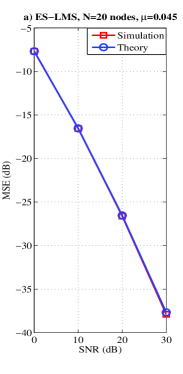
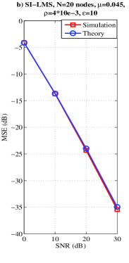
Figure 8: MSE performance against SNR for ES–LMS and SI–LMS

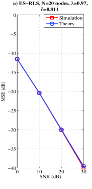
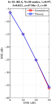
Figure 9: MSE performance against SNR for ES–RLS and SI–RLS

The tracking analysis of the proposed algorithms in a time–varying scenario is discussed as follows. Here, we verify that the results (77), (78), (79) and (80) of the subsection on the tracking analysis can provide a means of estimating the MSE. We consider the same model as in (81). In the next examples, we employ $N=20$ nodes in the network and the same parameters used to obtain the network MSE curves in a time–varying scenario. A comparison of the curves obtained by simulations and by the analytical formulas is shown in Figs. 10 and 11. From these curves, we can verify that the gap between the simulation and analysis results are within 0.02dB under different SNR values. The details of the parameters are shown on the top of each sub figure in Figs. 10 and 11.

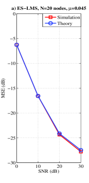
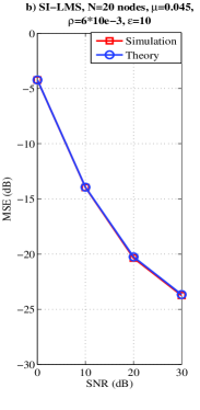
Figure 10: MSE performance against SNR for ES–LMS and SI–LMS in a time–-varying scenario

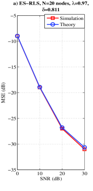
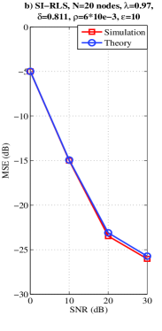
Figure 11: MSE performance against SNR for ES–RLS and SI–RLS in a time–-varying scenario

V-C Smart Grids

The proposed algorithms provide a cost–effective tool that could be used for distributed state estimation in smart grid applications. In order to test the proposed algorithms in a possible smart grid scenario, we consider the IEEE 14–bus system [52], where 14 is the number of substations. At every time instant $i$, each bus $k,k=1,2,\ldots,14,$ takes a scalar measurement $d_{k}(i)$ according to

$${d_{k}(i)}={X_{k}\big{(}{\boldsymbol{\omega}}_{0}(i)\big{)}+n_{k}(i)},~{}~{}~{}k=1,2,\ldots,14,$$ (82)

where $\boldsymbol{\omega}_{0}(i)$ is the state vector of the entire interconnected system, $X_{k}({\boldsymbol{\omega}}_{0}(i))$ is a nonlinear measurement function of bus $k$. The quantity ${n_{k}(i)}$ is the measurement error with mean equal to zero and which corresponds to bus $k$.

Initially, we focus on the linearized DC state estimation problem. The system is built with 1.0 per unit (p.u) voltage magnitudes at all buses and j1.0 p.u. branch impedance. Then, the state vector ${\boldsymbol{\omega}}_{0}(i)$ is taken as the voltage phase angle vector ${\boldsymbol{\omega}}_{0}$ for all buses. Therefore, the nonlinear measurement model for state estimation (82) is approximated by

$${d_{k}(i)}={\boldsymbol{x}_{k}^{H}(i)\boldsymbol{\omega}_{0}+n_{k}(i)},~{}~{}~{}k=1,2,\ldots,14,$$ (83)

where ${\boldsymbol{x}}_{k}(i)$ is the measurement Jacobian vector for bus $k$. Then, the aim of the distributed estimation algorithm is to compute an estimate of ${\boldsymbol{\omega}}_{0}$, which can minimize the cost function given by

$${J_{\boldsymbol{\omega}_{k}(i)}({\boldsymbol{\omega}_{k}(i)})}={\mathbb{E}|{d_{k}(i)}-{\boldsymbol{x}_{k}^{H}(i)}{\boldsymbol{\omega}_{k}(i)}|^{2}}.$$ (84)

We compare the proposed algorithms with the $\mathcal{M}$–$\mathcal{CSE}$ algorithm [4], the single link strategy [51], the standard diffusion RLS algorithm [50] and the standard diffusion LMS algorithm [2] in terms of MSE performance and the Phase Angle Gap. The MSE comparison is used to determine the accuracy of the algorithms, and the Phase Angle Gap is used to compare the rate of convergence. In our scenario, ’Phase Angle Gap’ refers to the phase angle difference between the actual parameter vector or target ${\boldsymbol{\omega}}_{0}$ and the estimate $\boldsymbol{\omega}_{k}(i)$ for all buses. We define the IEEE–14 bus system as in Fig. 12.

Figure 12: IEEE 14–bus system for simulation

All buses are corrupted by additive white Gaussian noise with equal variance $\sigma^{2}=0.001$. The step size for the standard diffusion LMS [2], the proposed ES–LMS and SI–LMS algorithms is 0.018. The parameter vector $\boldsymbol{\omega}_{0}$ is set to an all–one vector. For the diffusion RLS, ES–RLS and SI–RLS algorithms the forgetting factor $\lambda$ is set to 0.945 and $\delta$ is equal to 0.001. The sparsity parameters of the SI–LMS/RLS algorithms are set to $\rho=0.07$ and $\varepsilon=10$. The results are averaged over 100 independent runs. We simulate the proposed algorithms for smart grids under a static scenario.

Figure 13: MSE performance curves for smart grids.

From Fig. 13, it can be seen that ES–RLS has the best performance, and significantly outperforms the standard diffusion LMS [2] and the $\mathcal{M}$–$\mathcal{CSE}$ [4] algorithms. The ES–LMS is slightly worse than ES–RLS, which outperforms the remaining techniques. SI–RLS is worse than ES–LMS but is still better than SI–LMS, while SI–LMS remains better than the diffusion RLS, LMS, $\mathcal{M}$–$\mathcal{CSE}$ algorithms and the single link strategy.

Figure 14: Phase Angle Gap comparison for Bus 5.

In order to compare the convergence rate, we employ the ’Phase Angle Gap’ to describe the results. We choose bus 5 and the first 90 iterations as an example to illustrate our results. In Fig. 14, ES–RLS has the fastest convergence rate, while SI–LMS is the second fastest, followed by the standard diffusion RLS, ES–LMS, SI–LMS, and the standard diffusion LMS algorithms. The $\mathcal{M}$–$\mathcal{CSE}$ algorithm and the single link strategy have the worst performance. The estimates $\boldsymbol{\omega}_{k}(i)$ obtained by the proposed algorithms quickly reach the target ${\boldsymbol{\omega}}_{0}$, which means the Phase Angle Gap will converge to zero.

VI Conclusions

In this paper, we have proposed ES–LMS/RLS and SI–LMS/RLS algorithms for distributed estimation in applications such as wireless sensor networks and smart grids. We have compared the proposed algorithms with existing methods. We have also devised analytical expressions to predict their MSE steady–state performance and tracking behavior. Simulation experiments have been conducted to verify the analytical results and illustrate that the proposed algorithms significantly outperform the existing strategies, in both static and time–varying scenarios, in examples of wireless sensor networks and smart grids.

VII Acknowledgements

The authors wish to thank the anonymous reviewers, whose comments and suggestions have greatly improved the presentation of these results.

References

• [1] C. G. Lopes and A. H. Sayed, “Incremental adaptive strategies over distributed networks,” IEEE Trans. Signal Process., vol. 48, no. 8, pp. 223–229, Aug 2007.
• [2] ——, “Diffusion least-mean squares over adaptive networks: Formulation and performance analysis,” IEEE Trans. Signal Process., vol. 56, no. 7, pp. 3122–3136, July 2008.
• [3] Y. Chen, Y. Gu, and A. Hero, “Sparse LMS for system identification,” Proc. IEEE ICASSP, pp. 3125–3128, Taipei, Taiwan, May 2009.
• [4] L. Xie, D.-H. Choi, S. Kar, and H. V. Poor, “Fully distributed state estimation for wide-area monitoring systems,” IEEE Trans. Smart Grid, vol. 3, no. 3, pp. 1154–1169, September 2012.
• [5] D. Bertsekas, “A new class of incremental gradient methods for least squares problems,” SIAM J. Optim, vol. 7, no. 4, p. 913–926, 1997.
• [6] A. Nedic and D. Bertsekas, “Incremental subgradient methods for nondifferentiable optimization,” SIAM J. Optim, vol. 12, no. 1, p. 109–138, 2001.
• [7] M. G. Rabbat and R. D. Nowak, “Quantized incremental algorithms for distributed optimization,” IEEE J. Sel. Areas Commun, vol. 23, no. 4, p. 798–808, Apr 2005.
• [8] F. S. Cattivelli and A. H. Sayed, “Diffusion lms strategies for distributed estimation,” IEEE Trans. Signal Process., vol. 58, p. 1035–1048, March 2010.
• [9] P. D. Lorenzo, S. Barbarossa, and A. H. Sayed, “Sparse diffusion LMS for distributed adaptive estimation,” Proc. IEEE International Conference on Acoustics, Speech, and Signal Processing, pp. 3281–3284, Kyoto, Japan, March 2012.
• [10] S. Xu, R. C. de Lamare, and H. V. Poor, “Distributed compressed estimation based on compressive sensing,” IEEE Signal Processing Letters, vol. 22, no. 9, pp. 1311–1315, Sept 2015.
• [11] ——, “Adaptive link selection algorithms for distributed estimation,” EURASIP Journal on Advances in Signal Processing, vol. 2015, no. 1, pp. 1–22, October 2015.
• [12] C. Lopes and A. Sayed, “Diffusion adaptive networks with changing topologies,” in Proc. IEEE International Conference on Acoustics, Speech and Signal Processing, Las Vegas, 2008, pp. 3285–3288.
• [13] B. Fadlallah and J. Principe, “Diffusion least-mean squares over adaptive networks with dynamic topologies,” in Proc. IEEE International Joint Conference on Neural Networks, Dallas, TX, USA 2013.
• [14] T. Wimalajeewa and S. Jayaweera, “Distributed node selection for sequential estimation over noisy communication channels,” IEEE Trans. Wirel. Commun., vol. 9, no. 7, pp. 2290–2301, July 2010.
• [15] R. C. de Lamare and R. Sampaio-Neto, “Adaptive reduced-rank processing based on joint and iterative interpolation, decimation and filtering,” IEEE Trans. Signal Process., vol. 57, no. 7, pp. 2503–2514, July 2009.
• [16] R. C. de Lamare and P. S. R. Diniz, “Set-membership adaptive algorithms based on time-varying error bounds for CDMA interference suppression,” IEEE Trans. Vehi. Techn., vol. 58, no. 2, pp. 644–654, February 2009.
• [17] L. Guo and Y. F. Huang, “Frequency-domain set-membership filtering and its applications,” IEEE Trans. Signal Process., vol. 55, no. 4, pp. 1326–1338, April 2007.
• [18] A. Bertrand and M. Moonen, “Distributed adaptive node–specific signal estimation in fully connected sensor networks–part II: Simultaneous and asynchronous node updating,” IEEE Trans. Signal Process., vol. 58, no. 10, pp. 5292–5306, 2010.
• [19] S. Haykin, Adaptive Filter Theory, 4th ed.   Upper Saddle River, NJ, USA: Prentice Hall, 2002.
• [20] L. Li and J. A. Chambers, “Distributed adaptive estimation based on the APA algorithm over diffusion networks with changing topology,” in Proc. IEEE Statist. Signal Process. Workshop, pp. 757–760, Cardiff, Wales, September 2009.
• [21] X. Zhao and A. H. Sayed, “Performance limits for distributed estimation over lms adaptive networks,” IEEE Trans. Signal Process., vol. 60, no. 10, pp. 5107–5124, October 2012.
• [22] L. Xiao and S. Boyd, “Fast linear iterations for distributed averaging,” Syst. Control Lett., vol. 53, no. 1, pp. 65–78, September 2004.
• [23] R. Olfati-Saber and R. M. Murray, “Consensus problems in networks of agents with switching topology and time-delays,” IEEE Trans. Autom. Control., vol. 49, pp. 1520––1533, September 2004.
• [24] A. Jadbabaie, J. Lin, and A. S. Morse, “Coordination of groups of mobile autonomous agents using nearest neighbor rules,” IEEE Trans. Autom. Control, vol. 48, no. 6, pp. 988–1001, June 2003.
• [25] R. C. de Lamare and R. C. de Lamare, “Adaptive reduced-rank mmse filtering with interpolated fir filters and adaptive interpolators,” IEEE Signal Processing Letters, vol. 12, no. 3, March 2005.
• [26] R. Meng, R. C. de Lamare, and V. H. Nascimento, “Sparsity-aware affine projection adaptive algorithms for system identification,” in Proc. Sensor Signal Processing for Defence Conference, London, UK, 2011.
• [27] Z. Yang, R. de Lamare, and X. Li, “Sparsity-aware space-time adaptive processing algorithms with l1-norm regularisation for airborne radar,” Signal Processing, IET, vol. 6, no. 5, pp. 413–423, July 2012.
• [28] ——, “L1-regularized stap algorithms with a generalized sidelobe canceler architecture for airborne radar,” Signal Processing, IEEE Transactions on, vol. 60, no. 2, pp. 674–686, Feb 2012.
• [29] R. C. de Lamare and R. C. de Lamare, “Sparsity-aware adaptive algorithms based on alternating optimization and shrinkage,” IEEE Signal Processing Letters, vol. 21, no. 2, pp. 225–229, January 2014.
• [30] R. C. de Lamare and R. Sampaio-Neto, “Reduced–rank adaptive filtering based on joint iterative optimization of adaptive filters,” IEEE Signal Process. Lett., vol. 14, no. 12, pp. 980–983, December 2007.
• [31] ——, “Reduced-rank space–time adaptive interference suppression with joint iterative least squares algorithms for spread-spectrum systems,” IEEE Transactions Vehicular Technology, vol. 59, no. 3, pp. 1217–1228, March 2010.
• [32] ——, “Adaptive reduced-rank equalization algorithms based on alternating optimization design techniques for MIMO systems,” IEEE Transactions on Vehicular Technology, vol. 60, no. 6, pp. 2482–2494, July 2011.
• [33] ——, “Adaptive reduced-rank processing based on joint and iterative interpolation, decimation, and filtering,” IEEE Transactions on Signal Processing, vol. 57, no. 7, pp. 2503–2514, July 2009.
• [34] R. Fa, R. C. de Lamare, and L. Wang, “Reduced-rank stap schemes for airborne radar based on switched joint interpolation, decimation and filtering algorithm,” IEEE Transactions on Signal Processing, vol. 58, no. 8, pp. 4182–4194, August 2010.
• [35] S. Li, R. C. de Lamare, and R. Fa, “Reduced-rank linear interference suppression for ds-uwb systems based on switched approximations of adaptive basis functions,” IEEE Transactions on Vehicular Technology, vol. 60, no. 2, pp. 485–497, Feb 2011.
• [36] R. C. de Lamare, R. Sampaio-Neto, and M. Haardt, “Blind adaptive constrained constant-modulus reduced-rank interference suppression algorithms based on interpolation and switched decimation,” IEEE Transactions on Signal Processing, vol. 59, no. 2, pp. 681–695, Feb 2011.
• [37] M. L. Honig and J. S. Goldstein, “Adaptive reduced-rank interference suppression based on the multistage wiener filter,” IEEE Transactions on Communications, vol. 50, no. 6, June 2002.
• [38] R. C. de Lamare, M. Haardt, and R. Sampaio-Neto, “Blind adaptive constrained reduced-rank parameter estimation based on constant modulus design for cdma interference suppression,” IEEE Transactions on Signal Processing, vol. 56, no. 6, June 2008.
• [39] N. Song, R. C. de Lamare, M. Haardt, and M. Wolf, “Adaptive widely linear reduced-rank interference suppression based on the multi-stage wiener filter,” IEEE Transactions on Signal Processing, vol. 60, no. 8, August 2012.
• [40] H. Ruan and R. de Lamare, “Robust adaptive beamforming using a low-complexity shrinkage-based mismatch estimation algorithm,” Signal Processing Letters, IEEE, vol. 21, no. 1, pp. 60–64, Jan 2014.
• [41] Y. Chen, Y. Gu, and A. Hero, “Regularized least-mean-square algorithms,” Technical Report for AFOSR, December 2010.
• [42] S. Xu and R. C. de Lamare, “Distributed conjugate gradient strategies for distributed estimation over sensor networks,” in Proc. Sensor Signal Processing for Defence 2012, London, UK, 2012.
• [43] F. Cattivelli and A. H. Sayed, “Diffusion strategies for distributed kalman filtering and smoothing,” IEEE Trans. Autom. Control, vol. 55, no. 9, pp. 2069–2084, September 2010.
• [44] A. H. Sayed, Fundamentals of Adaptive Filtering.   Hoboken, NJ, USA: John Wiley&Sons, 2003.
• [45] T. Kailath, A. H. Sayed, and B. Hassibi, Linear Estimation.   Englewood Cliffs, NJ, USA: Prentice-Hall, 2000.
• [46] R. C. de Lamare and P. S. R. Diniz, “Blind adaptive interference suppression based on set-membership constrained constant-modulus algorithms with dynamic bounds,” IEEE Trans. Signal Process., vol. 61, no. 5, pp. 1288–1301, March 2013.
• [47] Y. Cai and R. C. de Lamare, “Low–complexity variable step-size mechanism for code-constrained constant modulus stochastic gradient algorithms applied to cdma interference suppression,” IEEE Trans. Signal Process., vol. 57, no. 1, pp. 313–323, January 2009.
• [48] B. Widrow and S. D. Stearns, Adaptive Signal Processing.   Englewood Cliffs, NJ, USA: Prentice-Hall, 1985.
• [49] E. Eweda, “Comparison of RLS, LMS, and sign algorithms for tracking randomly time-varying channels,” IEEE Trans. Signal Process., vol. 42, p. 2937–2944, November 1994.
• [50] F. Cattivelli, C. Lopes, and A. Sayed, “Diffusion recursive least-squares for distributed estimation over adaptive networks,” IEEE Trans. Signal Process., vol. 56, no. 5, pp. 1865–1877, May 2008.
• [51] X. Zhao and A. H. Sayed, “Single-link diffusion strategies over adaptive networks,” in Proc. IEEE International Conference on Acoustics, Speech and Signal Processing, pp. 3749–3752, Kyoto, Japan, March 2012.
• [52] A. Bose, “Smart transmission grid applications and their supporting infrastructure,” IEEE Trans. Smart Grid, vol. 1, no. 1, pp. 11–19, Jun 2010.