Spontaneous excitation of a static atom in a thermal bath in cosmic string spacetime

Abstract

We study the average rate of change of energy for a static atom immersed in a thermal bath of electromagnetic radiation in the cosmic string spacetime and separately calculate the contributions of thermal fluctuations and radiation reaction. We find that the transition rates are crucially dependent on the atom-string distance and polarization of the atom and they in general oscillate as the atom-string distance varies. Moreover, the atomic transition rates in the cosmic string spacetime can be larger or smaller than those in Minkowski spacetime contingent upon the atomic polarization and position. In particular, when located on the string, ground-state atoms can make a transition to excited states only if they are polarizable parallel to the string, whereas ground state atoms polarizable only perpendicular to the string are stable as if they were in a vacuum, even if they are immersed in a thermal bath. Our results suggest that the influence of a cosmic string is very similar to that of a reflecting boundary in Minkowski spacetime.

I INTRODUCTION

Spontaneous emission is one of the most important phenomena in the interaction of atoms with radiation, and it can be attributed to vacuum fluctuations Welton48 ; Compagno83 , or radiation reaction Ackerhalt73 , or a combination of them Milonni88 ; Milonni75 . So far, a lot of efforts have been made to resolve the ambiguity in the underlying mechanism regarding the radiative properties of atoms Milonni75 ; Vleck24 ; Dirac27 ; Ackerhalt73 ; Senitzky73 ; Milonni73 ; Ackerhalt74 ; Milonni752 . In this regard, Dalibard, Dupont-Roc and Cohen-Tannoudji (DDC) suggested a resolution which distinctively separates the contributions of vacuum fluctuations and radiation reaction by choosing a symmetric ordering between the operators of the dynamical variables of the atom and the field which ensures the Hermitianity of the Hamiltonians of vacuum fluctuations and radiation reaction Dalibard8284 . Later, the DDC formalism was generalized to investigate the radiative properties of atoms in different circumstances, such as a non-inertial atom in interaction with various quantum fields Audretsch94 ; Audretsch951 ; Passante98 ; Yu-na05 ; Yu-na061 ; Yu-na062 ; Yu-na07 ; Rizzuto07 ; Rizzuto09 ; Yu-na10 ; Rizzuto11 ; Yu-na12 , and an inertial atom immersed in a thermal bath Tomazelli03 ; Yu-th0912 ; Yu-th10 . In both cases, as the contribution of the fluctuations of the quantum field and that of the radiation reaction to the rate of change of the atomic energy no longer cancel completely, an atom in the ground state can make a spontaneous transition to excited states.

In recent years, investigations on the radiative properties of atoms have been extended to curved spacetime Iliadakis ; Yu-cur07 ; Yu-cur08 ; Yu-cur12 . It is interesting to note that these studies along with those for non-inertial atoms in flat spacetime have shed light on the nature of the Hawking radiation of black holes, the Gibbons-Hawking effect of de Sitter space as well as the Unruh effect related to uniformly accelerated observers as atoms can serve as a model of realistic particle detectors. In this paper, we plan to study the spontaneous excitation of static atoms in yet another typical curved spacetime, i.e., the spacetime of a cosmic string. In comparison to other spacetimes, the cosmic string spacetime is characterized by its structure with non-trivial topology, a planar deficit angle, to be specific. Although now much remains to be done to fully understand the behavior of strings, people are convinced that they may raise a number of issues in fundamental physics, for example, gravitational effects such as lensing of distant objects and conical bremsstrahlung Vilenkin81 ; Aliev89 ; Aliev93 . Interestingly, one can also use atoms to sense a cosmic string. In this respect, J. Audretsch, et al., studied the spontaneous emission and the Lamb shift of an atom in a toy model where the atom is assumed to be coupled to vacuum quantum scalar fields in the cosmic string spacetime and found that the spontaneous emission rate is modified by the presence of a cosmic string Audretsch952 . Recently, a number of authors have studied the Casimir effect and Casimir-Polder force in a more realistic situation where the atom interacts with electromagnetic vacuum fluctuations in the geometry of a straight cosmic string Saharian11 ; Saharian121 ; Saharian122 . In this paper, we plan to study the spontaneous excitation and emission of a static atom immersed in a thermal bath of electromagnetic radiation in the vicinity of a straight cosmic string, where the atom is coupled to quantum electromagnetic fields rather than scalar fields in Audretsch952 .

The paper is organized as follows. In section II, we introduce the quantization of electromagnetic fields in cosmic string space-time. In section III, we generalize the DDC formalism to study the average rate of change of the atomic energy in the cosmic string spacetime. In section IV, we concretely calculate the average rate of change of a static atom immersed in a thermal bath in the cosmic string spacetime and discuss how the conical deficit angle affects the rate of change of atomic energy. Finally in section V, we give some concluding remarks. Throughout the paper, we adopt the natural unit, $\hbar=c=1$, and let the Boltzmann constant $k_{B}=1$.

II Quantum electromagnetic field in the cosmic string space-time

The metric of a static, straight cosmic string lying along the $z$-direction in the cylindrical coordinate system is given by

$$ds^{2}=dt^{2}-d\rho^{2}-\rho^{2}d\theta^{2}-dz^{2}$$ (1)

where $0\leq\theta<\frac{2\pi}{\nu}$, $\nu=(1-4G\mu)^{-1}$ with $G$ and $\mu$ being the Newton’s constant and the mass per unit length of the string respectively. The Lagrangian density of the electromagnetic field can be written as

$$\mathcal{L}=\sqrt{-g}\biggl{[}-\frac{1}{4}F^{{}^{\mu\nu}}F_{{}_{\mu\nu}}-\frac{1}{2}(A^{\mu}_{\;;\mu})^{2}\biggr{]}\;.$$ (2)

The quantization of the field is to be carried out in the Feynman gauge

$$A^{\mu}_{\;;\mu}=0\;.$$ (3)

Inserting the above Lagrangian density into the Euler-Lagrangian equation, we obtain

$$F^{\mu\nu}_{\;\;\;\;;\nu}=0\;.$$ (4)

In terms of the vector potential of the electromagnetic field, the above equation becomes

$$\Box A_{\rho}-\frac{2}{\rho^{3}}\partial_{\theta}A_{\theta}-\frac{1}{\rho^{2}}A_{\rho}=0\;,$$ (5)

$$\Box A_{\theta}-\frac{2}{\rho}\partial_{\rho}A_{\theta}+\frac{2}{\rho}\partial_{\theta}A_{\rho}=0\;,$$ (6)

$$A_{z}=\Box A_{t}=0$$ (7)

with

$$\Box=\Delta-\partial_{tt}^{2},\quad\Delta=\frac{1}{\rho}\partial_{\rho}(\rho\partial_{\rho})+\frac{1}{\rho^{2}}\partial_{\theta\theta}^{2}+\partial_{zz}^{2}\;.$$ (8)

To solve Eqs. (5)-(7), we firstly decouple the field equations by introducing the spin-weighted components of the vector potential Aliev89 , i.e., define

$$A_{\xi}=\frac{1}{\sqrt{2}}(A_{\rho}+\frac{i\xi}{\rho}A_{\theta})\quad{\text{for}}\quad\xi=\pm 1,$$ (9)

$$A_{\xi}=A_{z},A_{t}\quad\quad\;{\text{for}}\quad\xi=3,0\;.$$ (10)

Then the decoupled field equations can be collectively written as

$$\Box_{\xi}A_{\xi}=0$$ (11)

with

$$\Box_{\xi}=\Delta_{\xi}-\partial_{tt}^{2}\;,$$ (12)

$$\Delta_{\xi}=\frac{1}{\rho}\partial_{\rho}(\rho\partial_{\rho})-\frac{1}{\rho^{2}}L_{3}^{2}+\partial_{tt}^{2}\;,$$ (13)

$$L_{3}=-i\partial_{\theta}+\xi\;.$$ (14)

The normal modes for the independent components, $A_{\xi}$, are

$$f_{\xi j}(x)=f_{\xi j}(\vec{x})e^{-i\omega t}$$ (15)

with

$$f_{\xi j}(\vec{x})=\frac{1}{2\pi}\sqrt{\frac{\nu}{2\omega}}J_{|\nu m+\xi|}(k_{\bot}\rho)e^{i(\nu m\theta+k_{3}z)}\;,$$ (16)

where the symbol $J$ denotes BesselJ function, the subscript $j=(k_{3},k_{\bot},m)$ and $\omega=\sqrt{k_{3}^{2}+k_{\bot}^{2}}$. The modes are normalized according to

$$\int d^{3}\bm{x}f_{\xi j}^{\ast}(x)(i\overleftrightarrow{\partial_{t}})f_{\xi j^{\prime}}(x)=\delta_{j,j^{\prime}}=\delta_{m,m^{\prime}}\delta(k_{3}-k_{3}^{\prime})\frac{\delta(k_{\bot}-k_{\bot}^{\prime})}{\sqrt{k_{\bot}k_{\bot}^{\prime}}}.$$ (17)

In order to quantize the electromagnetic field, we define the canonically conjugate field $\Pi^{\mu}$ corresponding to $A_{\mu}$ as

$$\Pi_{\mu}=\frac{1}{\sqrt{-g}}\frac{\partial{\mathcal{L^{\prime}}}}{\partial{A^{\mu}_{\;\;;0}}}=-A_{\mu}^{\;\;;0}$$ (18)

in which $\mathcal{L}^{\prime}$ describes the dynamics of the electromagnetic field and it is obtained by discarding a four-divergence term in $\mathcal{L}$ which has no influence on the field equations. We impose the following equal-time commutation relations for the field operator $A^{\mu}$ and $\Pi^{\mu}$

$$[A_{\mu}(t,\vec{x}),A_{\nu}(t,\vec{x})]=[\Pi_{\mu}(t,\vec{x}),\Pi_{\nu}(t,\vec{x})]=0,\\$$ (19)

$$[A_{\mu}(t,\vec{x}),\Pi^{\nu}(t,\vec{x}^{\prime})]=i\delta_{\mu}^{\nu}\delta^{3}(\vec{x}-\vec{x}^{\prime})\;.$$ (20)

Now we expand the field operator in terms of the complete set of normal modes (see Eq. (15)),

$$A_{\xi}(t,\vec{x})=\int d\mu_{j}\;[\;c_{\xi j}(t)f_{\xi j}(\vec{x})+c_{-\xi j}^{{\dagger}}(t)f_{-\xi j}^{\ast}(\vec{x})]$$ (21)

in which

$$\int d\mu_{j}=\sum_{m=-\infty}^{\infty}\int_{-\infty}^{\infty}dk_{3}\int_{0}^{\infty}dk_{\perp}k_{\perp}\;,$$ (22)

and $c_{\xi j}(t)=c_{\xi j}(0)e^{-i\omega t}$ and $c^{{\dagger}}_{-\xi j}=c^{{\dagger}}_{-\xi j}(0)e^{i\omega t}$ are respectively the annihilation and creation operators for a photon with quantum numbers $(k_{3},k_{\perp},m)$ at time $t$. One can show that

$$c_{\xi j}(0) = i\int d^{3}\vec{x}f^{\ast}_{\xi j}(t,x)\overleftrightarrow{\partial_{t}}A_{\xi}(t,x)\;,$$ (23)

$$c^{{\dagger}}_{\xi j}(0) = -i\int d^{3}\vec{x}f_{\xi j}(t,x)\overleftrightarrow{\partial_{t}}A_{\xi}(t,x)\;.$$ (24)

Now by using the relations Eqs. (9), (10), (19), (20), the commutation relations of the annihilation and creation operators are found to be

$$[c_{\xi j}(t),c_{\xi j^{\prime}}^{{\dagger}}(t)]=\delta_{j,j^{\prime}}\quad\;for\quad\xi=\pm 1,3,$$ (25)

$$[c_{0j}(t),c_{0j^{\prime}}^{{\dagger}}(t)]=-\delta_{j,j^{\prime}}\;\;for\quad\xi=0.$$ (26)

Here let us point out that a minus sign in the commutation relations for $\xi=0$ in Eq. (26), which is missing in Ref. Skarzhinsky94 , has been added.

Finally by calculating the $T_{00}$ component of the stress tensor of the quantum electromagnetic field, we obtain the Hamiltonian operator of the field

$$H_{F}=\int d\mu_{j}\;\omega_{j}(c_{+j}^{{\dagger}}c_{+j}+c_{-j}^{{\dagger}}c_{-j}+c_{3j}^{{\dagger}}c_{3j}-c_{0j}^{{\dagger}}c_{0j})\;.$$ (27)

III The generalized DDC formalism

We consider a multi-level atom in interaction with the quantum electromagnetic field in a thermal bath in the cosmic string space-time. The Hamiltonian that governs the evolution of the atom with respect to the proper time, $\tau$, is given by

$$H_{A}(\tau)=\sum_{n}\omega_{n}\sigma_{nn}(\tau)\;,$$ (28)

in which $\sigma_{nn}=|n\rangle\langle n|$ and $|n\rangle$ denotes a complete set of atomic stationary state with energy $\omega_{n}$. The Hamiltonian of the quantum electromagnetic field in the proper time, $\tau$, is

$$H_{F}(\tau)=\int d\mu_{j}\;\omega_{j}(c_{+j}^{{\dagger}}c_{+j}+c_{-j}^{{\dagger}}c_{-j}+c_{3j}^{{\dagger}}c_{3j}-c_{0j}^{{\dagger}}c_{0j})\frac{dt}{d\tau}\;.$$ (29)

We assume that the atom interacts with the quantum electromagnetic field in the multipolar coupling scheme Passante98 , so the interaction Hamitonian can be written as

$$H_{I}(\tau)=-e\textbf{r}(\tau)\cdot\textbf{E}(x(\tau))=-e\sum_{mn}\textbf{r}_{mn}\cdot\textbf{E}(x(\tau))\sigma_{mn}(\tau)$$ (30)

where $e$ is the electron electric charge, $e\textbf{r}$ is the atomic dipole moment, and $x(\tau)\leftrightarrow(t(\tau),\vec{x}(\tau))$ is the space-time coordinate of the atom in the cosmic string spacetime. The Hamiltonain that determines the time evolution of the system (atom+field) is composed by the above three parts

$$H(\tau)=H_{A}(\tau)+H_{F}(\tau)+H_{I}(\tau).$$ (31)

Starting from the above Hamiltonian, we can write out the Heisenberg equations for the dynamical variables of the atom and the field. In the formal solutions, we can separate each solution of either the variable of the atom or the field into the “free” part which exists even in the vacuum, and the “source” part which is induced by the interaction between the atom and the field,

$$\sigma_{mn}(\tau) = \sigma_{mn}^{f}(\tau)+\sigma_{mn}^{s}(\tau)\;,$$ (32)

$$c_{\xi j}(t(\tau)) = c_{\xi j}^{f}(t(\tau))+c_{\xi j}^{s}(t(\tau))\;,$$ (33)

where

$$\left\{\begin{array}[]{ll}c_{\xi j}^{f}(t(\tau))=c_{\xi j}(t(\tau_{0}))e^{-i\omega_{j}[t(\tau)-t(\tau_{0})]}\;,\\ c_{\xi j}^{s}(t(\tau))=-ie\int_{\tau_{0}}^{\tau}d\tau^{\prime}\;[\textbf{r}(\tau^{\prime})\cdot\textbf{E}(x(\tau^{\prime})),c_{\xi j}^{f}(t(\tau))]\;,\end{array}\right.$$ (36)

and

$$\left\{\begin{array}[]{ll}\sigma_{mn}^{f}(\tau)=\sigma_{mn}^{f}(\tau_{0})e^{i\omega_{mn}(\tau-\tau_{0})}\;,\\ \sigma_{mn}^{s}(\tau)=-ie\int_{\tau_{0}}^{\tau}d\tau^{\prime}\;[\textbf{r}(\tau^{\prime})\cdot\textbf{E}(x(\tau^{\prime})),\sigma_{mn}^{f}(\tau)]\;.\end{array}\right.$$ (39)

Consequently, the free part and source part of the vector potential operator can be expressed as

$$A^{f}_{\xi}(t,\vec{x}) = \int d\mu_{j}\;[\;c^{f}_{\xi j}(t)f_{\xi j}(\vec{x})+{c^{f{\dagger}}_{-\xi j}}(t)f_{-\xi j}^{\ast}(\vec{x})]\;,$$ (40)

$$A_{\xi}^{s}(t,\vec{x}) = -ie\int_{\tau_{0}}^{\tau}d\tau^{\prime}\;[\textbf{r}^{f}(\tau^{\prime})\cdot\textbf{E}^{f}(x(\tau^{\prime})),A_{\xi}^{f}(x(\tau))]\;.$$ (41)

Notice that in the source parts of the above solutions, all operators on the right-hand side have been replaced by their free parts, which are correct to the first order in $e$.

Taking the observable to be the energy of the atom, we obtain

$$\frac{dH_{A}(\tau)}{d\tau}=-ie[\textbf{r}(\tau)\cdot\textbf{E}(x(\tau)),H_{A}(\tau)]\;.$$ (42)

Now following DDC Dalibard8284 , we separate the field operator into the free part and the source part, $\textbf{E}(x(\tau))=\textbf{E}^{f}(x(\tau))+\textbf{E}^{s}(x(\tau))$, and choose a symmetric ordering between the operators of the variables of the atom and the field. Then we can identify the contributions of the free part and the source part, i.e., the contributions of thermal fluctuations and radiation reaction,

$$\frac{dH_{A}(\tau)}{d\tau}=\biggl{(}\frac{dH_{A}(\tau)}{d\tau}\biggr{)}_{tf}+\biggl{(}\frac{dH_{A}(\tau)}{d\tau}\biggr{)}_{rr}$$ (43)

with

$$\biggl{(}\frac{dH_{A}(\tau)}{d\tau}\biggr{)}_{tf} = -\frac{ie}{2}(\textbf{E}^{f}(x(\tau))\cdot[\textbf{r}^{f}(\tau),H_{A}(\tau)]+[\textbf{r}^{f}(\tau),H_{A}(\tau)]\cdot\textbf{E}^{f}(x(\tau)))\;,$$ (44)

$$\biggl{(}\frac{dH_{A}(\tau)}{d\tau}\biggr{)}_{rr} = -\frac{ie}{2}(\textbf{E}^{s}(x(\tau))\cdot[\textbf{r}^{f}(\tau),H_{A}(\tau)]+[\textbf{r}^{f}(\tau),H_{A}(\tau)]\cdot\textbf{E}^{s}(x(\tau)))\;.$$ (45)

Averaging the above two equations over the state of the field, $|\beta\rangle$, and the atomic state, $|a\rangle$, we obtain, after some simplifications, the contributions of thermal fluctuations and radiation reaction to the average rate of change of the atomic energy,

$$\biggl{\langle}\frac{dH_{A}(\tau)}{d\tau}\biggr{\rangle}_{tf} = 2ie^{2}\int_{\tau_{0}}^{\tau}d\tau^{\prime}C_{ij}^{F\beta}(x(\tau),x(\tau^{\prime}))\frac{d}{d\tau}\chi^{ijA}_{b}(\tau,\tau^{\prime})\;,$$ (46)

$$\biggl{\langle}\frac{dH_{A}(\tau)}{d\tau}\biggr{\rangle}_{rr} = 2ie^{2}\int_{\tau_{0}}^{\tau}d\tau^{\prime}\chi_{ij}^{F\beta}(x(\tau),x(\tau^{\prime}))\frac{d}{d\tau}C^{ijA}_{b}(\tau,\tau^{\prime})\;,$$ (47)

where $C_{ij}^{F\beta}(x(\tau),x(\tau^{\prime}))$ and $\chi_{ij}^{F\beta}(x(\tau),x(\tau^{\prime}))$ are respectively the symmetric correlation function and the linear susceptibility function of the quantum electromagnetic field defined as

$$C_{ij}^{F\beta}(x(\tau),x(\tau^{\prime})) = \frac{1}{2}\langle\beta|\{E_{i}^{f}(x(\tau)),E_{j}^{f}(x(\tau^{\prime}))\}|\beta\rangle\;,$$ (48)

$$\chi_{ij}^{F\beta}(x(\tau),x(\tau^{\prime})) = \frac{1}{2}\langle\beta|[E_{i}^{f}(x(\tau)),E_{j}^{f}(x(\tau^{\prime}))]|\beta\rangle\;,$$ (49)

and $C^{ijA}_{b}(\tau,\tau^{\prime})$ and $\chi^{ijA}_{b}(\tau,\tau^{\prime})$ are the two statistical functions of the atom in state $|b\rangle$ which are defined as follows

$$C^{ijA}_{b}(\tau,\tau^{\prime}) = \frac{1}{2}\sum_{d}[\langle b|r^{i}(0)|d\rangle\langle d|r^{j}(0)|b\rangle e^{i\omega_{bd}(\tau-\tau^{\prime})}+\langle b|r^{j}(0)|d\rangle\langle d|r^{i}(0)|b\rangle e^{-i\omega_{bd}(\tau-\tau^{\prime})}]\;,$$

$$\chi^{ijA}_{b}(\tau,\tau^{\prime}) = \frac{1}{2}\sum_{d}[\langle b|r^{i}(0)|d\rangle\langle d|r^{j}(0)|b\rangle e^{i\omega_{bd}(\tau-\tau^{\prime})}-\langle b|r^{j}(0)|d\rangle\langle d|r^{i}(0)|b\rangle e^{-i\omega_{bd}(\tau-\tau^{\prime})}]\;$$

where $\omega_{bd}=\omega_{b}-\omega_{d}$ and the sum extends over a complete set of atomic states.

IV Rate of change of the energy of a static atom

Assume that an atom is placed static in a thermal bath with temperature $T$ in the cosmic string spacetime. In the cylindrical coordinates we use, the position of the atom is denoted by $x(\tau)=(t(\tau),\rho,\theta,\phi)$ where $\rho,\theta,\phi$ are constants. As we have shown in the preceding Section, in order to calculate the average rate of change of the atomic energy, details on the two statistical functions of the field are indispensable. Combine Eqs. (9), (10) with Eq. (21), and then we get

$$A_{\rho}(t,\vec{x}) = \frac{1}{\sqrt{2}}\int d\mu_{j}[(c_{+j}f_{+j}+c_{-j}f_{-j})+(c_{+j}^{{\dagger}}f_{+j}^{\ast}+c_{-j}^{{\dagger}}f_{-j}^{\ast})]\;,$$ (52)

$$A_{\theta}(t,\vec{x}) = -\frac{i\rho}{\sqrt{2}}\int d\mu_{j}[(c_{+j}f_{+j}-c_{-j}f_{-j})-(c_{+j}^{{\dagger}}f_{+j}^{\ast}-c_{-j}^{{\dagger}}f_{-j}^{\ast})]\;,$$ (53)

$$A_{z,t}(t,\vec{x}) = \int d\mu_{j}[c_{3j,0j}f_{0j}+c_{3j,0j}^{{\dagger}}f_{0j}^{\ast}]\;,$$ (54)

where we have used the abbreviations $c_{+j}(t)\leftrightarrow c_{+j}$ and $f_{\xi j}(\vec{x})\leftrightarrow f_{\xi j}$. Making use of the relation $E_{i}=A_{0;i}-A_{i;0}$ leads to

$$\langle\beta|E_{i}(x)E_{j}(x^{\prime})|\beta\rangle=\partial_{0}\partial_{0}^{\prime}\langle\beta|A_{i}(x)A_{j}(x^{\prime})|\beta\rangle+\partial_{i}\partial_{j}^{\prime}\langle\beta|A_{0}(x)A_{0}(x^{\prime})|\beta\rangle\;.$$ (55)

The average value of an arbitrary operator, $G$, over the thermal state $|\beta\rangle$, can be obtained by using the following formula

$$\langle\beta|G|\beta\rangle=\frac{tr[\rho G]}{tr[\rho]}\;,$$ (56)

where $\rho=e^{-\beta H_{F}}$ with $\beta=T^{-1}$ being the density matrix. Combining Eqs. (52)-(56) with Eq. (48), the non-zero components of the correlation functions of the field are found to be

$$C_{11}^{F\beta}(x(\tau),x(\tau^{\prime})) = \frac{\nu}{8\pi^{2}}\int d\mu_{j}\coth(\omega/T)\cos(\mathcal{}\omega(t-t^{\prime}))$$ (57)

$$\quad\times\biggl{[}\frac{\omega}{2}(J_{|\nu m+1|}^{2}(k_{\perp}\rho)+J_{|\nu m-1|}^{2}(k_{\perp}\rho))-\frac{1}{\omega}\biggl{(}\frac{dJ_{|\nu m|}(k_{\perp}\rho)}{d\rho}\biggr{)}^{2}\biggr{]}\;,$$

$$C_{22}^{F\beta}(x(\tau),x(\tau^{\prime})) = \frac{\nu\rho^{2}}{8\pi^{2}}\int d\mu_{j}\coth(\omega/T)\cos(\mathcal{}\omega(t-t^{\prime}))$$ (58)

$$\quad\times\biggl{[}\frac{\omega}{2}(J_{|\nu m+1|}^{2}(k_{\perp}\rho)+J_{|\nu m-1|}^{2}(k_{\perp}\rho))-\frac{1}{\omega}\frac{\nu^{2}m^{2}}{\rho^{2}}J^{2}_{|\nu m|}(k_{\perp}\rho)\biggr{]}\;,$$

$$C_{33}^{F\beta}(x(\tau),x(\tau^{\prime})) = \frac{\nu}{8\pi^{2}}\int d\mu_{j}\;\frac{k_{\perp}^{2}}{\omega}\coth(\omega/T)J_{|\nu m|}^{2}(k_{\perp}\rho)\cos(\mathcal{}\omega(t-t^{\prime}))\;.$$ (59)

Similarly, a combination of Eqs. (52)-(56) with Eq. (49) gives the non-zero components of the susceptibility functions of the field

$$\chi_{11}^{F\beta}(x(\tau),x(\tau^{\prime})) = -\frac{i\nu}{8\pi^{2}}\int d\mu_{j}\sin(\mathcal{}\omega(t-t^{\prime}))$$ (60)

$$\quad\times\biggl{[}\frac{\omega}{2}(J_{|\nu m+1|}^{2}(k_{\perp}\rho)+J_{|\nu m-1|}^{2}(k_{\perp}\rho))-\frac{1}{\omega}\biggl{(}\frac{dJ_{|\nu m|}(k_{\perp}\rho)}{d\rho}\biggr{)}^{2}\biggr{]}\;,$$

$$\chi_{22}^{F\beta}(x(\tau),x(\tau^{\prime})) = -\frac{i\nu\rho^{2}}{8\pi^{2}}\int d\mu_{j}\sin(\mathcal{}\omega(t-t^{\prime}))$$ (61)

$$\quad\times\biggl{[}\frac{\omega}{2}(J_{|\nu m+1|}^{2}(k_{\perp}\rho)+J_{|\nu m-1|}^{2}(k_{\perp}\rho))-\frac{1}{\omega}\frac{\nu^{2}m^{2}}{\rho^{2}}J^{2}_{|\nu m|}(k_{\perp}\rho)\biggr{]}\;,$$

$$\chi_{33}^{F\beta}(x(\tau),x(\tau^{\prime})) = -\frac{i\nu}{8\pi^{2}}\int d\mu_{j}\frac{k_{\perp}^{2}}{\omega}J_{|\nu m|}^{2}(k_{\perp}\rho)\sin(\mathcal{}\omega(t-t^{\prime}))\;.$$ (62)

Insert the correlation functions of the field (Eqs. (57)-(59)) and the antisymmetric statistical functions of the atom (Eq. (III)) into Eq. (46), assume that $\tau-\tau_{0}\rightarrow\infty$, make the coordinate transformation, $k_{\perp}=\omega\sin\alpha,k_{3}=\omega\cos\alpha$ in which $\alpha\in[0,\pi]$, $\omega\in[0,\infty)$, and then we obtain, after some lengthy simplifications, the contributions of thermal fluctuations to the average rate of change of the atomic energy

$$\biggr{\langle}\frac{dH_{A}(\tau)}{d\tau}\biggr{\rangle}_{tf} = -\frac{e^{2}}{3\pi}\sum_{\omega_{bd}>0}\omega^{4}_{bd}|\langle b|\mathrm{r}_{i}(0)|d\rangle|^{2}f_{i}(\omega_{bd},\rho,\nu)\biggl{(}\frac{1}{2}+\frac{1}{e^{\omega_{bd}/T}-1}\biggr{)}$$ (63)

$$+\frac{e^{2}}{3\pi}\sum_{\omega_{bd}<0}\omega^{4}_{bd}|\langle b|\mathrm{r}_{i}(0)|d\rangle|^{2}f_{i}(|\omega_{bd}|,\rho,\nu)\biggl{(}\frac{1}{2}+\frac{1}{e^{|\omega_{bd}|/T}-1}\biggr{)}\;,$$

where we have defined

$$f_{1}(\omega,\rho,\nu) = \frac{3\nu}{4}\sum_{m}\int_{0}^{1}dt\frac{t}{\sqrt{1-t^{2}}}[(2-t^{2})J^{2}_{|\nu m+1|}(\omega\rho t)+t^{2}J_{|\nu m|+1}(\omega\rho t)J_{|\nu m|-1}(\omega\rho t)]\;,$$

$$f_{2}(\omega,\rho,\nu) = \frac{3\nu}{4}\sum_{m}\int_{0}^{1}dt\frac{t}{\sqrt{1-t^{2}}}[(2-t^{2})J^{2}_{|\nu m+1|}(\omega\rho t)-t^{2}J_{|\nu m|+1}(\omega\rho t)J_{|\nu m|-1}(\omega\rho t)]\;,$$

$$f_{3}(\omega,\rho,\nu) = \frac{3\nu}{2}\sum_{m}\int_{0}^{1}dt\frac{t^{3}}{\sqrt{1-t^{2}}}J^{2}_{|\nu m|}(\omega\rho t)\;.$$ (66)

In obtaining the above results, we have used the following properties of the BesselJ functions:

$$\sum_{m}J^{2}_{|\nu m+1|}(x)=\sum_{m}J^{2}_{|\nu m-1|}(x)\;,$$ (67)

$$\sum_{m}J^{2}_{|\nu m|+1}(x)+\sum_{m}J^{2}_{|\nu m|-1}(x)=2\sum_{m}J^{2}_{|\nu m+1|}(x)\;,(\nu\geq 1)$$ (68)

It is easy to show that functions $f_{i}(\omega,\rho,\nu)$ are always positive. For an atom in the excited state, only the first term in Eq. (63), which is negative, contributes, while for an atom in the ground state, only the second term in Eq. (63), which is positive, contributes, i.e., the thermal fluctuations always de-excite an atom in the excited state and excite it in the ground state. This is similar to what happens to an atom in Minkowski spacetime with no boundaries Audretsch94 . However, there are also some sharp differences between the two cases. Obviously, as can be seen from Eq. (63), in the cosmic string spacetime, the contribution of thermal fluctuations depends on the polarization and the position of the atom, which is similar to a static atom in the Minkowski spacetime with boundaries Yu-na061 ; Yu-na062 ; Yu-th0912 , while in a free Minkowski spactime with no boundaries, the contribution of thermal fluctuations does not depend on the polarization and position of the atom Audretsch94 .

Similarly, plug the correlation functions of the field (Eqs. (60)-(62)) and the symmetric statistical function (Eq. (LABEL:cA)) of the atom into Eq. (47), do some simplifications, and then we obtain the contribution of radiation reaction to the average rate of change of the atomic energy,

$$\biggr{\langle}\frac{dH_{A}(\tau)}{d\tau}\biggr{\rangle}_{rr} = -\frac{e^{2}}{6\pi}\sum_{\omega_{bd}>0}\omega^{4}_{bd}|\langle b|\mathrm{r}_{i}(0)|d\rangle|^{2}f_{i}(\omega_{bd},\rho,\nu)$$ (69)

$$-\frac{e^{2}}{6\pi}\sum_{\omega_{bd}<0}\omega^{4}_{bd}|\langle b|\mathrm{r}_{i}(0)|d\rangle|^{2}f_{i}(|\omega_{bd}|,\rho,\nu)\;.$$

For both the ground and the excited-state atoms, the contribution of the radiation reaction is always negative. So just as in a free Minkowski spacetime Audretsch94 , radiation reaction always diminishes the atomic energy. Comparing this result with the contribution of thermal fluctuations, Eq. (63), we find that both contributions of thermal fluctuations and radiation reaction depend on the polarization and position of the atom.

Adding up Eqs. (63) and (69), we arrive at the total average rate of change of the atomic energy,

$$\biggr{\langle}\frac{dH_{A}(\tau)}{d\tau}\biggr{\rangle}_{tot} = -\frac{e^{2}}{3\pi}\sum_{\omega_{bd}>0}\omega^{4}_{bd}|\langle b|\mathrm{r}_{i}(0)|d\rangle|^{2}f_{i}(\omega_{bd},\rho,\nu)\biggl{(}1+\frac{1}{e^{\omega_{bd}/T}-1}\biggr{)}$$ (70)

$$+\frac{e^{2}}{3\pi}\sum_{\omega_{bd}<0}\omega^{4}_{bd}|\langle b|\mathrm{r}_{i}(0)|d\rangle|^{2}f_{i}(|\omega_{bd}|,\rho,\nu)\frac{1}{e^{|\omega_{bd}|/T}-1}\;.$$

For an atom in the excited state, the first term, which is negative, contributes. It describes the spontaneous emission rate of the excited atom immersed in a thermal bath in the cosmic string spacetime. For an atom in the ground state, the second term contributes and it is always positive. It describes the spontaneous excitation rate of the atom. This is clearly distinct from the transition rate of an inertial atom in the ground state in vacuum,

$$\biggr{\langle}\frac{dH_{A}(\tau)}{d\tau}\biggr{\rangle}_{tot}^{vac}=-\frac{e^{2}}{3\pi}\sum_{\omega_{bd}>0}\omega^{4}_{bd}|\langle b|\mathrm{r}_{i}(0)|d\rangle|^{2}f_{i}(\omega_{bd},\rho,\nu)\;,$$ (71)

which is obtained by taking $T=0$ in Eq. (70). Obviously, the rate of change of the ground state atom reduces to zero as a result of the complete cancelation of the contributions of vacuum fluctuations and radiation reaction, i.e., for a ground-state atom placed in a vacuum in the cosmic string spacetime, no spontaneous excitation occurs.

Generally, analytical expressions for the functions $f_{i}(\omega,\rho,\nu)$ are not easy to find, but in some special cases, approximate analytical results are obtainable. We will examine these cases in the following.

IV.1 The case for $\nu=1$.

The case when $\nu=1$ corresponds to a flat spacetime without cosmic strings. As a result of the following properties of the BesselJ function,

$$\sum_{m}J^{2}_{|m|}(x)=1\;,\quad\quad\sum_{m}J_{|m|+1}(x)J_{|m|-1}(x)=0\;,$$ (72)

$f_{i}(\omega,\rho,\nu)=1$ ($i=1,2,3$). So, the contributions of thermal fluctuations and radiation reaction to the average rate of change of the atomic energy reduce to

$$\biggr{\langle}\frac{dH_{A}(\tau)}{d\tau}\biggr{\rangle}_{tf} = -\frac{e^{2}}{3\pi}\sum_{\omega_{bd}>0}\omega^{4}_{bd}|\langle b|\textbf{r}(0)|d\rangle|^{2}\biggl{(}\frac{1}{2}+\frac{1}{e^{\omega_{bd}/T}-1}\biggr{)}$$ (73)

$$+\frac{e^{2}}{3\pi}\sum_{\omega_{bd}<0}\omega^{4}_{bd}|\langle b|\textbf{r}(0)|d\rangle|^{2}\biggl{(}\frac{1}{2}+\frac{1}{e^{|\omega_{bd}|/T}-1}\biggr{)}\;,$$

$$\biggr{\langle}\frac{dH_{A}(\tau)}{d\tau}\biggr{\rangle}_{rr} = -\frac{e^{2}}{3\pi}\sum_{\omega_{bd}>0}\omega^{4}_{bd}|\langle b|\textbf{r}(0)|d\rangle|^{2}\biggl{(}\frac{1}{2}+\frac{1}{e^{\omega_{bd}/T}-1}\biggr{)}$$ (74)

$$-\frac{e^{2}}{3\pi}\sum_{\omega_{bd}<0}\omega^{4}_{bd}|\langle b|\textbf{r}(0)|d\rangle|^{2}\biggl{(}\frac{1}{2}+\frac{1}{e^{|\omega_{bd}|/T}-1}\biggr{)}\;,$$

where we have used the abbreviation,

$$|\langle b|\textbf{r}(0)|d\rangle|^{2}=\sum_{i}|\langle b|\mathrm{r}_{i}(0)|d\rangle|^{2}\;.$$ (75)

Thus the total rate of change of the atomic energy becomes

$$\biggr{\langle}\frac{dH_{A}(\tau)}{d\tau}\biggr{\rangle}_{tot} = -\frac{e^{2}}{3\pi}\sum_{\omega_{bd}>0}\omega^{4}_{bd}|\langle b|\textbf{r}(0)|d\rangle|^{2}\biggl{(}1+\frac{1}{e^{\omega_{bd}/T}-1}\biggr{)}$$ (76)

$$+\frac{e^{2}}{3\pi}\sum_{\omega_{bd}<0}\omega^{4}_{bd}|\langle b|\textbf{r}(0)|d\rangle|^{2}\frac{1}{e^{|\omega_{bd}|/T}-1}$$

which is just the average rate of change of an inertial atom placed in a thermal bath with temperature $T$ in a free Minkowski spacetime, i.e., when $\nu=1$, the result in Minkowski spacetime is recovered as expected.

IV.2 The case for $\nu>1$.

Let us note that when $\omega\rho\ll 1$, one has

$$f_{1}(\omega,\rho,\nu)\approx f_{2}(\omega,\rho,\nu)\approx\frac{3\nu^{2}(\nu+1)}{\Gamma[2\nu+2]}(\omega\rho)^{2(\nu-1)}\equiv g(\omega\rho,\nu)\;,\quad f_{3}(\omega,\rho,\nu)\approx\nu\;.$$ (77)

So, when $\rho\ll\omega_{max}^{-1}$ where $\omega_{max}$ denotes the largest energy gap between two levels of the atom, the contribution of thermal fluctuations reduces to

$$\biggr{\langle}\frac{dH_{A}(\tau)}{d\tau}\biggr{\rangle}_{tf} \approx -\frac{e^{2}}{3\pi}\sum_{\omega_{bd}>0}\omega^{4}_{bd}[|\langle b|\mathrm{r}_{\perp}(0)|d\rangle|^{2}g(\omega_{bd}\rho,\nu)+|\langle b|\mathrm{r}_{z}(0)|d\rangle|^{2}\nu]\biggl{(}\frac{1}{2}+\frac{1}{e^{\omega_{bd}/T}-1}\biggr{)}$$

$$+\frac{e^{2}}{3\pi}\sum_{\omega_{bd}<0}\omega_{bd}^{4}[|\langle b|\mathrm{r}_{\perp}(0)|d\rangle|^{2}g(|\omega_{bd}|\rho,\nu)+|\langle b|\mathrm{r}_{z}(0)|d\rangle|^{2}\nu]\biggl{(}\frac{1}{2}+\frac{1}{e^{|\omega_{bd}|/T}-1}\biggr{)}$$

where we have defined

$$|\langle b|\mathrm{r}_{\perp}(0)|d\rangle|^{2}=\sum_{i=1}^{2}|\langle b|\mathrm{r}_{i}(0)|d\rangle|^{2}\;,$$ (79)

and we call this region ($\rho\ll\omega_{max}^{-1}$) the near zone. The contribution of radiation reaction becomes

$$\biggr{\langle}\frac{dH_{A}(\tau)}{d\tau}\biggr{\rangle}_{rr} \approx -\frac{e^{2}}{6\pi}\sum_{\omega_{bd}>0}\omega^{4}_{bd}[|\langle b|\mathrm{r}_{\perp}(0)|d\rangle|^{2}g(\omega_{bd}\rho,\nu)+|\langle b|\mathrm{r}_{z}(0)|d\rangle|^{2}\nu]$$ (80)

$$+\frac{e^{2}}{6\pi}\sum_{\omega_{bd}<0}\omega_{bd}^{4}[|\langle b|\mathrm{r}_{\perp}(0)|d\rangle|^{2}g(|\omega_{bd}|\rho,\nu)+|\langle b|\mathrm{r}_{z}(0)|d\rangle|^{2}\nu]\;.$$

As a result, the total average rate of change of the atomic energy can be written as

$$\biggr{\langle}\frac{dH_{A}(\tau)}{d\tau}\biggr{\rangle}_{tot} \approx -\frac{e^{2}}{3\pi}\sum_{\omega_{bd}>0}\omega^{4}_{bd}[|\langle b|\mathrm{r}_{\perp}(0)|d\rangle|^{2}g(\omega_{bd}\rho,\nu)+|\langle b|\mathrm{r}_{z}(0)|d\rangle|^{2}\nu]\biggl{(}1+\frac{1}{e^{\omega_{bd}/T}-1}\biggr{)}$$ (81)

$$+\frac{e^{2}}{3\pi}\sum_{\omega_{bd}<0}\omega_{bd}^{4}[|\langle b|\mathrm{r}_{\perp}(0)|d\rangle|^{2}g(|\omega_{bd}|\rho,\nu)+|\langle b|\mathrm{r}_{z}(0)|d\rangle|^{2}\nu]\frac{1}{e^{|\omega_{bd}|/T}-1}\;.$$

This shows that when the atom is located in the near zone, the spontaneous emission rate of the atom in the excited state and spontaneous excitation rate of that in the ground state are proportional to $(|\omega_{bd}|\rho)^{2(\nu-1)}\ll 1$. As a result, the average rate of change of the energy of an atom polarizable perpendicular to the string is much smaller than that in a free Minkowski spacetime, while for an atom polarizable parallel to the string, this rate is always slightly larger as $\nu$ is slightly larger than $1$ for a GUT (grand unified theory) string. In other words, the deficit in angle in the cosmic string spacetime slightly amplifies this rate.

When $\rho=0$, i.e., the atom is exactly located on the string,

$$f_{1}(\omega,\rho,\nu)=f_{2}(\omega,\rho,\nu)=0\;,\quad\quad f_{3}(\omega,\rho,\nu)=\nu\;.$$ (82)

Then the contributions of vacuum fluctuations and radiation reaction reduce to

$$\biggr{\langle}\frac{dH_{A}(\tau)}{d\tau}\biggr{\rangle}_{tf} = -\frac{\nu e^{2}}{3\pi}\sum_{\omega_{bd}>0}\omega^{4}_{bd}|\langle b|\mathrm{r}_{z}(0)|d\rangle|^{2}\biggl{(}\frac{1}{2}+\frac{1}{e^{\omega_{bd}/T}-1}\biggr{)}$$ (83)

$$+\frac{\nu e^{2}}{3\pi}\sum_{\omega_{bd}<0}\omega^{4}_{bd}|\langle b|\mathrm{r}_{z}(0)|d\rangle|^{2}\biggl{(}\frac{1}{2}+\frac{1}{e^{|\omega_{bd}|/T}-1}\biggr{)}\;,$$

$$\biggr{\langle}\frac{dH_{A}(\tau)}{d\tau}\biggr{\rangle}_{rr} = -\frac{\nu e^{2}}{3\pi}\sum_{\omega_{bd}>0}\omega^{4}_{bd}|\langle b|\mathrm{r}_{z}(0)|d\rangle|^{2}\biggl{(}\frac{1}{2}+\frac{1}{e^{\omega_{bd}/T}-1}\biggr{)}$$ (84)

$$-\frac{\nu e^{2}}{3\pi}\sum_{\omega_{bd}<0}\omega^{4}_{bd}|\langle b|\mathrm{r}_{z}(0)|d\rangle|^{2}\biggl{(}\frac{1}{2}+\frac{1}{e^{|\omega_{bd}|/T}-1}\biggr{)}\;.$$

The above two equations show that thermal fluctuations and radiation reaction affect only atoms polarizable parallel to the string and they have no effect on atoms polarizable perpendicular to the string. This can be traced back to the fact that on the string, only the $z-$component of the electric field is nonzero. It is reminiscent of a perfect conducting boundary where only component of the electric field which is perpendicular to the surface is non-zero. In this sense, the effect of a cosmic string is very similar to that of a perfect conducting boundary. This is understandable since the cosmic string only modifies the global spacetime topology while leaving the local space flatness intact, which is pretty much the same as what a conducting boundary does to a flat space.

Adding up the above two equations, we obtain the total rate of change of the atomic energy,

$$\biggr{\langle}\frac{dH_{A}(\tau)}{d\tau}\biggr{\rangle}_{tot} = -\frac{\nu e^{2}}{3\pi}\sum_{\omega_{bd}>0}\omega_{bd}^{4}|\langle b|\mathrm{r}_{z}(0)|d\rangle|^{2}\biggl{(}1+\frac{1}{e^{\omega_{bd}/T}-1}\biggr{)}$$ (85)

$$-\frac{\nu e^{2}}{3\pi}\sum_{\omega_{bd}<0}\omega_{bd}^{4}|\langle b|\mathrm{r}_{z}(0)|d\rangle|^{2}\frac{1}{e^{|\omega_{bd}|/T}-1}\;.$$

This shows that when the atom is located on the string, the average rate of change of the atomic energy depends crucially on the polarization of the atom. For an atom in the excited state, spontaneous emission can occur only if it is polarizable parallel to the string, whereas those which are only polarizable perpendicular to the string will remain in the excited states and thus are stable. Meanwhile, the ground-state atoms can make a transition to excited states only if they are polarizable parallel to the string. Even if immersed in a thermal bath, ground state atoms polarizable only perpendicular to the string are stable as if they were in a vacuum. This is in sharp contrast to the case of a thermal bath in the Minkowski spacetime, where spontaneous emission takes place for excited atoms polarizable in any direction, and spontaneous excitation occurs for any polarizable ground state atoms (see Eq. (76)). It is interesting to note that similar properties also appear in the case of an atom located near a perfect conducting plate in Minkowski spacetime, in which the rate of change of the energy of an atom polarizable parallel to surface of the plate vanishes when the atom-surface distance approaches zero, while the rate for an atom polarizable perpendicular to the surface of the conducting plate doesn’t vanish Yu-na062 . This suggests that effect of a deficit angle induced by a cosmic string is similar to that of a reflecting boundary in a flat spacetime. This is reasonable from a physical point of view since the cosmic string spacetime is locally flat and what distinguishes it from a Minkowski spacetime is its nontrivial topology characterized by the deficit angle.

When $\omega\rho\gg 1$, we first do the $t$-integrals in Eqs. (IV)-(66), and then in the limit $\omega\rho\gg 1$ we can cut off the infinite $m-$summation by $|m|\leq\omega\rho\nu^{-1}$, which results in

$$f_{i}(\omega,\rho,\nu)\approx 1+\frac{3\nu}{4\omega\rho},\;(i=1,3),\quad\;f_{2}(\omega,\rho,\nu)\approx 1-\frac{\nu^{2}}{4\omega^{2}\rho^{2}}\;.$$ (86)

As a result, for an atom located in the region, $\rho\gg\omega_{min}^{-1}$, where $\omega_{min}$ denotes the smallest energy gap between two levels of the atom, the contributions of thermal fluctuations and radiation reaction to the average rate of change of the atomic energy reduce to

$$\biggr{\langle}\frac{dH_{A}(\tau)}{d\tau}\biggr{\rangle}_{tf} \approx -\frac{e^{2}}{3\pi}\sum_{\omega_{bd}>0}\omega^{4}_{bd}|\langle b|\textbf{r}(0)|d\rangle|^{2}\biggl{(}\frac{1}{2}+\frac{1}{e^{\omega_{bd}/T}-1}\biggr{)}$$ (87)

$$+\frac{e^{2}}{3\pi}\sum_{\omega_{bd}<0}\omega^{4}_{bd}|\langle b|\textbf{r}(0)|d\rangle|^{2}\biggl{(}\frac{1}{2}+\frac{1}{e^{|\omega_{bd}|/T}-1}\biggr{)}\;,$$

$$\biggr{\langle}\frac{dH_{A}(\tau)}{d\tau}\biggr{\rangle}_{rr} \approx -\frac{e^{2}}{3\pi}\sum_{\omega_{bd}>0}\omega^{4}_{bd}|\langle b|\textbf{r}(0)|d\rangle|^{2}\biggl{(}\frac{1}{2}+\frac{1}{e^{\omega_{bd}/T}-1}\biggr{)}$$ (88)

$$-\frac{e^{2}}{3\pi}\sum_{\omega_{bd}<0}\omega^{4}_{bd}|\langle b|\textbf{r}(0)|d\rangle|^{2}\biggl{(}\frac{1}{2}+\frac{1}{e^{|\omega_{bd}|/T}-1}\biggr{)}\;,$$

and thus the total rate of change of the atomic energy becomes

$$\biggr{\langle}\frac{dH_{A}(\tau)}{d\tau}\biggr{\rangle}_{tot} \approx -\frac{e^{2}}{3\pi}\sum_{\omega_{bd}>0}\omega^{4}_{bd}|\langle b|\textbf{r}(0)|d\rangle|^{2}\biggl{(}1+\frac{1}{e^{\omega_{bd}/T}-1}\biggr{)}$$ (89)

$$+\frac{e^{2}}{3\pi}\sum_{\omega_{bd}<0}\omega^{4}_{bd}|\langle b|\textbf{r}(0)|d\rangle|^{2}\frac{1}{e^{|\omega_{bd}|/T}-1}\;.$$

We call the region, $\rho\gg\omega_{min}^{-1}$, the far zone. In the above three equations, we have only kept the leading terms. For an atom polarizable along the radial direction or parallel to the $z-$direction, the rate is actually slightly larger than that in a Minkowski spacetime as a positive term proportional to $\rho^{-1}$ exists going to the next order (see Eq. (86)), and for an atom polarizable along the tangential direction, the rate is slightly smaller than that in a Minkowski spacetime because $f_{2}(\omega,\rho,\nu)$ is actually amended by a negative term proportional to $\rho^{-2}$ (see Eq. (86)). The above results show that in the far zone where the atom-string distance is much larger than the longest transition wavelength of the atom, the average rate of change of the atomic energy approximates to that in a Minkowski spacetime. This is similar to the behavior of the rate of a static atom placed far away from a perfect reflecting boundary in Minkowski spacetime as the boundary effect vanishes at infinity Yu-na062 . This is in accordance with our observation that the deficit angle in the cosmic string spacetime affects the fields the atom couples to in a way which is very similar to a reflecting boundary in Minkowski spacetime. Compare this result with that of a static atom coupled to quantum scalar field in the cosmic string spacetime Audretsch952 , we find that the conclusions are consistent, as in the latter case, the decay rate of a static atom coupled to quantum scalar field in the cosmic string spacetime also approaches the result in a free Minkowski spacetime at infinity.

It is worth pointing out here that the above approximations in the present case do not hold when $\nu=1$ which have already been discussed in the preceding subsection (case A). For a generic atom-string distance, an analytical analysis is impossible for the average rate of change of the atomic energy. So, instead, we now give some results of numerical in this case. The following figures show how the rate of change of the atomic energy varies as a function of the parameter $\nu$ and the atom-string distance. We consider the ratio $\frac{\Gamma_{cs}}{\Gamma_{0}}$ with $\Gamma_{cs}$ and $\Gamma_{0}$ denoting the average rates of change of energy of a two-level atom in the cosmic string spacetime and the Minkowski spacetime respectively. The spacing between the two levels of the atom is represented by $\omega_{0}$.

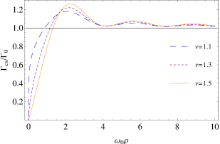
(a) The case for an atom polarizable along the radial direction.

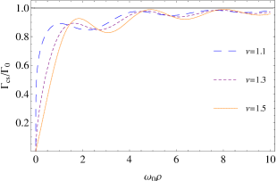
(b) The case for an atom polarizable along the tangential direction.

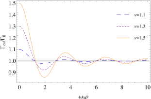
(c) The case for an atom polarizable parallel to the string.

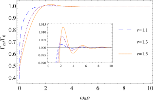
(d) The case for an atom polarizable isotropically.

Figure 1: Ratio between the rate of change of a two-level static atom in the cosmic string spacetime and that in a free Minkowski spacetime.

As shown in the four figures, the relative rate $\frac{\Gamma_{cs}}{\Gamma_{0}}$ for a static atom generally oscillates with the atom-string distance, and the amplitude of oscillation decreases with increasing atom-string distance. Moreover, the oscillation is more severe for larger $\nu$, i.e., larger deficit in the angle induce more severe oscillation. For a two-level atom polarizable along the radial direction, the rate of change of the atomic energy in the cosmic string spacetime is smaller than that in Minkowski spacetime when the atom is located very close to the string, which means that the atomic energy varies slower than in a free Minkowski spacetime. When the atom-string distance exceeds a critical value, the average rate of change of energy in the cosmic string overtakes that in a free Minkowski spacetime as indicated by that the relative rate now becomes larger than unity (see Figure. 1(a)), although the relative rate still oscillates with the distance. The rate of change of the atomic energy approaches that in a Minkowski spacetime as the atom-string distance becomes larger and larger. For an atom polarizable in the tangential direction, (see Figure. 1(b)), the rate of change of the atomic energy is always smaller than that in a free Minkowski spacetime, and the difference becomes smaller with the increase of the atom-string distance. For an atom polarizable parallel to the string (see Figure. 1(c)), the rate of change of the atomic energy can be larger or smaller than that in a free Minkowski spacetime as the ratio $\frac{\Gamma_{cs}}{\Gamma_{0}}$ oscillates around unity as the atom-string distance varies. Notice that here the numerical results are consistent with our previous analytical analysis on the average rate of change of the energy of an atom located very close to the string in that for an atom polarizable perpendicular to the string, the rate is proportional to $\rho^{2(\nu-1)}\sim 0$, and for an atom polarizable parallel to the string, the rate is proportional to $\nu$. We show also the ratio $\frac{\Gamma_{cs}}{\Gamma_{0}}$ for an isotropically polarizable atom in Figure. 1(d), and one can see that it also oscillates around unity, but the amplitude of oscillation is much smaller than the ratio of an atom polarizable parallel to the string (see Figure. 1(c)).

V CONCLUSIONS

We have studied the average rate of change of a multilevel static atom coupled to quantum electromagnetic field in a thermal bath in the cosmic string spacetime. We separately calculate the contributions of thermal fluctuations of the field and radiation reaction of the atom to the average rate of change of the atomic energy. We analyze the behavior of the transition rates analytically in both the near zone and the far zone and numerically for a generic atom-string distance. We find that the transition rates are crucially dependent on the atom-string distance and polarization of the atom and they in general oscillate as the atom-string distance varies. Moreover, the atomic transition rates in the cosmic string spacetime can be larger or smaller than those in Minkowski spacetime contingent upon the atomic polarization and position, meaning the transition rates can be either enhanced or weakened by the cosmic string. In particular, when located on the string, ground-state atoms can transition to excited states only if they are polarizable parallel to the string, whereas ground state atoms polarizable only perpendicular to the string are stable as if they were in a vacuum, even if they are immersed in a thermal bath. This feature can be attributed to the fact that on the string, only the $z-$component of the electric field is nonzero and it is reminiscent of a perfect conducting boundary where only component of the electric field which is perpendicular to the surface is non-zero. In this sense, the effect of a cosmic string is very similar to that of a perfect conducting boundary. This does not come as a surprise since the cosmic string only modifies the global spacetime topology while leaving the local space flatness intact in a similar way as what a conducting boundary does to a flat space.

References

(1) T. A. Welton, Phys. Rev. 74, 1157 (1948).
(2) G. Compagno, R. Passante and F. Persico, Phys. Lett. A 98, 253 (1983).
(3) J. R. Ackerhalt, P. L. Knight and J. H. Eberly, Phys. Rev. Lett. 30, 456 (1973).
(4) P. W. Milonni, Phys. Scr. 21, 102 (1988).
(5) P. W. Milonni and W. A. Smith, Phys. Rev. A 11, 814 (1975).
(6) J. H. van Vleck, Phys. Rev. 24, 330 (1924).
(7) P. A. M. Dirac, Pro. Roy. Soc. Lond. A 114, 243 (1927).
(8) I. R. Senitzky, Phys. Rev. Lett. 31, 955 (1973).
(9) P. W. Milonni, J. R. Ackerhalt and W. A. Smith, Phys. Rev. Lett. 31, 958 (1973).
(10) J. R. Ackerhalt and J. H. Eberly, Phys. Rev. D 10, 3350 (1974).
(11) P. W. Milonni, Phys. Rep. 25, 1 (1975).
(12) J. Dalibard, J. Dupont-Roc, and C. Cohen-Tannoudji, J. Phys. (Paris) 43, 1617 (1982); ibid, 45, 637 (1984).
(13) J. Audretsch and R. Müller, Phys. Rev. A 50, 1755 (1994); ibid, 52, 629 (1995).
(14) J. Audretsch, R. Müller, and M. Holzmann, Class. Quant. Grav. 12, 2927 (1995).
(15) R. Passante, Phys. Rev. A 57, 1590 (1998).
(16) H. Yu and S. Lu, Phys. Rev. D 72, 064022 (2005).
(17) Z. Zhu, H. Yu and S. Lu, Phys. Rev. D 73, 107501 (2006).
(18) Z. Zhu and H. Yu, Phys. Rev. D 74, 044032 (2006).
(19) Z. Zhu and H. Yu, Phys. Lett. B 645, 459 (2007).
(20) L. Rizzuto, Phys. Rev. A 76, 062114 (2007).
(21) L. Rizzuto and S. Spagnolo, Phys. Rev. A 79, 062110 (2009);
ibid, J. Phys.: Conf. Ser. 161, 012031 (2009).
(22) Z. Zhu and H. Yu, Phys. Rev. A 82, 042108 (2010).
(23) L. Rizzuto and S. Spagnolo, Phys. Scr., T 143, 014021 (2011).
(24) W. Zhou and H. Yu, Phys. Rev. A 86, 033841 (2012).
(25) J. L. Tomazelli and L. C. Costa, Int. J. Mod. Phys. A 18, 1079 (2003).
(26) Z. Zhu and H. Yu, Phys. Rev. A 79, 032902 (2009);
ibid, Phys. Rev. A 86, 052508 (2012).
(27)W. She, H. Yu and Z. Zhu, Phys. Rev. A 81, 012108 (2010).
(28) L. Iliadakis, U. Jasper, and J. Audretsch, Phys. Rev. D 51, 2591 (1995).
(29) W. Zhou and H. Yu, JHEP 4, 024 (2007); H. Yu and W. Zhou, Phys. Rev. D 76, 027503 (2007); ibid, 76, 044023 (2007).
(30) Z. Zhu and H. Yu, JHEP 2, 033 (2008).
(31) W. Zhou and H. Yu, Class. Quant. Grav. 29, 085003 (2012); ibid, JHEP 10, 172 (2012).
(32) A. Vilenkin, Phys. Rev. D 23, 852 (1981).
(33) A. N. Aliev and D. V. Gal’tsov, Ann. Phys., NY 193, 142 (1989).
(34) A. N. Aliev, Class. Quant. Grav. 10, 2531 (1993).
(35) A. A. Saharian, A. S. Kotanjyan, Phys. Lett. B 713, 133 (2012); ibid, Eur. Phys. J. C 71, 1765 (2011).
(36) E. R. Bezerra de Mello, A. A. Saharian, and A. Kh. Grigoryan, J. Phys. A: Math. Theor. 45, 374011 (2012).
(37) E. R. Bezerra de Mello, V. B. Bezerra, H. F. Mota and A. A. Saharian, Phys. Rev. D 86, 065023 (2012).
(38) L. Iliadakis, U. Jasper, and J. Audretsch, Phys. Rev. D 51, 2591 (1995).
(39) V. D. Skarzhinsky, D. D. Harari, and U. Jasper, Phys. Rev. D 49, 755 (1994).