Massive quiver matrix models for massive charged particles in AdS

Abstract

We present a new class of ${\cal N}=4$ supersymmetric quiver matrix models and argue that it describes the stringy low-energy dynamics of internally wrapped D-branes in four-dimensional anti-de Sitter (AdS) flux compactifications. The Lagrangians of these models differ from previously studied quiver matrix models by the presence of mass terms, associated with the AdS gravitational potential, as well as additional terms dictated by supersymmetry. These give rise to dynamical phenomena typically associated with the presence of fluxes, such as fuzzy membranes, internal cyclotron motion and the appearance of confining strings. We also show how these models can be obtained by dimensional reduction of four-dimensional supersymmetric quiver gauge theories on a three-sphere.

1 Introduction and summary

Type II string theory compactified on a six-dimensional manifold $X_{6}$ gives rise to a four-dimensional spacetime $M_{4}$. A D$p$-brane wrapped on a $p$-dimensional cycle in $X_{6}$ appears as a charged particle in $M_{4}$. The wrapped branes interact with each other via strings that end on them. At small separations, the lightest open string modes dominate the interactions. The low-energy dynamics of these modes is captured by quiver matrix mechanics Douglas:1996sw; Douglas:1996yp; Douglas:2000qw; Denef:2002ru. A quiver is an oriented graph of which the vertices are called nodes and the edges arrows. In quiver matrix mechanics, the nodes correspond to four-dimensional spacetime degrees of freedom and label wrapped branes; the arrows correspond to internal-space degrees of freedom and label open string modes. If $X_{6}$ is a Calabi-Yau manifold without fluxes then $M_{4}$ is flat Minkowski space and the bulk superalgebra has eight supercharges, of which the branes preserve four. In this case, the corresponding one-dimensional ${\cal N}=4$ quiver matrix mechanics Lagrangian may be obtained by dimensional reduction of a four-dimensional ${\cal N}=1$ quiver gauge theory. On the other hand if $X_{6}$ is an Einstein manifold carrying magnetic fluxes, compactifications with eight or more supersymmetries to $M_{4}={\rm AdS}_{4}$ are possible. A standard example is the type IIA ${\rm AdS}_{4}\times{\mathbb{C}P}^{3}$ compactification Watamura:1983hj; Nilsson:1984bj holographically dual to ABJM theory Aharony:2008ug. Thus, a natural question is what the analogous quiver matrix mechanics description is for D-particles in ${\rm AdS}_{4}$. In this paper we answer this question.

We will argue that the low energy, short distance dynamics of particles in AdS₄, obtained as internally wrapped branes preserving at least four supercharges, is captured by a tightly constrained ${\cal N}=4$ supersymmetric massive quiver matrix mechanics. By “massive” we mean the brane position degrees of freedom are trapped near the origin by a harmonic potential, interpreted here as the AdS gravitational potential well. These ${\cal N}=4$ massive quiver matrix models generalize the ${\cal N}=16$ BMN matrix model Berenstein:2002jq, which is a mass deformation of the BFSS matrix model Banks:1996vh. Although the standard interpretation of the BMN model is quite different from the interpretation we consider here, its Lagrangian can nevertheless be viewed a special case of our general class of models, after a suitable field redefinition. As was pointed out in Kim:2003rza, the BMN model can be obtained by dimensionally reducing ${\cal N}=4$ super-Yang-Mills theory on ${\mathbb{R}}\times S^{3}$. Similarly, we will see that the ${\cal N}=4$ massive quiver matrix models we present can be obtained by dimensional reduction of ${\cal N}=1$ quiver gauge theories on ${\mathbb{R}}\times S^{3}$. The details of this reduction are given in section LABEL:sec:reduction.

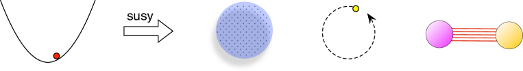
Figure 1: Our results in pictures: mass deformation with four supercharges implies flux phenomena such as fuzzy membranes, internal space cyclotron motion, and branes confined by strings. We will elaborate on these in the introduction and especially in sections LABEL:sec:interpads, LABEL:sec:NAMyers, LABEL:sec:internalmagnetic, and LABEL:sec:gaussconfines, respectively.

The core result of the paper is the general Lagrangian of these ${\cal N}=4$ massive quiver matrix models, presented in section 2. Besides the parameters already present in the flat-space quiver mechanics of Denef:2002ru (particle masses $m_{v}$, Fayet-Ilopoulos parameters $\theta_{v}$ and superpotential data), they depend on just one additional mass deformation parameter $\Omega$, appearing in harmonic potentials for the particle positions $\vec{x}_{v}$,

$$V(x)=\sum_{v}\tfrac{1}{2}m_{v}\,\Omega^{2}\,\vec{x}_{v}^{2}\,,$$ (1)

as well as in a number of other terms related by supersymmetry. The parameter $\Omega$ has the dimension of frequency. In the context of our AdS interpretation, it equals the global time oscillation frequency of a particle in the AdS gravitational well:

$$\Omega=\frac{c}{\ell_{\rm AdS}}\,,$$ (2)

where $c$ is the speed of light and $\ell_{\mathrm{AdS}}$ is the AdS radius. Under some simplifying assumptions stated in section 2, we conjecture that this captures, in fact, the most general case consistent with the symmetries imposed. In the context of the AdS interpretation, the isotropic harmonic potential is due to the AdS gravitational potential well. The fact that the deformation introduces just one new parameter, uniform across all connected nodes, can be physically understood as the equality of gravitational and inertial mass, i.e., the equivalence principle. In view, however, of the very different (short distance) regime of validity of the quiver picture and the (long distance) bulk supergravity picture, it is by no means a priori obvious that the quiver should retain this feature of gravity. It does so as a consequence of the structure of the interactions and the constraints of supersymmetry.

Further remarkable consequences are highlighted in figure 1. Turning on the mass deformation for the position degrees of freedom and requiring ${\cal N}=4$ supersymmetry automatically implies all of the peculiar dynamical phenomena typically featured by branes in flux backgrounds, including noncommutative fuzzy membranes, magnetic cyclotron motion in the internal space, and confinement of particles by fundamental strings. In section LABEL:sec:examples we discuss examples explicitly exhibiting these phenomena in simple quiver models. The supergravity counterpart of this is, essentially, that supersymmetric compactifications to AdS require flux Duff:1986hr; Grana:2005jc; Douglas:2006es.

We devote particular attention to the emergence of confining strings, as this is perhaps the most dramatic difference with the flat-space quiver models of Denef:2002ru, and one of the main motivations for this work, prompted by problems raised in Anninos:2013mfa. The goal of Anninos:2013mfa was to demonstrate the existence of multicentered black hole bound states in AdS₄ flux compactifications and to investigate their potential use as holographic models of structural glasses. A simple four-dimensional gauged supergravity model was considered, with the appropriate ingredients needed to lift previously known, asymptotically flat bound states of black holes carrying wrapped D-brane charges Denef:2000nb; Denef:2002ru; Denef:2007vg; Anninos:2011vn to AdS₄ with minimal modifications. However, as was pointed out already in Anninos:2013mfa, this model actually misses an important universal feature of flux compactifications of string theory; the fact that particles obtained by wrapping branes on certain cycles are confined by fundamental strings.

In the example of AdS${}_{4}\times{\mathbb{C}P}^{3}$, dual to ABJM theory, it was explained in Aharony:2008ug how this can be understood from a four-dimensional effective field theory point of view; it is because these particles have a nonzero magnetic charge with respect to a Higgsed $\mathrm{U}(1)$. The Higgs condensate forces the magnetic flux lines into flux tubes, which act as confining strings. Alternatively, their inevitability can be inferred directly from the D-brane action. In the presence of background flux, the Gauss’s law constraint for the brane worldvolume gauge field gets a contribution equal to the quantized flux threading the brane, which must be canceled by an equal amount of endpoint charge of fundamental strings attached to the brane. This shows that the confining strings are fundamental strings, and a rather universal feature of flux compactifications. If the brane is considered in isolation, the attached strings extend out from it all the way to the boundary of AdS. For this reason, such branes are often called baryonic vertices Witten:1998xy. Note, however, that suitable pairs of charges may allow the strings emanating from one brane to terminate on the other, thus producing a finite-energy configuration.

In section LABEL:sec:two_nodes we show that all of this is elegantly reproduced by massive quiver matrix mechanics. Gauss’s law for the quiver gauge fields forces charged fields to have a nonzero minimal excitation energy that grows linearly with particle separation. The tension of this string is a multiple of the fundamental string tension. More precisely, the number of fundamental strings $N_{F,v}$ terminating on a brane corresponding to a quiver node $v$, with Fayet-Iliopoulos (FI) parameter $\theta_{v}$, is given by the universal formula

$$N_{F,v}=\Omega\,\theta_{v}\,.$$ (3)

Quantum consistency requires $N_{F,v}$ to be an integer and hence $\theta_{v}$ to be quantized, in contrast to the case of flat-space quivers, where the FI parameters are related to continuously tunable bulk moduli. This is consistent with the fact that bulk moduli are typically stabilized in flux compactifications. As in the flat space case, the FI parameters also control supersymmetric bound state formation. In particular, for a two-node quiver with all arrows oriented in one direction, a supersymmetric bound state exists for one sign of the FI parameter but not the other. An interesting immediate consequence is that the boundary of the region in constituent charge space where supersymmetric bound states cease to exist is the same as the codimension-one slice through charge space where confining strings between the constituents are absent. In section LABEL:sec:ABJM we interpret these findings in some detail for internally wrapped branes in AdS${}_{4}\times{\mathbb{C}P}^{3}$.

Most of the analysis in this paper is classical, but we provide the complete quantum Hamiltonian and supersymmetry algebra in appendix LABEL:app:algebra. The supersymmetry algebra is $\mathfrak{su}(2|1)$. If the Lagrangian has a $\mathrm{U}(1)_{R}$ symmetry, the algebra is extended to the semidirect product $\mathfrak{su}(2|1)\rtimes\mathfrak{u}(1)_{R}$. This algebra arises naturally on the worldline of a superparticle in an ${\cal N}=2$ AdS₄ background, as shown in appendix LABEL:app:osp2bar4. This confirms our AdS interpretation and provides the appropriate identifications of the global AdS energy with a particular linear combination of the Hamiltonian and the $R$-charge generator, namely the global AdS $R$-frame identified in section LABEL:sec:energydef.

We note that the chiral multiplet part of the massive quiver matrix mechanics Lagrangian in equation (4) has been given before, as part of a systematic construction of supersymmetric quantum mechanics models with $\mathfrak{su}(2|1)$ supersymmetry Ivanov:2014ima; Ivanov:2013ova. This part can also be obtained by dimension reduction of the general four-dimensional ${\cal N}=1$ chiral multiplet Lagrangian of Festuccia:2011ws on ${\mathbb{R}}\times S^{3}$, and it has been obtained this way in Assel:2015nca, for the purpose of computing Casimir energies in conformal field theories on curved spaces. The dimensional reduction of the four-dimensional vector multiplet is also known from Kim:2003rza, but we explain how to create a general gauged $\mathfrak{su}(2|1)$ quantum mechanics with coupled vector and chiral multiplets and an arbitrary superpotential. The massive quiver Lagrangian in equation (4) is a special case of these models as is the BMN matrix model (see LABEL:sec:BMN). We explain how to perform the dimensional reduction in section LABEL:sec:reduction and give additional details in appendix LABEL:app:reductiondetails. In section LABEL:sec:reduccomparison, we give a more detailed comparison of our models and those given in the works Ivanov:2014ima; Ivanov:2013ova.

2 General Lagrangian and supersymmetry

In this section we give the core results of the paper, the general massive quiver matrix mechanics Lagrangian and its supersymmetries. It represents a general deformation of the quiver models of Denef:2002ru (see especially appendix C) preserving $\mathrm{SO}(3)$ rotation symmetry and ${\cal N}=4$ supersymmetry. For simplicity, we also restrict to a flat target-space metric for both the vector and chiral multiplets. We conjecture that this is the most general Lagrangian having these properties.

The field content remains the same as in Denef:2002ru. It is encoded in a quiver, with nodes $v\in V$, directed edges (arrows) $a\in A$, and dimension vector $N=(N_{v})_{v\in V}$. To each node is assigned a vector, or linear, multiplet $(A_{v},\leavevmode\nobreak\ X_{v}^{i},\leavevmode\nobreak\ {\lambda_{v}}_{\alpha},\leavevmode\nobreak\ D_{v})$ with $i=1,\leavevmode\nobreak\ 2,\leavevmode\nobreak\ 3$. The field $A_{v}$ is the gauge field for the group $\mathrm{U}(N_{v})$. The fields $X_{v}^{i}$, ${\lambda_{v}}_{\alpha}$, $D_{v}$ transform in the adjoint of $\mathrm{U}(N_{v})$. To each edge $a:v\rightarrow w$ is assigned a chiral multiplet $(\phi^{a},\leavevmode\nobreak\ \psi^{a}_{\alpha},\leavevmode\nobreak\ F^{a})$ transforming in the bifundmental $(N_{w},\bar{N}_{v})$ of $\mathrm{U}(N_{w})\times\mathrm{U}(N_{v})$. In a string theory context the nodes $v$ can be thought of as labeling different “parton” D-branes wrapped on internal cycles with multiplicity $N_{v}$, and arrows $a:v\to w$ as labeling light open string modes polarized in the internal dimensions, connecting the parton branes.

The Lagrangian depends on a number of parameters that are already present in the flat-space quiver models. For each node $v$, there is an inertial mass parameter $m_{v}$ determining the kinetic terms for the vector multiplet fields, and a Fayet-Iliopoulos (FI) parameter $\theta_{v}$ setting the D-term potential for the scalars $\phi^{a}$ connected to the node $v$. The quiver model may also have a superpotential, given by an arbitrary gauge-invariant holomorphic function $W(\phi^{a})$ of the $\phi^{a}$.

Before imposing any supersymmetry, a general SO(3)-symmetric and gauge invariant mass deformation of the vector multiplets consists of adding harmonic potential terms of the form $\frac{\mu_{v}}{2}{\rm Tr}(X^{i}_{v})^{2}$ to the Lagrangian, and similarly for the fermions. Requiring ${\cal N}=4$ supersymmetry to be preserved dictates the inclusion of additional terms for the vector and chiral multiplets, and reduces the a priori arbitrary deformation parameters $\mu_{v}$ to functions of a single deformation parameter $\Omega$, namely $\mu_{v}=m_{v}\,\Omega^{2}$. In the AdS interpretation discussed in section LABEL:sec:examples, we identify $\Omega=1/\ell_{\rm AdS}$. In appendix LABEL:app:susy, we provide more details on how supersymmetry fixes the form of the mass deformation. In section LABEL:sec:reduction, we explain how it can be obtained from dimensional reduction of ${\cal N}=1$ quiver gauge theories on ${\mathbb{R}}\times S^{3}$.

2.1 Lagrangian

The Lagrangian of massive quiver matrix mechanics with deformation parameter $\Omega$ is given by

$$\mathcal{L}_{\Omega}=\mathcal{L}^{0}+\mathcal{L}^{\prime}_{\Omega}\ ,$$ (4)

where $\mathcal{L}^{0}$ is the original, undeformed, flat-space quiver Lagrangian, identical to the Lagrangian in appendix C of Denef:2002ru, and $\mathcal{L}^{\prime}_{\Omega}$ is the mass deformation. We give our conventions and definitions for this Lagrangian in detail in appendix LABEL:app:Def.

$$\mathcal{L}^{0} =\mathcal{L}_{V}^{0}+\mathcal{L}_{FI}^{0}+\mathcal{L}_{C}^{0}+\mathcal{L}_{I}^{0}+\mathcal{L}_{W}^{0}$$ (5)

$$\mathcal{L}_{V}^{0} =\sum_{v}m_{v}\text{Tr}\left(\tfrac{1}{2}(\mathcal{D}_{t}X_{v}^{i})^{2}+\tfrac{1}{2}D_{v}^{2}+\tfrac{1}{4}[X^{i}_{v},X^{j}_{v}]^{2}+\tfrac{i}{2}(\lambda^{\dagger}_{v}\mathcal{D}_{t}\lambda_{v}-(\mathcal{D}_{t}\lambda^{\dagger}_{v})\lambda_{v})-\lambda^{\dagger}_{v}\sigma^{i}[X^{i}_{v},\lambda_{v}]\right)$$

$$\mathcal{L}_{FI}^{0} =-\sum_{v}\theta_{v}\text{Tr}D_{v}$$

$$\mathcal{L}_{C}^{0} =\sum_{a}\text{Tr}\left(|\mathcal{D}_{t}\phi^{a}|^{2}+|F^{a}|^{2}+\tfrac{i}{2}(\psi^{a{\dagger}}\mathcal{D}_{t}\psi^{a}-(\mathcal{D}_{t}\psi^{a{\dagger}})\psi^{a})\right)$$

$$\mathcal{L}_{W}^{0} =\sum_{a}\text{Tr}\left(\frac{\partial W}{\partial\phi^{a}}F^{a}+\text{h.c.}\right)+\sum_{ab}\text{Tr}\left(\frac{1}{2}\frac{\partial^{2}W}{\partial\phi^{a}\partial\phi^{b}}\psi^{b}\epsilon\psi^{a}+\text{h.c.}\right)$$

$$\mathcal{L}_{I}^{0} =-\sum_{a:v\rightarrow w}\text{Tr}\bigl{(}(\phi^{a{\dagger}}X_{w}^{i}-X_{v}^{i}\phi^{a{\dagger}})(X_{w}^{i}\phi^{a}-\phi^{a}X_{v}^{i})-\phi^{a{\dagger}}(D_{w}\phi^{a}-\phi^{a}D_{v})$$

$$\qquad+\psi^{a{\dagger}}\sigma^{i}(X^{i}_{w}\psi^{a}-\psi^{a}X^{i}_{v})+i\sqrt{2}\left((\phi^{a{\dagger}}\lambda_{w}-\lambda_{v}\phi^{a{\dagger}})\epsilon\psi^{a}-\psi^{a{\dagger}}\epsilon(\lambda_{w}^{\dagger}\phi^{a}-\phi^{a}\lambda^{\dagger}_{v})\right)\bigr{)}$$

$$\mathcal{L}^{\prime}_{\Omega} =\mathcal{L}_{V}^{\prime}+\mathcal{L}_{FI}^{\prime}+\mathcal{L}_{C}^{\prime}$$ (6)

$$\mathcal{L}_{V}^{\prime} =-\sum_{v}m_{v}\text{Tr}\left(\tfrac{1}{2}\,\Omega^{2}(X_{v}^{i})^{2}+\tfrac{3}{2}\,\Omega\,\lambda^{\dagger}_{v}\lambda_{v}+i\,\Omega\,\epsilon_{ijk}X_{v}^{i}X_{v}^{j}X^{k}_{v}\right)$$

$$\mathcal{L}_{FI}^{\prime} =\sum_{v}\theta_{v}\,\Omega\,\text{Tr}A_{v}$$

$$\mathcal{L}_{C}^{\prime} =\sum_{a}\text{Tr}\left(\tfrac{i}{2}\,\Omega\bigl{(}(\mathcal{D}_{t}\phi^{a\dagger})\phi^{a}-\phi^{a\dagger}\mathcal{D}_{t}\phi^{a}\bigr{)}-\tfrac{1}{2}\,\Omega\,\psi^{a{\dagger}}\psi^{a}\right)\,.$$

The covariant derivatives are given by

$$\mathcal{D}_{t}X_{v}^{i} =\partial_{t}X_{v}^{i}-i[A_{v},X_{v}^{i}],$$

$$\mathcal{D}_{t}\lambda_{v} =\partial\lambda_{v}-i[A_{v},\lambda_{v}],\quad\mathcal{D}_{t}\lambda_{v}^{\dagger}=\partial\lambda_{v}^{\dagger}-i[\lambda_{v}^{\dagger},A_{v}],$$

$$\mathcal{D}_{t}\phi^{a} =\partial_{t}\phi^{a}-iA_{w}\phi^{a}+i\phi^{a}A_{v},\quad\mathcal{D}_{t}\phi^{a{\dagger}}=\partial_{t}\phi^{a{\dagger}}+i\phi^{a{\dagger}}A_{w}-iA_{v}\phi^{a{\dagger}}$$

$$\mathcal{D}_{t}\psi^{a} =\partial_{t}\psi^{a}-iA_{w}\psi^{a}+i\psi^{a}A_{v},\quad\mathcal{D}_{t}\psi^{a{\dagger}}=\partial_{t}\psi^{a{\dagger}}+i\psi^{a{\dagger}}A_{w}-iA_{v}\psi^{a{\dagger}},$$

with the arrow $a:v\to w$.

2.2 Supersymmetry transformations

The action is supersymmetric with respect to the transformations ΔδA_v &= iλ^†_vξ- iξ^†λ_v
δX_v^i = iλ^†_vσ^iξ- iξ^†σ^iλ_v
δλ_v = (D_tX^i_v)σ^iξ+12ϵ^ijk[X^i_v,X^j_v]σ^kξ+ iD_vξ- i   Ω  X^i_vσ^iξ
δD_v = -(D_tλ_v^†)ξ- i[X_v^i,λ^†_v]σ^iξ- ξ^†(D_tλ_v) - iξ^†σ^i[X^i_v,λ_v]   + 3i2   Ω  λ_v^†ξ- 3i2   Ω  ξ^†λ_v
δϕ^a = -2  ξϵψ^a
δψ^a = -i2  ξ^†ϵ(D_tϕ^a) - 2  σ^i(ξ^†ϵ)(X^i_wϕ^a - ϕ^aX_v^i) + 2  ξF^a
δF^a = -i2  ξ^†(D_tψ^a) + 2  ξ^†σ^i(X^i_wψ^a - ψ^aX_v^i) - 2iξ^†ϵ(λ