Accelerating the Uzawa Algorithm

Abstract

The Uzawa algorithm is an iterative method for the solution of saddle-point problems, which arise in many applications, including fluid dynamics. Viewing the Uzawa algorithm as a fixed-point iteration, we explore the use of Anderson acceleration (also known as Anderson mixing) to improve the convergence. We compare the performance of the preconditioned Uzawa algorithm with and without acceleration on several steady Stokes and Oseen problems for incompressible flows. For perspective, we include in our comparison GMRES with two different preconditioners. The results indicate that the accelerated preconditioned Uzawa algorithm converges significantly faster than the algorithm without acceleration and is competitive with the other methods considered.

siscxxxxxxxx–x

1 Introduction

A saddle-point problem is a block 2$\times$2 linear system of the form

(7) $$\underbrace{\left(\begin{array}[]{cc}{A}&{B}^{T}\\ {B}&C\end{array}\right)}_{\mathcal{A}}\left(\begin{array}[]{c}{u}\\ p\end{array}\right)=\underbrace{\left(\begin{array}[]{c}{f}\\ g\end{array}\right)}_{b}.$$

Here, $A$ is assumed to be invertible but may be symmetric or non-symmetric. Applications in which saddle-point problems arise include computational fluid dynamics [27, 35], constrained optimization [41], linear elasticity, economics, and many other areas [8].

Many methods for solving saddle-point problems have been developed and analyzed, including direct and iterative methods (see [8] for an extensive review). Here, we consider the Uzawa algorithm [2], a well-known and easily implemented iterative method. Extensions of the classical Uzawa algorithm include the augmented Lagrangian formulation [11, 33] and the inexact Uzawa algorithm (also known as the Arrow–Hurwicz method) [12, 15, 21, 20, 28, 31, 36, 45]. A relaxation parameter appears in the algorithm, and methods for determining optimal values of this are outlined in [3]. Additionally, the use of preconditioners to increase the speed of convergence of these methods has been studied by a number of authors [12, 13, 15, 17, 21, 20, 29].

In practice, the iterates produced by the Uzawa algorithm often converge undesirably slowly. In this paper, we view the algorithm as a fixed-point iteration and consider the use of Anderson acceleration [1], also known as Anderson mixing, to improve the convergence. This acceleration method (denoted henceforth by AA) has enjoyed considerable success in accelerating fixed-point iterations in electronic-structure computations (see [25] and the references therein), simulations of transport phenomena [14, 30], and coupled fluid-solid interface problems [26]. It has also been effective in accelerating Picard iterations in variably saturated flow simulations [34] and advection-diffusion problems [32]. To the best of our knowledge, it has not been previously used with the Uzawa algorithm or other iterations for saddle-point problems.

It is unusual to apply AA in the context of a linear problem such as (7), for which there are many possible alternative solution methods. Indeed, as we note below, AA coupled with the Uzawa algorithm is very closely related to GMRES [37] with a certain preconditioning applied to (7). Our goal is to present AA as an easily implemented and economical way to mitigate the often slow convergence of Uzawa iterates and to demonstrate the performance of the accelerated algorithm on several model problems.

In the following, we focus on applying AA to the Uzawa algorithm for the Stokes and Oseen problems of steady incompressible flow. The use of AA with any iterative method in this fluids setting appears to be new. In this context, $C=0$ in (7) when applying a stable finite-element discretization. (The extension to non-zero $C$ is straightforward.) We briefly consider the classical standard form of the Uzawa algorithm but focus primarily on the preconditioned form, since the standard form without preconditioning converges too slowly to be practical on the problems of interest. In Section 2, we outline the standard and preconditioned algorithms. In Section 3, we first note a particular way in which the Uzawa algorithm can be recast as a fixed-point iteration; we then describe AA and discuss its relationship with GMRES in this case. In Section 4, we report on numerical experiments, in which we compare the performance of the Uzawa algorithm, with and without acceleration, in several Stokes and Oseen flow scenarios. For perspective, we include the closely related preconditioned GMRES method and also, in most tests, GMRES preconditioned with the Relaxed Dimensional Factorization (RDF) preconditioner developed in [10]. In Section 5, we offer a summary discussion and conclusions.

2 Variations of the Uzawa algorithm

2.1 Standard Uzawa

The standard Uzawa algorithm consists of a coupled iteration for the variables $p$ and $u$. Given an initial guess for $p_{0}$, the iteration is

(8a) $$u_{k+1} =A^{-1}(f-B^{T}p_{k}),$$

(8b) $$p_{k+1} =p_{k}+\omega(Bu_{k+1}-g),$$

where $\omega>0$ is a relaxation parameter. It has been previously shown that if one eliminates $u_{k+1}$ from (8b) by using (8a), then the Uzawa method is equivalent to a Richardson iteration, which can be used to determine an optimal $\omega$ in terms of the maximum and minimum eigenvalues of the Schur complement $\mathcal{S}=BA^{-1}B^{T}$ [21]. Bounds obtained in [21] suggest that the iterates will converge slowly if the Schur complement is not well conditioned. Several variations of this standard algorithm have been developed, including preconditioned versions that we will describe next.

2.2 Preconditioned Uzawa

We consider the preconditioned Uzawa algorithm in the general form given in [12]:

(9a) $${u_{k+1}} =u_{k}+Q_{A}^{-1}\left({f-(Au_{k}+B^{T}p_{k}})\right),$$

(9b) $$p_{k+1} =p_{k}+\omega Q_{B}^{-1}(Bu_{k+1}-g),$$

where $Q_{A}$ and $Q_{B}$ are preconditioners. When $Q_{A}=A$, this becomes the preconditioned Uzawa algorithm considered in [21]; when $Q_{B}=I$ as well, it reduces to the standard Uzawa algorithm in (8a)$-$(8b). Note also that (9a)$-$(9b) require an initial guess for $u_{0}$ as well as $p_{0}$ if $Q_{A}\neq A$.

Often, $A$ is symmetric positive-definite (SPD). In this case, suitable preconditioners $Q_{A}$ and $Q_{B}$ should be SPD as well, and various choices have appeared in the literature. For example, [21] includes an instance of (9a)$-$(9b) with $Q_{A}=A$ and $Q_{B}$ a scaled diagonal or tridiagonal matrix derived from the mass matrix of a finite-element discretization. Other examples appear in [12], with $Q_{A}$ a multigrid V-cycle and $Q_{B}=I$, and in [15], with $Q_{A}$ an incomplete-Cholesky factorization of $A$ and $Q_{B}$ a scaled identity matrix. Choices of $Q_{A}$ and $Q_{B}$ when $A$ is non-symmetric are similarly varied. For example, in both [13] and [17], the symmetric part $A_{S}={{1}\over{2}}(A+A^{T})$ is assumed to be SPD. Choices of $Q_{A}$ and $Q_{B}$ in [13] include taking $Q_{A}$ to be a multigrid V-cycle on $A_{S}$ and $Q_{B}$ to be a scaled identity matrix; choices in [17] include $Q_{A}=A$ and $Q_{B}=B(A_{S})^{-1}B^{T}$.

3 Accelerating preconditioned Uzawa

Although the developments in this section are for the preconditioned Uzawa algorithm (9a)–(9b), it is straightforward to adapt them to the standard algorithm (8a)–(8b) by taking $Q_{A}=A$ and $Q_{B}=I$.

3.1 Preconditioned Uzawa as a fixed-point iteration

We begin by rewriting the preconditioned Uzawa algorithm as a fixed-point iteration. From (9a)–(9b), we have

(10) $$\underbrace{\left(\begin{array}[]{cc}Q_{A}&0\\ B&-\frac{1}{\omega}Q_{B}\end{array}\right)}_{\mathcal{M}}\left(\begin{array}[]{c}u_{k+1}\\ p_{k+1}\end{array}\right)=\underbrace{\left(\begin{array}[]{cc}Q_{A}-A&-B^{T}\\ 0&-\frac{1}{\omega}Q_{B}\end{array}\right)}_{\mathcal{N}}\left(\begin{array}[]{c}u_{k}\\ p_{k}\end{array}\right)+\left(\begin{array}[]{c}f\\ g\end{array}\right),$$

which immediately gives the following fixed-point version of preconditioned Uzawa:

(11) $$\left(\begin{array}[]{c}u_{k+1}\\ p_{k+1}\end{array}\right)=G\left(\begin{array}[]{c}u_{k}\\ p_{k}\end{array}\right)\equiv\mathcal{M}^{-1}\left(\mathcal{N}\left(\begin{array}[]{c}u_{k}\\ p_{k}\end{array}\right)+\left(\begin{array}[]{c}f\\ g\end{array}\right)\right).$$

The explicit form of the right hand side of (11) is

$$\left(\begin{array}[]{cc}Q^{-1}_{A}(Q_{A}-A)&-Q_{A}^{-1}B^{T}\\[4.0pt] \omega Q_{B}^{-1}BQ_{A}^{-1}(Q_{A}-A)&I-\omega Q_{B}^{-1}BQ^{-1}_{A}B^{T}\end{array}\right)\left(\begin{array}[]{c}u_{k}\\ p_{k}\end{array}\right)+\left(\begin{array}[]{c}Q_{A}^{-1}f\\[4.0pt] \omega Q_{B}^{-1}(BQ_{A}^{-1}f-g)\end{array}\right),$$

where $BQ_{A}^{-1}B^{T}$ is an approximation of the Schur complement $BA^{-1}B^{T}$. In the case $Q_{A}=A$, the form of (11) is

(12) $$\left(\begin{array}[]{c}u_{k+1}\\ p_{k+1}\end{array}\right)=\left(\begin{array}[]{cc}0&-A^{-1}B^{T}\\[2.0pt] 0&I-\omega Q_{B}^{-1}BA^{-1}B^{T}\end{array}\right)\left(\begin{array}[]{c}u_{k}\\ p_{k}\end{array}\right)+\left(\begin{array}[]{c}A^{-1}f\\[2.0pt] \omega Q_{B}^{-1}(B{A}^{-1}f-g)\end{array}\right).$$

Formally, the iteration (12), like (11), requires an initial guess for $u_{0}$ as well as $p_{0}$. However, in (12), this can be arbitrary.

3.2 Anderson acceleration

The outline of AA given below applies to a general fixed-point iteration $\xi_{i+1}=G(\xi_{k})$ that begins with some initial value $\xi_{o}$. In the context of interest, $\xi=(u,\hskip 2.84544ptp)^{T}$ and $G$ is defined in (11). In the algorithm, $m$ denotes the maximum number of the stored residuals, which is necessarily finite in practice.

Anderson Acceleration

Given $$\xi_{0} m\geq 1 \xi_{1}=G(\xi_{0})$$ and , set .

$$\text{For }k=1,2,...$$

$$\hskip 28.45274pt\text{ Set }m_{k}=\min\{m,k\}.$$

$$\hskip 28.45274pt\text{ Set }F_{k}=(\tilde{f}_{k-m_{k}},\cdots,\tilde{f}_{k}),\text{ where }\tilde{f}_{i}=G(\xi_{i})-\xi_{i}.$$

$$\hskip 28.45274pt\text{ Determine }\alpha^{(k)}=\left(\alpha^{(k)}_{0},\cdots,\alpha^{(k)}_{m_{k}}\right)^{T}\text{ that solves }$$

$$\hskip 56.9055pt\min_{\alpha=(\alpha_{0},\cdots,\alpha_{m_{k}})^{T}}\|F_{k}\alpha\|_{2}\hskip 14.22636pt\text{ s.t. }\hskip 14.22636pt\sum_{i=0}^{m_{k}}\alpha=1.$$

$$\hskip 28.45274pt\text{ Set }\xi_{k+1}=\sum_{i=0}^{m_{k}}\alpha_{i}^{(k)}G(\xi_{k-m_{k}+i}).$$

The rationale underlying AA is that, on a linear fixed-point problem such as the problem of interest here, one has $\sum_{i=0}^{m_{k}}\alpha_{i}^{(k)}G(\xi_{k-m_{k}+i})=G(\sum_{i=0}^{m_{k}}\alpha_{i}^{(k)}\xi_{k-m_{k}+i})$. It follows that, in this case, $\xi_{k+1}$ is obtained by applying $G$ to the point within the affine subspace containing $\xi_{k}$, …, $\xi_{k-m_{k}}$ that has minimal fixed-point residual.

In practice, the constrained least-squares problem in $m_{k}+1$ variables is usually reformulated as an equivalent unconstrained problem in $m_{k}$ variables. See [25, 40] for a particular reformulation that can be implemented efficiently and, in our experience, has been numerically sound. In any case, as the algorithm proceeds, both the number of stored residual vectors and the amount of arithmetic per iteration increase up to maxima determined by $m$. It is important to note, though, that only a single $G$-evaluation is required at each iteration, as in the underlying fixed-point iteration. Thus the cost of applying AA to a fixed-point iteration is only some additional storage and arithmetic (usually modest in practice); no additional $G$-evaluations are required.

3.3 Matrix-splitting preconditioners

As noted in the introduction, the Uzawa algorithm accelerated with AA is closely related to GMRES applied to (7) with a certain preconditioning. To describe this relationship in more detail, we note that the matrix $\mathcal{A}$ in (7) with $C=0$ can be split as follows:

(13) $$\mathcal{A}=\mathcal{M}-\mathcal{N}=\left(\begin{array}[]{cc}Q_{A}&0\\ B&-\frac{1}{\omega}Q_{B}\end{array}\right)-\left(\begin{array}[]{cc}Q_{A}-A&-B^{T}\\ 0&-\frac{1}{\omega}Q_{B}\end{array}\right),$$

where $\mathcal{M}$ and $\mathcal{N}$ are defined in (10) for $Q_{A}$ and $Q_{B}$ in (9a)–(9b).

The fixed-point form of preconditioned Uzawa (11) is a stationary iteration determined by this splitting. Suppose that AA is applied to this stationary iteration without truncation, i.e., with $m_{k}=k$ at each iteration, so that all previous residuals are used in the least-squares problems. Suppose also that unrestarted GMRES is applied to the left-preconditioned system

(14) $$\mathcal{M}^{-1}\mathcal{A}\left(\begin{array}[]{c}u\\ p\end{array}\right)=\mathcal{M}^{-1}\left(\begin{array}[]{c}f\\ g\end{array}\right),$$

starting from the same initial approximate solution. Denote the $k^{th}$ iterates of the two algorithms by $\xi_{k}^{\rm AA}$ and $\xi_{k}^{\rm GMRES}$, respectively, and denote the $k^{th}$ GMRES residual by $r_{k}^{\rm GMRES}$. Then, provided GMRES does not stagnate before the solution is found, Corollary 2.10 in [40] asserts that the two algorithms are “essentially equivalent” in the sense that, until the solution is found, $\xi_{k}^{\rm GMRES}=\sum_{i=0}^{m_{k}}\alpha_{i}^{(k)}\xi_{i}^{\rm AA}$ and $\xi_{k+1}^{\rm AA}=G(\xi_{k}^{\rm GMRES})$, where $G$ is the fixed-point map in (11).

This “essential equivalence” seldom strictly holds in practice, since it is almost always necessary to truncate AA and to restart GMRES. We explore in Section 4 how well this “essential equivalence” is borne out in the problems of interest there. For the present, we note that

$$\mathcal{M}^{-1}=\left(\begin{array}[]{cc}Q_{A}^{-1}&0\\[4.0pt] \omega Q_{B}^{-1}BQ_{A}^{-1}&-\omega Q_{B}^{-1}\end{array}\right),$$

and so the main requirement of using this preconditioner in GMRES is one solve with each of $Q_{A}$ and $Q_{B}$ per iteration. Additionally, the preconditioned system (14) corresponds to

$$\left(\begin{array}[]{cc}Q_{A}^{-1}A&Q_{A}^{-1}B^{T}\\[4.0pt] \omega Q_{B}^{-1}BQ_{A}^{-1}(A-Q_{A})&\omega Q_{B}^{-1}BQ_{A}^{-1}B^{T}\end{array}\right)\left(\begin{array}[]{c}u\\ p\end{array}\right)=\left(\begin{array}[]{c}Q_{A}^{-1}f\\[4.0pt] \omega Q_{B}^{-1}(B{Q_{A}}^{-1}f-g)\end{array}\right),$$

When $Q_{A}=A$, this simplifies to

(15) $$\left(\begin{array}[]{cc}I&A^{-1}B^{T}\\[2.0pt] 0&\omega Q_{B}^{-1}B{A}^{-1}B^{T}\end{array}\right)\left(\begin{array}[]{c}u\\ p\end{array}\right)=\left(\begin{array}[]{c}A^{-1}f\\[2.0pt] \omega Q_{B}^{-1}(B{A}^{-1}f-g)\end{array}\right).$$

We refer to GMRES applied to (15) as PGMRES in the sequel. When $Q_{A}=A$, it follows from the discussion above that untruncated AA applied to preconditioned Uzawa is “essentially equivalent” in the above-defined sense to unrestarted PGMRES. When $Q_{B}=I$ as well, preconditioned Uzawa reduces to standard Uzawa, and it follows that untruncated AA applied to standard Uzawa is “essentially equivalent” to unrestarted GMRES applied to (15) with $Q_{B}=I$, i.e.,

(16) $$\left(\begin{array}[]{cc}I&A^{-1}B^{T}\\[2.0pt] 0&\omega B{A}^{-1}B^{T}\end{array}\right)\left(\begin{array}[]{c}u\\ p\end{array}\right)=\left(\begin{array}[]{c}A^{-1}f\\[2.0pt] \omega(B{A}^{-1}f-g)\end{array}\right),$$

which mainly requires one solve with $A$ at each iteration.

The forms of (15) and (16) are especially convenient for applying GMRES. For example, the matrix-vector products required for GMRES applied to (15) mainly require only one solve with each of $A$ and $Q_{B}$, in addition to matrix-vector products with $B$ and $B^{T}$. Alternatively, one may prefer first to solve the preconditioned or unpreconditioned Schur-complement system, i.e.,

$$Q_{B}^{-1}B{A}^{-1}B^{T}p=Q_{B}^{-1}(B{A}^{-1}f-g)\quad{\rm or}\quad B{A}^{-1}B^{T}p=B{A}^{-1}f-g,$$

and then to form $u=A^{-1}(f-B^{T}p)$. This approach has the advantage of working with shorter vectors in the Arnoldi process within GMRES; however, it requires an additional solve with $A$ at the end in order to recover $u$. In any case, the preconditioned Schur-complement system points to the need for $Q_{B}$ to be a good preconditioner for $BA^{-1}B^{T}$. See Sections 5 and 10 of [8] for more discussion of the Schur-complement approach and associated preconditioning considerations.

For additional perspectives that reflect recent developments in splitting preconditioners for incompressible-flow saddle-point problems, we consider GMRES preconditioned with the Relaxed Dimensional Factorization (RDF) preconditioner developed in [10]. With $C=0$, we follow [10] and write (7) equivalently as

(17) $$\left(\begin{array}[]{cc}A&B^{T}\\ -B&0\end{array}\right)\left(\begin{array}[]{c}{u}\\ p\end{array}\right)=\left(\begin{array}[]{c}{f}\\ -g\end{array}\right).$$

It is observed in [10] that this simple change may, for some problems (in particular the Stokes equation considered in Section 4), result in a much more favorable eigenvalue distribution for Krylov subspace methods.

The RDF preconditioner for the system (17) is an improvement over the Dimensional Splitting (DS) preconditioner for solutions of flows with low viscosities [9, 10]. We note that the DS preconditioner resembles the Hermitian and skew-Hermitian splitting (HSS) methods, which are popular in the literature for solving systems like (17) [4, 7]. Recent developments on HSS-like methods have proposed additional preconditioners for solving (17) when either $C=0$ or $C\neq 0$ to improve convergence compared to standard HSS methods [16, 38].

Assuming two-dimensional flow, we partition the velocity vector $u$ into $x$ and $y$ components $u=(u_{x},u_{y})^{T}$ and partition $A$ and $B$ conformingly as

$$A=\left(\begin{array}[]{cc}{A}_{1}&0\\ 0&{A}_{2}\end{array}\right),\quad B=\left(B_{1},B_{2}\right).$$

The RDF preconditioner is

(18) $$M_{\beta}=\left(\begin{array}[]{ccc}A_{1}&-\frac{1}{\beta}B^{T}_{1}B_{2}&B_{1}^{T}\\ 0&A_{2}&B_{2}^{T}\\ -B_{1}&-B_{2}&\beta I\end{array}\right),$$

where $\beta$ is a problem-dependent relaxation parameter. It is observed in [10] that $M_{\beta}$ can be factored as

$$M_{\beta}=\begin{pmatrix}I&0&{{1}\over{\beta}}B_{1}^{T}\cr 0&I&0\cr 0&0&I\end{pmatrix}\begin{pmatrix}{\hat{A}_{1}}&0&0\cr 0&I&0\cr-B_{1}&0&I\end{pmatrix}\begin{pmatrix}I&0&0\cr 0&{\hat{A}}_{2}&B_{2}^{T}\cr 0&0&\beta I\end{pmatrix}\begin{pmatrix}I&0&0\cr 0&I&0\cr 0&-{{1}\over{\beta}}B_{2}&I\end{pmatrix},$$

where ${\hat{A}}_{i}=A_{i}+{{1}\over{\beta}}B_{i}^{T}B_{i}$ for $i=1$, 2. Thus, this preconditioner can be economically implemented. It is shown in [10] to be effective on the problems of interest in Section 4. In the following, we refer to GMRES preconditioned with $M_{\beta}$ simply as RDF.

4 Numerical experiments

In this section, we show experimental results comparing the performance of the methods discussed above on the Stokes and Oseen problems in several steady incompressible-flow scenarios in two space dimensions.

4.1 Fluid equations

We consider the steady-state incompressible Navier–Stokes equations

(19) $$-\nu\Delta{u}+({u}\cdot\nabla){u}+\nabla p ={f},$$

(20) $$\nabla\cdot{u} =0,$$

on a bounded, connected domain $\Omega$ in $\mathbb{R}^{2}$. In (19)$-$(20), $\nu$ is the kinematic viscosity, $u=(u_{x},u_{y})^{T}:\Omega\to\mathbb{R}^{2}$ is the fluid velocity, $p:\Omega\to\mathbb{R}$ is the pressure field, and $f:\Omega\to\mathbb{R}^{2}$ is a force field. The boundary conditions on $\partial\Omega$ are expressed as $\mathcal{B}{u}=g$, where $\mathcal{B}$ is a boundary operator.

Our interest is in the steady Stokes and Oseen equations, which are obtained from (19) in two different ways. These are given, respectively, by

(21) $$-\nu\Delta{u}+\nabla p ={f},$$

(22) $$-\nu\Delta{u}+({v}\cdot\nabla){u}+\nabla p ={f},$$

together with the incompressibility condition (20) and boundary conditions $\mathcal{B}{u}=g$. In the Stokes equations, the nonlinear term $(u\cdot\nabla)u$ in (19) is dropped with the assumption that viscous terms dominate and inertial terms can be neglected. In the Oseen equations, the term $(u\cdot\nabla)u$ in (19) is linearized and replaced by $({v}\cdot\nabla){u}$, where $v$ is known. For example, $v$ may be a previous approximate solution produced in some way.

Finite-element discretizations of the Oseen and Stokes equations lead to saddle-point systems of the form (7). We focus on the stable Q2$-$Q1 finite-element discretization with $C=0$, which satisfies the Lady$\breve{\mbox{z}}$henskaya-Babu$\breve{\mbox{s}}$ka-Brezzi inf-sup condition [8]. This is a sufficient condition for (7) to have a unique solution and ensures that the condition number of the Schur complement $BA^{-1}B^{T}$ is bounded and independent of the mesh size [8]. The matrix $A$ is SPD for the Stokes equation and is non-symmetric for the Oseen equation. In our experiments, we used the IFISS MATLAB package [23] with the Q2$-$Q1 finite-element discretization to obtain the necessary matrices and vectors for the discretized problems. In experiments with the Oseen equations, we took $v$ to be the fifth Picard iterate produced by IFISS applied to the Navier–Stokes equations (19)$-$(20). blackThe initial approximate solution for Picard iteration is to solve the Stokes equation. In our numerical studies, the initial conditions for the pressure and the velocity are zeros.

4.2 Methods and preconditioners

The methods we compare and our notation for them are as follows:

NASU	non-accelerated standard Uzawa (8a)$-$(8b)
ASU	standard Uzawa accelerated with AA
NAPU	non-accelerated preconditioned Uzawa (9a)$-$(9b)
APU	preconditioned Uzawa accelerated with AA
PGMRES	GMRES applied to the preconditioned system (15)
RDF	GMRES applied to (17) preconditioned with $M_{\beta}$ in (18)

With the accelerated algorithms, we indicate the maximum number of stored residuals in AA (i.e., the truncation parameter $m$) in parentheses; e.g., ASU(20) denotes ASU with $m=20$ in AA. Similarly, we show restart parameters in PGMRES and RDF in parentheses, e.g., PGMRES(20). In each experiment, truncation and restart parameters were chosen to be the same so that per-iteration storage and arithmetic requirements are comparable for the algorithms involved.

We consider the Uzawa algorithm without preconditioning only in the first test scenario in Section 4.3. Thereafter, we consider only the preconditioned algorithm and fix the preconditioners in (9a)–(9b) as follows:

• Stokes equations: $Q_{A}=A$ and $Q_{B}$ is the (tridiagonal) pressure mass matrix (cf.[21]).

• Oseen equations: $Q_{A}=A$ and

  (23) $$Q_{B}^{-1}=\left(BM_{1}^{-1}B^{T}\right)^{-1}BM_{1}^{-1}AM_{1}^{-1}B^{T}\left(BM_{1}^{-1}B^{T}\right)^{-1},$$

  where $M_{1}$ is the diagonal of the velocity mass matrix (cf.[22]).

The preconditioner in (23) is developed by Elman et al. in [22] as an approximation of the inverse of the Schur complement. It is a least-squares commutator preconditioner specifically referred to as the scaled BFBt method in [22]; see also [19] and [24, §9.2.3]. The matrices in (23) are easy to obtain since they are available from the saddle-point system. Applying this preconditioner involves two Poisson-type solves and one velocity solve.

Note that PGMRES involves the preconditioner $Q_{B}$, since it appears in (15). In experiments with preconditioned Uzawa, $Q_{B}$ in (15) is as described above. In experiments with standard (unpreconditioned) Uzawa, $Q_{B}=I$, and PGMRES is just GMRES applied to (16).

The RDF preconditioner $M_{\beta}$ in (18) depends on the parameter $\beta$. In the experiments reported here, we used values of $\beta$ that were determined through auxiliary experiments to approximately minimize numbers of RDF iterations. These values are shown in each test case and denoted by ${\beta_{RDF}}$.

In all numerical experiments, the stopping criterion was

(24) $$\frac{||r_{k}||_{2}}{||b||_{2}}\leq 10^{-6},$$

where $r_{k}$ is the $k^{th}$ residual and $b$ is the right hand side vector in (7). In the following, we report on the numbers of iterations required by the algorithms of interest to satisfy (24) in the test cases described. Since MATLAB was used for the experiments, these are perhaps more meaningful than timing data.

4.3 Channel flow

The first test problem is channel flow on the square domain $\Omega=[-1,1]\times[-1,1]$. In this, a parabolic inflow $u=(1-y^{2},0)^{T}$ is prescribed on the left side of the channel at $x=-1$. The top and bottom boundary conditions at $y=\pm 1$ are set to a no-flow Dirichlet condition $u=(0,0)^{T}$, and a Dirichlet condition is used for the outflow at $x=1$. With these boundary conditions, we consider the Stokes equations (21)$-$(20) with viscosity $\nu=1$, for which the standard Uzawa algorithm is effective but slow. In our experiments, these equations were discretized on five uniform grids: $16\times 16$, $32\times 32$, $64\times 64$, $128\times 128$, and $256\times 256$. These correspond to 659, 2467, 9539, 37507, and 148739 unknowns, respectively.

Although our main interest is in the preconditioned Uzawa algorithm, for completeness we first consider the standard (unpreconditioned) Uzawa algorithm (8a)–(8b) applied to the Stokes equations. Specifically, we compare the numbers of iterations necessary to satisfy (24) for ASU, NASU, and PGMRES. (We remind the reader that PGMRES in this standard-Uzawa case is GMRES applied to (16).) Our preliminary experiments showed that, on this problem, the performance of ASU is not sensitive to the truncation parameter $m$ in the AA algorithm. In the experiments reported here, we somewhat arbitrarily chose $m=20$ and took this to be the restart parameter in PGMRES as well. Also, following [21], we took the relaxation parameter in (8b) to be $\omega=2/(\lambda_{m}+\lambda_{M})$, where $\lambda_{m}$ and $\lambda_{M}$ are the minimum and maximum eigenvalues of the Schur complement $BA^{-1}B^{T}$, which is SPD since $A$ is SPD.

The results of our experiments are shown in Table 1. One sees that ASU(20) consistently required far fewer iterations than NASU to satisfy (24); thus acceleration was very effective in these tests. As expected from the discussion in Section 3.3, ASU(20) is roughly (but not exactly) “essentially equivalent” to PGMRES(20). Additionally, the convergence of all methods appears to be mesh-independent (i.e., does not slow appreciably) as the grid is refined. This property is noted for NASU on the Stokes problem in [8, §8.1].

Table 1: Iterations required to satisfy (24) for the channel-flow Stokes problem with $\nu=1$.

Grid	ASU (20)	NASU	PGMRES (20)
$16\times 16$	20	261	19
$32\times 32$	26	268	29
$64\times 64$	26	228	29
$128\times 128$	25	175	26
$256\times 256$	22	119	25

To illustrate the convergence history of the methods, we show in Fig. 1 (A) the log residual-norm plots for ASU(20), NASU, and PGMRES(20) on the 64$\times$64 grid.

(A)                                                  (B)

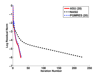
Fig. 1: Log residual-norm plots for the channel-flow Stokes problem with: (A) the standard Uzawa algorithm (8a)–(8b) for $\nu=1$ on the $64\times 64$ grid and (B) the preconditioned Uzawa algorithm (9a)–(9b) for $\nu=1$ on the $32\times 32$ grid.

We now consider the preconditioned Uzawa algorithm (9a)–(9b) applied to this Stokes problem. The preconditioners $Q_{A}$ and $Q_{B}$ are as described in Subsection 4.2, and PGMRES is GMRES applied to (15). The methods of main interest are APU, NAPU, and PGMRES. In order to compare with other splitting preconditioners, we also include results for RDF. As in the unpreconditioned case, convergence of APU is not sensitive to the truncation parameter $m$ in AA. Since convergence is somewhat faster than in the unpreconditioned case, we used $m=10$ in the experiments reported here. We also observed that convergence is not strongly dependent on the relaxation parameter $\omega$ in (9b) in this case, and we used $\omega=1$ in these experiments.

Table 2 shows the number of iterations required by the methods to satisfy (24). As in the unpreconditioned case, acceleration significantly reduced the necessary number of iterations, and again the convergence of all methods appears to be mesh-independent.

Figure 1 (B) shows the log residual-norm plots for the four methods corresponding to the $32\times 32$ grid case in Table 2. The log residual-norm plots for APU, PGMRES, and RDF decrease rapidly. In contrast, the curve for NAPU decreases much more slowly.

Table 2: Iterations required to satisfy (24) for the channel-flow Stokes problem with $\nu=1$. In the RDF column, the numbers in parentheses are the values of ${\beta_{RDF}}$ used in each case.

Grid	APU (10)	NAPU	PGMRES (10)	RDF(10)
$16\times 16$	10	44	10	10 (0.0044)
$32\times 32$	10	43	11	11 (0.0014)
$64\times 64$	11	41	12	11 (0.0003)
$128\times 128$	11	38	12	10 (0.0001)
$256\times 256$	11	36	12	9 (0.0003)

4.4 Lid-driven cavity

The second test problem is the “leaky” lid-driven cavity problem on the square domain $\Omega=[-1,1]\times[-1,1]$. With the “lid” moving from left to right, the top boundary condition is $u=(1,0)^{T}$ at $y=1$, $0\leq x\leq 1$. No-flow boundary conditions $u=(0,0)^{T}$ are imposed on the other three sides. In our experiments, we again discretized the problem on the five uniform grids used in Section 4.3, resulting in the same respective numbers of unknowns. In these and all subsequent experiments reported here, results were obtained using only the preconditioned Uzawa algorithm (9a)$-$(9b).

We first consider the Stokes equations (21)$-$(20) and take $\nu=1$ in (21). In this case, it was sufficient to use $\omega=1$ in (9b), and $m=10$ led to adequately fast convergence of APU. The results for this case are summarized in Table 3. As in the channel-flow problem in Section 4.3, APU(10), PGMRES(10), and RDF(10) performed about the same at all grid sizes in our tests, and all three required significantly fewer iterations to converge than NAPU. Again, the convergence of all methods appears to be mesh-independent.

Table 3: Iterations required to satisfy (24) for the leaky lid-driven cavity Stokes problem with $\nu=1$. In the RDF column, the numbers in parentheses are the values of ${\beta_{RDF}}$ used in each case.

Grid	APU(10)	NAPU	PGMRES(10)	RDF(10)
$16\times 16$	12	49	12	12 (0.004)
$32\times 32$	12	50	14	12 (0.0015)
$64\times 64$	12	50	14	13 (0.0004)
$128\times 128$	11	49	14	13 (0.0001)
$256\times 256$	11	48	14	13 (0.00002)

We next consider the Oseen equations (22)$-$(20) and report results for $\nu=.1$, $.01$, and $.001$. For this more challenging problem, we used $m=20$ in APU in all tests. Also, for $\nu=0.1$ and $\nu=0.01$, we experimentally determined values of $\omega$ in (9b) that approximately minimized the numbers of NAPU iterations. For $\nu=.001$, we were unable to find an $\omega$ for which NAPU converged, and so we determined values of $\omega$ that approximately minimized the numbers of APU iterations (except for the $16\times 16$ grid, for which no method converged for any value of $\omega$). We did not include RDF in these tests since a complete account of its performance on this problem is reported in [10]. The results are summarized in Table 4. In the table, “$>1000$” indicates that the iterates appeared to be converging but failed to satisfy (24) within $1000$ iterations; an asterisk indicates that the iterates did not appear to be converging.

Table 4: Iterations required to satisfy (24) for the leaky lid-driven cavity Oseen problem with $\nu=.1$, $.01$, and $.001$. The values of $\omega$ in (9b) shown in the table were experimentally determined to approximately minimize the numbers of NAPU iterations when $\nu=.1$ and $\nu=.01$ and to approximately minimize the numbers of APU iterations when $\nu=.001$.

	Grid	$\omega$	APU(20)	NAPU	PGMRES(20)
$\nu=.1$	$16\times 16$	0.64	10	11	10
	$32\times 32$	0.45	12	17	12
	$64\times 64$	0.29	15	27	15
	$128\times 128$	0.16	18	46	18
	$256\times 256$	0.087	28	77	41
$\nu=.01$	$16\times 16$	1.2	16	51	16
	$32\times 32$	0.74	21	91	20
	$64\times 64$	0.43	23	148	24
	$128\times 128$	0.24	31	244	40
	$256\times 256$	0.12	32	402	48
$\nu=.001$	$16\times 16$	$*$	$*$	$*$	$*$
	$32\times 32$	1.6	99	$*$	378
	$64\times 64$	0.87	111	$*$	600
	$128\times 128$	0.31	99	$*$	$>1000$
	$256\times 256$	0.17	113	$*$	$>1000$

One sees from Table 4 that, for $\nu=.1$ and $\nu=.01$, acceleration not only significantly reduced iteration numbers but also mitigated mesh dependence, which is at most mild for APU(20) but pronounced for NAPU. Moreover, for $\nu=.001$, acceleration greatly improved robustness, with APU(20) succeeding except on the $16\times 16$ grid while NAPU failed on all grids.

A striking aspect of the results in Table 4 is the difference in performance of APU(20) and PGMRES(20) when the number of iterations is greater than 20. As discussed in Section 3.3, the “essential equivalence” of APU and PGMRES is theoretically assured only when the acceleration in APU is not truncated and PGMRES is not restarted. Evidently, the performance differences seen in Table 4 result from truncating APU and restarting PGMRES, with the latter having more significant negative effects on performance than the former.

To further investigate the effects of the choice of the restart value on PGMRES convergence on this problem, we tried a number of different restart values with $\nu=.001$ on the $64\times 64$ grid. The results are in Table 5. One sees that performance comparable to that of APU(20) in Table 4 was achieved, but only with a restart value much greater than 20 and a correspondingly greater cost of storage and arithmetic.

Table 5: Iterations required by restarted PGMRES to satisfy (24) for the leaky lid-driven cavity Oseen problem with $\nu=.001$ on the $64\times 64$ grid with $\omega=0.87$ (cf. Table 4).

Restart Value	20	30	40	50	60	70
Iterations	600	343	190	167	131	98

We also explored the sensitivity of APU convergence to the parameter $m$, the number of stored residuals in AA. In Fig. 2, we illustrate how the convergence of APU varies with $m$ for the Stokes and Oseen equations. For the Stokes equations, the log residual-norm plots decrease smoothly and show relatively little sensitivity to $m$, with little meaningful difference in the plots for the four values of $m$. For the Oseen equations, the plots decrease smoothly for the most part, although there is a modest plateau region in the middle iterations. There is also somewhat greater sensitivity to $m$ in this more challenging case.

(A)                                            (B)

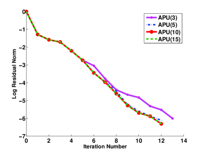
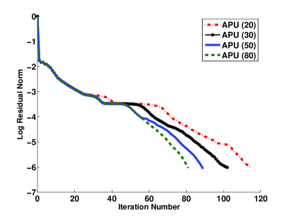
Fig. 2: Log residual norm plots for the leaky lid-driven cavity problem using different numbers of stored residuals $m$ in APU on the $64\times 64$ grid: (A) for the Stokes equations with $\nu=1$ in (21) and $\omega=1$ in (9b) (cf. Table  3); (B) the Oseen equations with $\nu=0.001$ in (21) and $\omega=0.87$ in (9b) (cf. Table 4).

4.5 Flow past an obstacle

The next test problem is flow past an obstacle. This corresponds to channel flow inside the domain $\Omega=[0,8]\times[-1,1]$ with a square object located at $[0,2]\times[0.5,0.5]$. The boundary conditions are as in Subsection 4.3 blackexcept Neumann boundary conditions are set for the outflow. We consider four different grid sizes $16\times 32$, $32\times 64$, $64\times 128$, and $128\times 256$ corresponding to 2488, 9512, 37168, and 146912 unknowns, respectively. We again focus on the preconditioned Uzawa algorithm (9a)$-$(9b) with and without acceleration applied to the Oseen equations (22)$-$(20) and take $m=20$ in APU($m$). We include results for RDF, since to our knowledge these have not been reported elsewhere. For this problem and the backward-facing step problem considered next, the smallest value of $\nu$ considered was $.005$, rather than $.001$, consistent with observations in [10] that a steady solution would be unstable for the latter problem with $\nu=.001$. The results are summarized in Table 6.

Table 6: Iterations required to satisfy (24) for the obstacle-flow Oseen problem with $\nu=.1$, $.01$, and $.005$. The values of $\omega$ in (9b) shown in the table were experimentally determined to approximately minimize the numbers of NAPU iterations for each value of $\nu$. In the RDF column, the numbers in parentheses are the values of ${\beta_{RDF}}$ used in each case.

	Grid	$\omega$	APU(20)	NAPU	PGMRES(20)	RDF(20)
$\nu=.1$	$16\times 32$	0.72	12	13	11	16 (0.044)
	$32\times 64$	0.49	13	17	13	17 (0.014)
	$64\times 128$	0.34	16	25	15	17 (0.005)
	$128\times 256$	0.21	19	39	18	16 (0.001)
$\nu=.01$	$16\times 32$	1.61	34	138	36	18 (0.096)
	$32\times 64$	1.12	25	67	26	20 (0.041)
	$64\times 128$	0.85	16	21	16	22 (0.013)
	$128\times 256$	0.49	14	19	16	24 (0.004)
$\nu=.005$	$16\times 32$	1.28	55	489	66	21 (0.100)
	$32\times 64$	0.76	50	332	57	19 (0.050)
	$64\times 128$	0.76	28	77	30	31 (0.013)
	$128\times 256$	0.52	16	36	16	34 (0.005)

The results in Table 6 show that, as in the previous test problems, acceleration was effective in reducing the number of preconditioned Uzawa iterations. When $\nu=.1$, acceleration also mitigated mesh dependence somewhat, although it is fairly mild for NAPU in this case. Interestingly, when $\nu=.01$ and $\nu=.005$, the iteration numbers required by APU(20), NAPU, and PGMRES(20) all decrease as the grid is refined. For all $\nu$ values, the iteration numbers for APU(20) and PGMRES(20) consistently differ by little, in contrast to the previous problem. The iteration numbers for RDF(20) suggest at most mild mesh dependence for that method. They are about the same as those of APU(20) and PGMRES(20) when $\nu=.1$. For the two smaller values of $\nu$, they are somewhat smaller for the two coarser grids and somewhat larger for the two finer grids.

To further illustrate the convergence of the methods, we show in Fig. 3 (A) the log residual-norm plots of APU(20), NAPU, PGMRES(20), and RDF(20) for the case $\nu=0.01$ and the $32\times 64$ grid. Also, we note that the choice of $m$, the number of stored residuals in AA, does matter for this Oseen problem. In Fig. 3 (B), we show results for different choices of $m$ for this problem with $\nu=0.005$ on the $32\times 64$ grid. The figure clearly indicates that APU($m$) converges faster as $m$ increases. It is also notable that significant improvement over NAPU was obtained with $m$ as small as five.

(A)                                            (B)

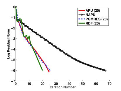
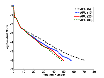
Fig. 3: Log residual-norm plots for the obstacle-flow Oseen problem on the $32\times 64$ grid: (A) all methods with $\nu=.01$; (B) APU($m$) for different $m$ with $\nu=.005$ (cf. Table 6).

4.6 Backward-facing step

Our final test problem is flow over a backward-facing step. In this, the domain is $\Omega=[-1,0]\times[0,1]\cup[0,5]\times[-1,1]$, which has a downward “step” at $x=0$. As in Subsection 4.3, a parabolic flow profile is imposed at the inflow boundary ($x=-1$ and $0\leq y\leq 1$). Neumann boundary conditions are imposed at the outflow boundary ($x=5$ and $-1<y<1$). At the other walls, a no-flow boundary is prescribed. We study the problem using four different grids having the general form $2^{n}\times 3\cdot 2^{n}$ for $n=4,5,6,7$, corresponding to 1747, 6659, 25987, and 102659 unknowns, respectively. As in Subsection 4.5, we consider the Oseen equations (22)$-$(20) with $\nu=.1$, $\nu=.01$, and $\nu=.005$ and report on the performance of the methods with $m=20$ in APU($m$). The results are summarized in Table 7.

Table 7: Iterations required to satisfy (24) for the backward-facing step Oseen problem with $\nu=.1$, $.01$, and $.005$. The values of $\omega$ in (9b) shown in the table were experimentally determined to approximately minimize the numbers of NAPU iterations for each value of $\nu$. In the RDF column, the numbers in parentheses are the values of ${\beta_{RDF}}$ used in each case.

	Grid	$\omega$	APU(20)	NAPU	PGMRES(20)	RDF(20)
$\nu=.1$	$16\times 48$	0.64	11	12	11	15 (0.035)
	$32\times 96$	0.45	14	17	14	14 (0.014)
	$64\times 192$	0.29	17	26	17	13 (0.005)
	$128\times 384$	0.17	20	40	19	14 (0.0009)
$\nu=.01$	$16\times 48$	0.93	24	61	24	15 (0.140)
	$32\times 96$	0.55	15	25	14	15 (0.043)
	$64\times 192$	0.46	14	24	14	16 (0.013)
	$128\times 384$	0.38	19	32	20	17 (0.005)
$\nu=.005$	$16\times 48$	0.44	41	400	40	20 (0.170)
	$32\times 96$	0.42	28	112	31	19 (0.061)
	$64\times 192$	0.32	20	49	20	19 (0.017)
	$128\times 384$	0.31	21	36	20	19 (0.006)

The results in Table 7 are qualitatively very similar to those in Table 6. As in that case, acceleration was effective in reducing the number of preconditioned Uzawa iterations and also in mitigating the rather mild mesh dependence of NAPU when $\nu=.1$. When $\nu=.01$ and $\nu=.005$, the table shows some tendency for the iteration numbers of APU(20), NAPU, and PGMRES(20) to actually decrease as the grid is refined, although it is not as pronounced or consistent as in the previous case. The iteration numbers for APU(20) and PGMRES(20) are very similar and do not differ much from those of RDF(20), which show no significant mesh dependence. We note that this problem is considered in [8] but only for $\nu=.005$ on the $16\times 48$, $32\times 96$, and $64\times 192$ grids. In these cases, the results for RDF(20) shown here are slightly more favorable than those in [8], presumably because of slightly different values of ${\beta_{RDF}}$ (denoted by $\alpha$ in [8]). We conclude this section by showing in Figure 4 the performance of all methods in the case of $\nu=.005$ and the $32\times 96$ grid.

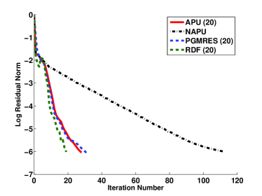
Fig. 4: Log residual-norm plots for all methods on the backward-facing step Oseen problem with viscosity $\nu=0.005$ and the $32\times 96$ grid (cf. Table 7).

5 Discussion & Conclusions

We have introduced Anderson acceleration (AA) as an easily implemented and economical way of improving the convergence of the Uzawa algorithm for solving a saddle-point system (7). While such systems arise in many settings, the applications of primary interest here are the steady Stokes and Oseen problems of incompressible flow. As far as we know, this is the first time that AA has been used either with the Uzawa algorithm in any context or with any iterative method for these Stokes and Oseen problems.

After introducing the standard (unpreconditioned) and preconditioned Uzawa algorithms in Section 2, we describe AA in Section 3 and discuss its application to the Uzawa algorithm. We show that, viewed as a fixed-point iteration, the preconditioned Uzawa algorithm is a stationary iteration for (7) determined by the splitting (13). It follows from results in [40] that preconditioned Uzawa accelerated with untruncated AA is “essentially equivalent” in a certain sense to unrestarted GMRES applied to the preconditioned system (14). When the Uzawa preconditioning matrix $Q_{A}$ in (9a) is equal to $A$, the preconditioned system (14) simplifies to (15), a form especially convenient for applying GMRES. Similar results hold for standard Uzawa as a special case, with the simplified form of the preconditioned system given by (16).

In Section 4, we present results of extensive numerical experiments comparing the performance of the Uzawa algorithm with and without acceleration in several steady Stokes and Oseen incompressible-flow scenarios. Our main interest is in the preconditioned Uzawa algorithm (9a)$-$ (9b), with preconditioning as described in Section 4.2; however, we also report results for the unpreconditioned algorithm (8a)$-$(8b) in one case, the channel-flow Stokes problem considered in Section 4.3. In discussing the test results below, we often refer to methods using the acronyms given in Section 4.2; for example, PGMRES refers to GMRES applied to the preconditioned system (15).

Although, as noted above, unrestarted PGMRES is “essentially equivalent” to Uzawa accelerated with untruncated AA, this equivalence does not hold when PGMRES is restarted and AA is truncated. Consequently, we included restarted PGMRES in our tests in order to see how its performance compared to that of Uzawa accelerated with truncated AA. To broaden the comparison, we also included in most test cases GMRES applied to the equivalent system (18) preconditioned with the sophisticated Relaxed Dimensional Factorization preconditioner developed in [10], referred to simply as RDF here.

In all test cases, acceleration reduced the numbers of iterations required by the Uzawa algorithm to satisfy the convergence criterion (24). The reduction was usually significant, and in many cases it was dramatic. Accelerated Uzawa usually required about the same numbers of iterations or modestly fewer than restarted PGMRES; however, in one case, that of the leaky lid-driven cavity problem (see Table 4), the accelerated method APU(20) was significantly more robust than PGMRES(20) and often required significantly fewer iterations when the iterates from both methods converged. The results in Table 5 suggest that the PGMRES iterates can be made to converge in as few iterations as those of APU(20) in this test case, but only by taking the restart value to be much larger than 20.

Accelerated Uzawa usually required about the same numbers of iterations as RDF, although not in every case (see, e.g., Table 6). We note that the RDF preconditioner $M_{\beta}$ in (18) depends on a parameter $\beta$. Although some guidelines for choosing $\beta$ are given in [10], determining effective values of $\beta$ may require some effort in practice. In our tests, values of $\beta$ were determined through auxiliary experimentation to give near-optimal convergence in each case.

We also used auxiliary experimentation to determine values of the parameter $\omega$ in the standard and preconditioned Uzawa iterations (8a)$-$(8b) and (9a)$-$(9b) that approximately minimized the numbers of non-accelerated Uzawa iterations in each test case. Developing more efficient methods for determining effective choices of $\beta$ in (18) and $\omega$ in the Uzawa iteration will be a subject of future work.

In the tests involving Stokes flow (see Tables 1-3), all methods showed little adverse mesh dependence. This is not surprising, in view of the mesh-independence property of non-accelerated Uzawa for Stokes flow noted in [8, §8.1]. In the tests with Oseen flow (see Tables 4-7)), the RDF method showed at most very modest mesh dependence in all cases. With the other methods, mesh dependence varied considerably. For the leaky lid-driven cavity Oseen problem (Table 4), mesh dependence of the non-accelerated preconditioned Uzawa algorithm NAPU was pronounced, while that of the accelerated method APU(20) was much more benign. For the obstacle-flow and backward-facing step Oseen problems (Tables 6 and 7), convergence of both NAPU and APU(20) was not very adversely affected and, in some cases, actually improved as the mesh was refined.

There are other Uzawa-like methods for iteratively solving the saddle-point system (7) that we have not considered here. For instance, if $Q_{A}^{-1}$ in (2.2a) is replaced by $Q_{A}^{-1}=\eta P^{-1}$, where $\eta$ is a positive relaxation parameter and $P$ is a preconditioner, then the system (9a)–(9b) is called the parameterized inexact Uzawa (PIU) method [5]. Several frameworks have been developed for the PIU method to accelerate convergence to solutions for both the symmetric and nonsymmetric generalized saddle-point problems [6]. Another class of PIU methods has been developed recently to iteratively solve for solutions of complex symmetric linear systems [44]; these methods accelerate convergence using a correction technique. The corrected PIU methods are also shown to have faster convergence compared to some Uzawa-type and Hermitian or skew-Hermitian splitting-type methods [44]. Other Uzawa-like methods have been proposed in recent years to solve saddle-point systems. These methods include Uzawa-SOR, Uzawa-AOR, Uzawa-SAOR, and Uzawa-SSOR [43, 42]. These methods utilize the decomposition of the matrix $A$ as $A=D-L-U$, where $D,L,$ and $U$ are diagonal, strictly lower-triangular, and strictly upper-triangular, respectively. The proposed methods are effective in solving the saddle-point system and have less computational time compared to the generalized SOR method [43].

While we have focused on fluid flow governed by the Stokes and Oseen equations, Uzawa-like methods have also been applied to other fluid models, including non-Newtonian fluids such as viscoplastic and viscoelastic fluids. For instance, a convergence study and numerical simulations for the Bingham model of a viscoplastic fluid has been investigated in [18]. Simulations for unsteady Bingham flow in cylinders and in a lid-driven cavity using the Newton-Conjugate Gradient-Uzawa algorithm were studied where the problems were discretized using finite-element methods [18]. For viscoelastic fluids, a time-dependent Oldroyd model has been treated using an Uzawa-like scheme called the gauge-Uzawa (projection-Uzawa) finite-element method [39]. In this method, the velocity component is decomposed into an unknown vector and an auxiliary scalar variable, easily handling boundary derivatives. This method, however, does not require the formation of the saddle-point system. In the future, we will explore extending the accelerated Uzawa schemes to solve non-Newtonian fluid problems.

References

- [1] D. G. Anderson, Iterative procedures for nonlinear integral equations, J Assoc Comput Machinery, 12 (1965), pp. 547–560.
- [2] K. J. Arrow, L. Hurwicz, and H. Uzawa, Studies in Linear and Nonlinear Programming, Stanford University Press, Stanford, CA, 1958.
- [3] C. Bacuta, B. McCracken, and L. Shu, Residual reduction algorithms for nonsymmetric saddle point problems, J Comput Appl Math, 235 (2011), pp. 1614–1628.
- [4] Z.-Z. Bai, G. H. Golub, and M. K. Ng, Hermitian and skew-Hermitian splitting methods for non-Hermitian positive definite linear systems, SIAM J Matrix Anal Appl, 24 (2003), pp. 603–626.
- [5] Z.-Z. Bai, B. N. Parlett, and Z.-Q. Wang, On generalized successive overrelaxation methods for augmented linear systems, Numer Math, 102 (2005), pp. 1–38.
- [6] Z.-Z. Bai and Z.-Q. Wang, On parameterized inexact Uzawa methods for generalized saddle point problems, Linear Algebra and Appl, 428 (2008), pp. 2900–2932.
- [7] M. Benzi, A generalization of the Hermitian and skew-Hermitian splitting iteration, SIAM J Matrix Anal Appl, 31 (2009), pp. 360–374.
- [8] M. Benzi, G. H. Golub, and J. Liesen, Numerical solution of saddle point problems, Acta Numerica, 2005 (2005), pp. 1–137.
- [9] M. Benzi and X. P. Guo, A dimensional split preconditioner for Stokes and linearized Navier–Stokes equations, Appl Numer Math, 61 (2011), pp. 66–76.
- [10] M. Benzi, M. Ng, Q. Niu, and Z. Wang, A relaxed dimensional factorization preconditioner for the incompressible Navier–Stokes equations, J Comput Phys, 230 (2011), pp. 6185–6202.
- [11] M. Benzi, M. A. Olshanskii, and Z. Wang, Modified augmented Lagrangian preconditioners for the incompressible Navier–Stokes equations, Int J Num Methods Fluids, 66 (2010), pp. 486–508.
- [12] J. H. Bramble, J. E. Pasciak, and A. T. Vassilev, Analysis of the inexact Uzawa algorithm for saddle point problems, SIAM J Numer Anal, 34 (1997), pp. 1072–1092.
- [13] , Uzawa type algorithms for nonsymmetric saddle point problems, Math Comput, 69 (1999), pp. 667–689.
- [14] M. T. Calef, E. D. Fichtl, J. S. Warsa, M. Berndt, and N. N. Carlson, Nonlinear Krylov acceleration applied to a discrete ordinates formulation of the k-eigenvalue problem, J Comput Phys, 238 (2013), pp. 188–209.
- [15] Z. H. Cao, Fast Uzawa algorithm for generalized saddle point problems, Appl Num Math, 46 (2003), pp. 157–171.
- [16] C. Chen and C. Ma, A generalized shift-splitting preconditioner for saddle point problems, Appl Math Lett, 43 (2015), pp. 49–55.
- [17] M. R. Cui, Analysis of iterative algorithms of Uzawa type for saddle point problems, Appl Num Math, 50 (2004), pp. 133–146.
- [18] E. J. Dean, R. Glowinski, and G. Guidoboni, On the numerical simulation of Bingham visco-plastic flow: old and new results, J Non-Newtonian Fluid Mech, 142 (2007), pp. 36–62.
- [19] H. Elman, V. E. Howle, J. Shadid, D. Silvester, and R. Tuminaro, Least squares preconditioners for stabilized discretizations of the Navier-Stokes equations, SIAM J Sci Comput, 30 (2007), pp. 290–311.
- [20] H. C. Elman, Multigrid and Krylov subspace methods for the discrete Stokes equations, Int J Num Methods Fluids, 22 (1996), pp. 755–770.
- [21] H. C. Elman and G. H. Golub, Inexact and preconditioned Uzawa algorithms for saddle point problems, SIAM J Numer Anal, 31 (1994), pp. 1645–16661.
- [22] H. C. Elman, V. E. Howle, J. Shadid, R. Shuttleworth, and R. Tuminaro, Block preconditioners based on approximate commutators, SIAM J Sci Comput, 27 (2006), pp. 1651–1668.
- [23] H. C. Elman, A. Ramage, and D. J. Silvester, IFISS: A Matlab toolbox for modelling incompressible flow, ACM Trans Math Software, 33 (2007), p. 14.
- [24] H. C. Elman, D. J. Silvester, and A. J. Wathen, Finite elements and fast iterative solvers: with applications in incompressible fluid dynamics, Oxford University Press, 2014.
- [25] H. Fang and Y. Saad, Two classes of multisecant methods for nonlinear acceleration, Numer Linear Algebra Appl, 16 (2009), pp. 197–221.
- [26] V. Ganine, N. J. Hills, and B. L. Lapworth, Nonlinear acceleration of coupled fluid-structure transient thermal problems by Anderson mixing, Int J Num Methods Fluids, 71 (2013), pp. 939–959.
- [27] R. Glowinski, Numerical Methods for nonlinear variational problems, Springer series in Computational Physics, Springer, NY, 1984.
- [28] Q. Y. Hu and J. Zou, Nonlinear inexact Uzawa algorithms for linear and nonlinear saddle-point problems, SIAM J Optim, 16 (2006), pp. 798–825.
- [29] A. Klawonn, An optimal preconditioner for a class of saddle point problems with a penalty term, SIAM J Sci Comput, 19 (1998), pp. 540–552.
- [30] D. Kuzmin, Linearity-preserving flux correction and convergence acceleration for constrained Galerkin schemes, J Comput Appl Math, 236 (2012), pp. 2317–2337.
- [31] Y. Lin and Y. Cao, A new nonlinear Uzawa algorithm for generalized saddle point problems, Appl Math Comput, 75 (2006).
- [32] K. Lipnikov, D. Svyatskiy, and Y. Vassilevski, Anderson acceleration for nonlinear finite volume scheme for advection-diffusion problems, SIAM J Sci Comput, 35 (2013), pp. A1120–A1136.
- [33] W. Liu and S. Xu, An new improved Uzawa method for finite element solution of Stokes problem, Comput Mechanics, 27 (2001), pp. 305–310.
- [34] P. A. Lott, H. F. Walker, C. S. Woodward, and U. M. Yang, An accelerated Picard method for nonlinear systems related to variably saturated flow, Advances in Water Resources, 38 (2012), pp. 92–101.
- [35] A. Quarteroni and A. Valli, Numerical Approximation of Partial Differential Equations, Springer-Verlag, Berlin Heidelberg, 1994.
- [36] W. Queck, The convergence factor of preconditioned algorithms of the Arrow-Hurwicz type, SIAM J Num Anal, 26 (1989).
- [37] Y. Saad and M. H. Schultz, GMRES: a generalized minimal residual method for solving nonsymmetric linear systems, SIAM J Sci Stat Comput, 7 (1986), pp. 856–869.
- [38] D. K. Salkuyeh, M. Masoudi, and D. Hezari, On the generalized shift-splitting preconditioner for saddle point problems, Appl Math Lett, 48 (2015), pp. 55–61.
- [39] Z. Si, W. Li, and Y. Wang, A gauge-Uzawa finite element method for the time-dependent Viscoelastic Oldroyd flows, J Math Anal and Appl, 425 (2015), pp. 96–110.
- [40] H. F. Walker and P. Ni, Anderson acceleration for fixed-point iterations, SIAM J Numer Anal, 49 (2011), pp. 1715–1735.
- [41] M. H. Wright, Interior methods for constrained optimization, Acta Numerica, 1 (1992), pp. 341–407.
- [42] J. H. Yun, Variants of the uzawa method for saddle point problem, Comput Math Appl, 65 (2013), pp. 1037–1046.
- [43] J. Zhang and J. Shang, A class of Uzawa-SOR methods for saddle point problems, Appl Math Comput, 216 (2010), pp. 2163–2168.
- [44] Q.-Q. Zheng and C.-F. Ma, Fast parameterized inexact Uzawa method for complex symmetric linear systems, Appl Math Comput, 256 (2015), pp. 11–19.
- [45] W. Zulehner, Analysis of iterative methods for saddle point problems: a unified approach, Math Comput, 71 (2001), pp. 479–505.