MODELING RESPONSE TIME WITH POWER-LAW DISTRIBUTIONS

Abstract

Understanding the properties of response time distributions is a long-standing problem in cognitive science. We provide a tutorial overview of several contemporary models that assume power law scaling is a plausible description of the skewed heavy tails that are typically expressed in response time distributions. We discuss several properties and markers of these distribution functions that have implications for cognitive and neurophysiological organization supporting a given cognitive activity. We illustrate how a power law assumption suggests that collecting larger samples, and combining individual subjects’ data into a single set for a distribution-function analysis allows for a better comparison of a group of interest to a control group. We demonstrate our techniques in contrasts of response time measurements of children with and without dyslexia.

1 Introduction

Response time (RT) is the elapsed interval between the presentation of a stimulus and the execution of a response in a laboratory-based cognitive task. Response times are widely used in basic cognitive science and are also routinely used in neuropsychiatric assessments for certain cognitive impairments and reading disabilities (e.g. Ancelin et al., 2006; Epstein et al., 2011; Tse et al., 2010). To date, there is little scientific consensus regarding the fundamental statistical properties of response time distributions themselves. In light of their widespread use, an accurate statistical description of response time distributions would be extremely useful.

The focus of this article is response time probability density functions (PDFs) that include skewed power-law tails. We tentatively assume that response time PDFs are at least approximately stationary – they stabilize near a steady state for a given cognitive activity. This assumption is tentative because recent reports established that time-series of response times express $1/f$ noise – long-range correlations and fractional dimensionality (Van Orden et al., 2003, 2005). Moreover, several groups have proposed that the characteristic positive skew in tails of response time distributions conforms to a power-law function (Holden & Rajaraman, 2012; Ihlen, 2013).

Previously, we examined the skewed tails of the probability distribution function of response times (Holden & Rajaraman, 2012; Holden et al., 2009; Ma et al., 2015). Power-law scaling prevailed as a more plausible description of empirical distribution’s tail behavior than models that adopted exponentially decaying tail behavior or even heavy-tailed lognormal behavior. In what follows, we first introduce three candidate distributions that implement power-law tails: The L$\acute{e}$vy alpha-stable distribution (S), the generalized inverse gamma distribution (GIGa) and the ”Cocktail” lognormal/Pareto (LNP) mixture distribution. Following our introduction to the power-law distribution models, we use both the GIGa and the LNP distributions to introduce heavy-tailed research design practices and other methods for aggregating response time observations for the purpose of statistical inference. Finally, we illustrate the use of these selected techniques on a published data set that contrasted a sample of dyslexic and matched age-appropriate readers.

2 Potential Model Distributions with Power-law Tails

Here we summarize the properties of the potential model distributions with power-law tails. More detailed explanations of the role of the scale, shape, and location parameters appear in Sec. 4 in the context of the discussion of distribution rescaling.

2.1 The Stable Distribution

With the exception of $\alpha=2$, when it reduces to normal distribution (N), the S distribution (Nolan, 2015), has a power-law tail

$$S(x;\alpha,\beta,\mu,\sigma)\sim|x|^{-(1+\alpha)}$$ (1)

Here stability $0<\alpha<2$ , defined below, and skewness $-1\leq\beta\leq 1$ are the shape parameters of the distribution, while $\sigma$ and $\mu$ are its scale and location parameters. In general, S does not have a closed-form expression – among notable exceptions are the Cauchy and L$\acute{e}$vy distributions – instead, it is described by a closed-form characteristic function and via parametric forms.

The two important properties of S are as follows. First, the sum of two independent identical variables (iid) distributed with $S(x;∗,∗,∗,\sigma)$, is distributed with $S(x;∗,∗,∗,2^{1/\alpha}\sigma)$. That is, the linear combination of iid’s results in the same distribution, up to a rescaled scale parameter – this is the definition of stability. Second, the sum of independent identically distributed variables, whose PDF has an $|x|^{-(1+\alpha)}$ tail, $0<\alpha<2$, tends to $S(x;\alpha,0,0,\sigma)$ as the number of variables in the sum grows, by the Generalized Central Limit Theorem. These properties account for the so called ”Noah Effect” and resulting $H=1/\alpha\neq 1/2$ Hurst exponent (Mandelbrot, 2002). Note, however, while $H=1/2$ for $\alpha>2$, according to CLT, the number of variables in the sum and the corrections to N are abnormally large for fat tails (Lam et al., 2011).

Ihlen (2013), proposed S for fitting of RT distributions. While an attractive proposition due to its properties above – namely, power-law tails and additivity – the two main drawbacks are that the power-tail exponents, $(1+\alpha)$, are limited to the $(1,3)$ range and that the only allowed value of $\beta$ is $\beta=1$, since otherwise the variable of the distribution is not positively defined, as is physically meaningful for RT. The allowed values of the exponent, however, contradict the observed exponent values of several RT studies (see, for instance, (Holden & Rajaraman, 2012; Ma et al., 2015)).

2.2 Generalized Inverse Gamma Distribution

The application of GIGa to RT distribution fitting is motivated by its origins in the generalized Bouchaud-M$\acute{e}$zard network model (Bouchaud & Mézard, 2000) – and its implications for brain dynamics – and a related stochastic differential equation describing a stochastic ”birth-death” model (Ma et al., 2015, 2013; Ma & Serota, 2014). GIGa is zero for $x<\mu$, while for $x>\mu$ it is given by

$$GIGa(x;\alpha,\beta,\gamma,\mu)=\frac{\exp\left(-\left(\frac{\beta}{x-\mu}\right)^{\gamma}\right)\gamma\left(\frac{\beta}{x-\mu}\right)^{\alpha\gamma+1}}{\beta\Gamma(\alpha)}$$ (2)

Above, $\alpha$ and $\gamma$ are the shape parameters, $\beta$ is the scale parameter, $\mu$ is the location parameter and $\Gamma$ is the Gamma function. Except for $\mu$, all parameters are positively defined and, in the context of RT, $\mu$ must be non-negative as well. For large $x$, it exhibits power-law tail

$$GIGa(x;\alpha,\beta,\gamma,\mu)\sim x^{-(1+\alpha\gamma)}$$ (3)

Unlike S, there is no a priori upper bound on the tail exponent of GIGa.

2.3 Lognormal/Pareto Mixture Distribution

In the cocktail model (Holden & Rajaraman, 2012; Holden et al., 2009), the LNP mixture distribution is given by

$$\begin{array}[]{rl}LNP(x;\mu,\sigma,\alpha,\rho_{P})=&\begin{array}[]{ccl}\frac{\rho_{<}}{C\sqrt{2\pi}\sigma x}e^{-\frac{(\ln x-\mu)^{2}}{2\sigma^{2}}}&,&x\leq x_{P}\\ \frac{\rho_{>}}{(1-C)\sqrt{2\pi}\sigma x}e^{-\frac{(\ln x-\mu)^{2}}{2\sigma^{2}}}+\frac{\rho_{P}\alpha x_{P}^{\alpha}}{x^{\alpha+1}}&,&x\geq x_{P}\\ \end{array}\end{array}$$ (4)

Here $C=\frac{1}{2}\left(1+Erf\left(\frac{\alpha\sigma}{\sqrt{2}}\right)\right)$, $\alpha$, $\sigma$ and $\rho_{P}$ are the shape parameters and $x_{P}$ is the scale parameter. The other three parameters, $\rho_{<}$, $\rho_{>}$ and $\mu$ are determined from the condition of normalizability of LNP ($\rho_{<}+\rho_{>}+\rho_{P}=1$) and continuity of LNP and its derivative at $x_{P}$ ; in particular, $\mu$ and $x_{P}$ are related by $x_{P}=\exp(\mu+\alpha\sigma^{2})$.

As mentioned before, the choice of LN front end is motivated by multiplicativity. For large $x$,

$$LNP(x;\mu,\sigma,\alpha,\rho_{P})\sim x^{-(1+\alpha)}$$ (5)

As is for GIGa, LNP does not have an upper bound for the tail exponent. However, unlike S and GIGa, which are infinitely differentiable at all points, LNP’s derivatives above first are discontinuous at $x_{P}$.

3 Heavy-Tailed Research Design and Statistics

Systems that express power-law behavior must be studied with methods that accommodate more time-dependence and inherent variability than is typically assumed by linear statistics. The theorems that dictate classical statistical practices are often stretched to, or beyond, their limits in heavy-tailed applications. For example, $1/f$ scaling undermines the classical ergodicity assumption, and much larger sample sizes are required for inference in the context of heavy-tailed systems than those expressing Gaussian behavior. Extreme observations are so rare in Gaussian systems that few experiments are designed to discover them, and unusual observations are reasonably treated as outliers. However, extreme observations are much more likely in systems that express power-law behavior – but they may still be rare. As such it is important to incorporate designs that accommodate much larger samples than is typical under the assumption of linearity.

Whenever possible, within-subject designs are recommended. If two categories of behavior are to be contrasted, pairwise yoking of stimuli often yields a design that is very sensitive for simple distribution contrasts. Each participant is exposed to yoked target stimuli that are matched on important control variables, but that differ in terms of the variable of interest. Both contrast distributions can then be comprised of measurements that originate from the same individuals, on carefully paired target items that differ only in terms of the variable of interest.

However, many experimental manipulations require between-participants’ designs. In decision studies, for instance, one can use an ideal strategy manipulation (Stone & Van Orden, 1993). This design presents identical positive items but allows one to vary categories of distractor catch trials. Apparently, the method originated in lexical decision studies of word recognition, but it could be adapted to other decision paradigms. This design yields contrast distributions that are comprised of responses to identical target items from different individuals who completed conditions with different distractor items. The basic idea behind the manipulation is to use different classes of distractor items that impact the relative difficulty of the required decision or discrimination (e.g., the signal-to-noise ratio).

If enough targets can be presented, both the within and between subjects designs allow one to complete statistical contrasts at the level of both individual participants and analyses that aggregate across participants. In general, aggregated analyses are more powerful, and likely more representative of systems that express rare events. Usually one looks for similar outcomes in aggregated analyses and individual level analyses.

Similarly, some studies are designed to contrast separate groups of individuals, such as clinical classification studies, where a group of interest is compared to the control group. In these studies health impairments may hamper efforts to present enough trials to individuals to yield stable individual level analyses. Given these circumstances, aggregated analyses become more important. Rather than fitting each subject individually, and then averaging the fitting and other parameters over the group, it is often more expedient to aggregate observations from each participant into an omnibus distribution that is fit parametrically. There is a legitimate historical concern in the response time literature that individual and aggregate analyses have the potential to yield qualitatively different outcomes. While discrepant results are certainly possible, we now present simulation studies that test the congruence and validity of individual and aggregate fitting for the power-law models discussed earlier.

We speculate that response time distributions, with particular parameters, observed in the context of a particular cognitive activity, requires the support of a network of particular perceptual, cognitive and neurophysiological process (Holden & Rajaraman, 2012; Holden et al., 2013, 2014). At any given point in time, fluctuations may arise in the organization of this network and its parametric quantities. This is true both within a task and across group contrasts of interest. Under the assumption that we are dealing with a network of processes that express heavy-tailed behavioral measures, individual participant’s performances can be viewed as samples or realizations of random variables that are representative of the potential states of the process network supporting the cognitive activity of interest. Given this situation, combining observations across participants may clarify the potential range of parametric variation that one must expect from a given group or task, and thus improve the representativeness of any statistical analyses that are derived from the distribution of observations. Due to the aforementioned convergence issues, this is especially important for power-law-tail distributions. Conversely, one expects a far greater parameter variation in subject’s power-law-tail distributions, especially for small sample sizes.

To contrast the behavior of individual and aggregated parameter estimates we present the following numerical simulation using GIGa as a candidate distribution:

1. We fit the aggregated RT trials data of each of the two groups with GIGa to obtain the initial values of its parameters $\alpha_{0}^{i}$, $\beta_{0}^{i}$, $\gamma_{0}^{i}$, $\mu_{0}^{i}$, where $i=1,2$ is for control and dyslexic group respectively (for instance, the values in Table 1 are the result of such fits).

2. We use parameters $\alpha_{0}^{i}$, $\beta_{0}^{i}$, $\gamma_{0}^{i}$, $\mu_{0}^{i}$, obtained in step (1), to generate the group-size variates. These variate ”groups” are meant to serve as simulated counterparts of the RT trials control (C) and dyslexic (D) groups used in step (1).

3. We use the bootstrap procedure (Efron & Tibshirani, 1994) on the group variates from step (2) to obtain the bootstrap distribution, mean, standard deviation (SD) and confidence interval (CI) for the parameters $\alpha^{i}$, $\beta^{i}$, $\gamma^{i}$, $\mu^{i}$ of the group variates. There are other ways to generate the variability of parameters – we chose to use bootstrap in order to parallel the procedure of Sec. 5 on RT trials group data.

4. We then generate random variates of the individual-subject size, where the parameters of the candidate distribution are taken at random from a normal distribution, whose mean is the real data parameter from step (1) and SD is obtained in step (3), mimicking the variability of the parameters mentioned above. These subject-size distributions – variate ”subjects” – are individually fitted and we obtain the mean, SD and range of the parameters of these.

5. We then compare the variate ”groups” and variate ”subjects” to the actual RT trials data groups and subjects.

As mentioned above, there are alternative methods of generating parameter variability, described in step (3). For instance, one could resample the raw data distributions or use the Jackknife procedure (Efron & Tibshirani, 1994). In this regard, it should be noted that the bootstrap distributions of parameters of simulated variates are narrower than those of RT trials data, as seen in Figures 1 and 2 (see below). The main conclusion, however, is that a distribution of parameters of aggregated variates are narrower than those derived from individual’s data, be it the RT trials data or their simulated counterparts. This illustrates a potential benefit of aggregation of individual observations. This could be particularly useful when individual observations exert undue influence on parameter estimates, as when sample sizes are small.

Here we implement this approach for the Arithmetic study that contrasted children with and without dyslexia (see Sec. 4 below and (Holden et al., 2014)). Participants pressed one button to indicate that displayed simple addition sums, together with an answer, were correct (e.g., $3+6=9$) and another button if incorrect (e.g., $4+3=2$). The answers to all the sums were always below $10$.

Using GIGa as a candidate distribution, $20$ variate ”Psudo-subjects” of $560$ points each were generated, per steps (1)-(4) above, similar to the actual trials. As an example, we use two measures of variability – the tail exponent is computed from the GIGa parameters as $(\alpha\gamma+1)$ in Eq. (3) and the half width (HW) of the distribution, defined as the width of the distribution along the line drawn at half height of the PDF’s maximum, that is, modal value of PDF (MPDF) – see Sec. 5 below – both of which depend on the shape parameters. The results are summarized in Figures 1 and 2 and Tables 1–4, where ”C” stands for control and ”D” for dyslexic.

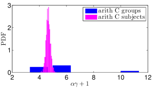
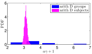
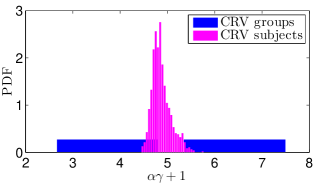
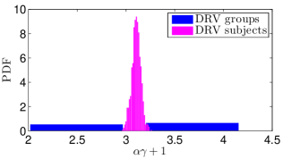
Figure 1: Tail exponent ($\alpha\gamma+1$). Top row: Histograms of parameters derived from fits of individual subjects (blue bars) and from fits of group (aggregate) data (magenta bars), obtained in RT trials for the control and dyslexic groups respectively. Bottom row: Histograms of parameters derived from fits of variate ”subjects” and variate ”groups” – counterparts of the individual and group RT data – obtained in steps (3) and (4) of the random variate simulation described in text.

Tables 1 and 3 contain the results for actual trials data and the statistics for the combined group data are calculated using the bootstrap. In Tables 2 and 4, CRV and DRV are control group and dyslexic group variates respectively; mean, SD and CI for the variate ”groups” are obtained in step (3); mean, SD and range for the variate ”subjects” are obtained in step (4). CI in Tables 1-4 are set to the $95\%$ confidence level.

Table 1: Tail Exponent $\alpha\gamma+1$

	Actual Group				Actual Subjects
	mean	SD	CI		mean	SD	Range
C	4.656	0.161	(4.469,	5.114)	5.383	2.240	(3.140,	11.511)
D	3.112	0.087	(2.948,	3.291)	3.801	1.241	(2.102,	6.879)

Table 2: Variate Tail Exponent $\alpha\gamma+1$

	”Pseudo-Group” Variate				”Pseudo-Subjects” Variate
	mean	SD	CI		mean	SD	Range
CRV	4.868	0.198	(4.479,	5.135)	4.941	1.560	(2.398,	7.760)
DRV	3.106	0.046	(3.055,	3.235)	3.130	0.712	(1.901,	4.272)

Comparing the dispersion of the synthetic individual fits to that of the all-in-one fits recommends an all-in-one approach. Given the potential noisiness of performance data from children, and that each group, control and dyslexic, contribute only about $10^{4}$ combined data points, the quantitative agreement seems to be quite good as well.

Likewise, contrasts of the confidence intervals for the synthetic group variables and actual group data with the ranges for subjects’, demonstrates that fitting of individual subjects, with subsequently averaged parameters, may be not sufficiently accurate to distinguish rescaled distributions (see Sec. 4 and 5) from those of different shape and, by proxy, distinct underlying relations among cognitive and neurophysiological processes.

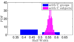
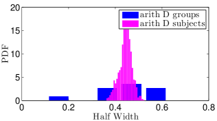
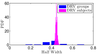
Figure 2: Half Width histograms. Top row: Histograms of parameters derived from fits of individual subjects (blue bars) and from fits of group (aggregate) data (magenta bars), obtained in RT trials for the control and dyslexic groups respectively. Bottom row: Histograms of parameters derived from fits of variate ”pseudo-subjects” and variate ”pseudo-groups” – counterparts of the individual and group RT data – obtained in steps (3) and (4) of the random variate simulation described in text.

Table 3: Half-Width (HW)

	Actual Group				Actual Subjects
	mean	SD	CI		mean	SD	Range
C	0.559	0.015	(0.543,	0.599)	0.463	0.087	(0.364,	0.634)
D	0.444	0.026	(0.380,	0.487)	0.447	0.140	(0.106,	0.626)

Table 4: Variate Half-Width (HW)

	”Pseudo-Group” Variate				”Pseudo-Subjects” Variate
	mean	SD	CI		mean	SD	Range
CRV	0.572	0.007	(0.559,	0.587)	0.515	0.079	(0.302,	0.600)
DRV	0.447	0.009	(0.433,	0.469)	0.405	0.112	(0.142,	0.720)

Next, we discuss several interpretable differences that can appear in the parameters of heavy-tailed distributions arising from systems that are governed by interaction-dominant dynamics (Holden et al., 2009; Van Rooij et al., 2013). Finally, we illustrate the technique on data from a recently published dyslexia study (Holden et al., 2014).

4 Rescaling

Suppose one collects RT data, in an identical experimental setup, from two distinct groups of participants – for instance, children with and without dyslexia. Is it possible to relate the underlying relationships among cognitive and neurophysiological systems to the shape of the response time PDF? If the aggregate distributions of the two groups happen to be the rescaled versions of each other, we posit that the supporting networks of perceptual, cognitive and neurophysiology processes is functioning in a qualitatively similar manner, as the only difference entailed in rescaling is time dilation or time contraction. By contrast, substantial shape differences imply the functional organization of the supporting perceptual, cognitive and neurophysiological systems is different. So if

$$PDF_{2}(c\cdot x)=\frac{1}{c}PDF_{1}(x)$$ (6)

where

$$c=\frac{mean_{2}}{mean_{1}}$$ (7)

then it is indeed the same, with one group simply being proportionally faster (or slower) than the other. In this case the two PDF can be transformed into one by scaling back to enforce the same parameters (see below).

Ordinarily, the rescaling of an analytically defined PDF is achieved via rescaling of the scale parameter of a distribution. A familiar example of a scale parameter is the standard deviation $\sigma$ of the normal distribution

$$N(x;\mu,\sigma)=\frac{1}{\sqrt{2\pi}\sigma}e^{-\frac{(x-\mu)^{2}}{2\sigma^{2}}}$$ (8)

where the mean $\mu$ is a familiar example of a location parameter. Indeed, subjecting Eq. (8) to $\sigma\rightarrow c\cdot\sigma$ (and simultaneously $\mu\rightarrow c\cdot\mu$) produces a set of two PDF related by Eqs. (6) and (7). Rescaling the variable, $x\rightarrow c\cdot x$, in $PDF_{2}$ will bring the two distribution back into one via $c\cdot PDF_{2}(c\cdot x)=PDF_{1}(x)$. On the other hand, for a lognormal distribution (LN),

$$LN(x;\mu,\sigma)=\frac{1}{\sqrt{2\pi}\sigma x}e^{-\frac{(\ln x-\mu)^{2}}{2\sigma^{2}}}$$ (9)

$\sigma$ is a shape parameter and $\mu$ – or rather $\exp(\mu)$ – is a scale parameter. The LN is a heavy-tail distribution, which enjoys wide utility across many fields (Limpert et al., 2001). It is used here as the front end of the LNP distribution. Just as N and S distributions are a paradigm for additivity via the central and generalized central limit theorem, LN is a paradigm for multiplicativity (additivity of the log).

In those cases where we can identify the scale and the shape parameters, our initial statement can be reformulated as follows: when the two RT distributions can be transformed into each other via rescaling of the scale parameter – without affecting the shape parameters – the underlying neurophysiology behind these distributions is effectively identical, while the substantive difference in the shape parameters is indicative of an alternate functional organization.

We use two shape-related markers to gauge variability: the half width (HW) of the distribution and the exponent of the power-law tail of PDF. HW is defined as the width of the distribution along the line drawn at half height of the PDF’s maximum, the modal value of PDF (MPDF) as shown in Figure 3. The product of HW and MPDF defines the area of the dashed box in Figure 3. For sufficiently large samples, this product typically lies in a narrow range centered around $0.8$ and approximates the fraction of PDF that is not in the tail.

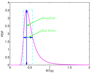
Figure 3: Depicts the relationship between a PDF’s modal value and its half width.

We use HW, instead of SD, because PDF’s fat tail heavily influences the value of the latter. Both HW and power-law exponent depend on at least one shape parameter. Unlike the simple dependence of the latter (see Eqs. (3) and (5)), the parametric dependence of HW can be quite complex. For GIGa, for instance, the expressions for HW and MPDF for $\mu=0$ are as follows:

$$\begin{array}[]{rcl}HW&=&\beta\left\{\left[-\frac{\alpha\gamma+1}{\gamma}W_{0}\left(-\frac{2^{-\frac{\gamma}{\alpha\gamma+1}}\left(\frac{\alpha\gamma+1}{e\gamma}\right)^{\left(\frac{\alpha\gamma+1}{\gamma}\right)}}{\alpha+\gamma^{-1}}\right)\right]^{-\frac{1}{\gamma}}\right.\\ &&\quad\left.-\left[-\frac{\alpha\gamma+1}{\gamma}W_{-1}\left(-\frac{2^{-\frac{\gamma}{\alpha\gamma+1}}\left(\frac{\alpha\gamma+1}{e\gamma}\right)^{\left(\frac{\alpha\gamma+1}{\gamma}\right)}}{\alpha+\gamma^{-1}}\right)\right]^{-\frac{1}{\gamma}}\right\}\end{array}$$ (10)

$$MPDF=\frac{\gamma\left(\frac{\alpha\gamma+1}{e\gamma}\right)^{\left(\frac{\alpha\gamma+1}{\gamma}\right)}}{\beta\Gamma(\alpha)}$$ (11)

where $W_{0}$ and $W_{-1}$ are the two branches of the Lambert W function and $\Gamma$ is the gamma function.

5 Application to Dyslexia

We now use GIGa and LNP distributions to decide whether the difference between the dyslexic and control groups, described in detail in (Holden et al., 2014), reduces to rescaling or implies a more significant neurophysiological difference. Holden et al. contrasted the performance of children with dyslexia and matched age-appropriate readers in four tasks with varied reading related requirements. In the above reference, each subject was fitted with an LNP and parameters thus obtained were averaged between subjects, which is a standard technique currently in use. Based on the latter, the conclusion was drawn that the difference between the control and dyslexic groups is consistent with rescaling in the reading intensive task. This method averaged parameters of individual fits, and was not sensitive enough to detect systematic between-group differences in the non-reading tasks.

Here we use a less-traditional averaging procedure, based on aggregation analysis of Sec. 3, that reveals additional information. Namely, we combine the RT of the entire control group into a single sample and do the same for the dyslexic group. We believe that such an averaging procedure may be more sensitive to subtle trends in clinical studies, as discussed in terms of random variates in Sec. 3.

In particular, we analyze the flanker and the arithmetic tasks (Holden et al., 2014). While the former is a better test of a lower-level skill, the latter emphasizes the higher-level cognitive activity. We argue that while the flanker is consistent with the rescaling, arithmetic task is not. Once we fitted the distributions with GIGa and LNP, we used a bootstrap procedure (Efron & Tibshirani, 1994) to determine the confidence intervals and distributions of the parameters.

5.1 Flanker

In Figure 4, the left column corresponds to GIGa fitting and the right column to LNP fitting. From top to bottom, we present the distribution fits of the control and dyslexic groups, followed by comparison of the two fitted distributions and then the same two now rescaled to have a unity mean. We then show the bootstrap-obtained distribution of $\alpha\gamma+1$ and $\beta$ for GIGa and of ($\alpha+1$) and $x_{P}$ for LNP. Clearly, the test is quite consistent with rescaling and similarity of underlying neurophysiology.

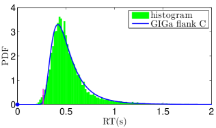
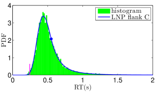
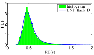
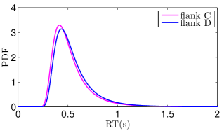
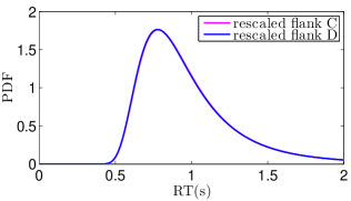
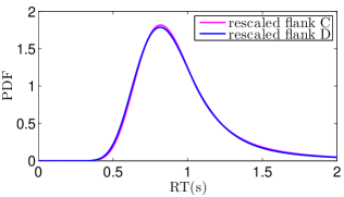
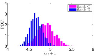
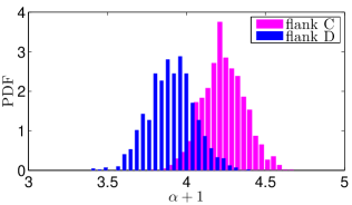
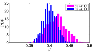
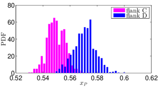
Figure 4: Flanker test. Left column: GIGa; right column: LNP. Row one: fits of control group; row two: fits of dyslexic group; row three: fits from first and second row compared; row four: same as in row three, rescaled to unity mean; row five: bootstrap-obtained distributions for power-law exponents ($\alpha\gamma+1$) and ($\alpha+1$); row six: bootstrap-obtained distributions for scale parameters $\beta$ and $x_{P}$.

5.2 Arithmetic

We now present the same figure, Figure 5, for the arithmetic test. Additionally, in Table 5, we show confidence intervals for the power-law tail exponent and the scale parameters of GIGa and LNP. For comparison purposes, we also give the confidence intervals for the flanker test in Table 6. Confidence intervals in Table 5 and 6 reflect the confidence level of $95\%$.

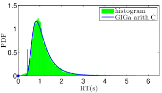
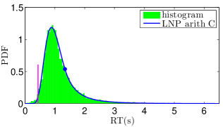
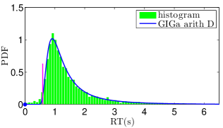
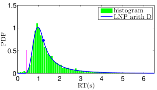
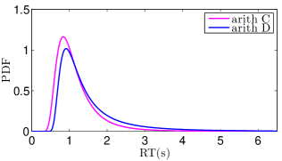
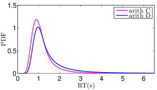
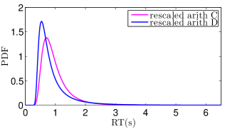
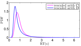
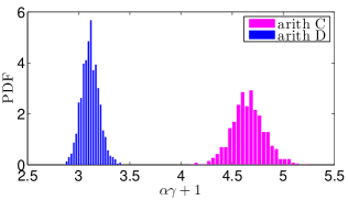
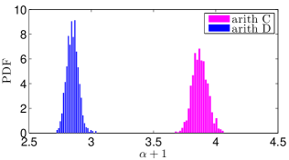
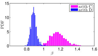
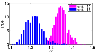
Figure 5: Arithmetic test. Left column: GIGa; right column: LNP. Row one: fits of control group; row two: fits of dyslexic group; row three: fits from first and second row compared; row four: same as in row three, rescaled to unity mean; row five: bootstrap-obtained distributions for power-law exponents ($\alpha\gamma+1$) and ($\alpha+1$); row six: bootstrap-obtained distributions for scale parameters $\beta$ and $x_{P}$.

Table 5: Confidence intervals for arithmetic Test

GIGA CI of ($\alpha\gamma+1$)
Control	(4.469,	5.114)
Dyslexia	(2.948,	3.291)

LNP CI of ($\alpha+1$)
Control	(3.741,	3.984)
Dyslexia	(2.783,	2.994)

GIGA CI of $\beta$
Control	(1.074,	1.490)
Dyslexia	(0.817,	0.949)

LNP CI of $x_{P}$
Control	(1.277,	1.391)
Dyslexia	(1.165,	1.359)

Table 6: Confidence intervals for flanker Test

GIGA CI of ($\alpha\gamma+1$)
Control	(4.530,	5.281)
Dyslexia	(4.381,	4.944)

LNP CI of ($\alpha+1$)
Control	(3.984,	4.512)
Dyslexia	(3.625,	4.200)

GIGA CI of $\beta$
Control	(0.370,	0.465)
Dyslexia	(0.369,	0.435)

LNP CI of $x_{P}$
Control	(0.537,	0.563)
Dyslexia	(0.554,	0.587)

Notice that when the scale parameters ”coincide” for two groups, the groups are still different if the shape parameters are different. For instance, while the $x_{P}$ confidence intervals overlap for the arithmetic test, those for ($\alpha+1$) do not (nor do they for HW, (Liu et al., , in preparation)).

Our analysis extends to the color and the word-naming tests, (Holden et al., 2014) with the former consistent with rescaling and the latter not (Liu et al., , in preparation). We should point out that, unlike word-naming, the arithmetic result is entirely unexpected.

6 Conclusions

We discussed properties of the candidate distributions with ”fat” power-law tails: stable, generalized inverse gamma and mixture lognormal-Pareto. We emphasized their shape and scale parameters, as those are crucial for interpreting similarities and differences in the underlying neurophysiology of cognition between a group of interest and a control group.

We hypothesized that when the response time distributions of the two groups can be rescaled to each other by the ratio of the mean responses, the supporting cognitive and neurophysiological organization should be interpreted as generally equivalent, but proportionally stretched or compressed in the temporal domain. For the candidate distributions (and other analytical distributions), such rescaling is achieved by rescaling of the scale parameter.

Conversely, absent the rescaling between the distributions, the neurophysiology should be generally interpreted as different. For the candidate distributions (and other analytical distributions), the difference is expressed via the difference of the shape, or shape-related, parameters.

In order to improve statistics for analysis of the similarity and difference between the two groups, we combined all the subjects of each group into a single set. This deviates from the common practice in which each subject is fitted separately and the parameters of the fits are subsequently averaged. We conjectured that each subject may be interpreted as a random variate of the response time distribution, the latter corresponding to a particular neurophysiological process. We conducted a numerical simulation to successfully test our conjecture.

We illustrated our approach on the response-time trials with dyslexic children and their control counterparts. We showed that, using the combined sets of each group for the analysis, the distributions of the dyslexic and control groups are consistent with rescaling for simpler cognitive tasks but not so for higher-level tasks. We used the distribution’s half-width and power-law tail exponent as shape parameters and bootstrap to obtain confidence intervals. We hope to extend our approach to clinical trials, such as studies of efficacy of ADHD medications (Epstein et al., 2011).

References

References

- Ancelin et al. (2006) Ancelin, M. L., Artero, S., Portet, F., Dupuy, A.-M., Touchon, J., Ritchie, K. et al. (2006). Non-degenerative mild cognitive impairment in elderly people and use of anticholinergic drugs: longitudinal cohort study. Bmj, 332, 455–459.
- Bouchaud & Mézard (2000) Bouchaud, J.-P., & Mézard, M. (2000). Wealth condensation in a simple model of economy. Physica A: Statistical Mechanics and its Applications, 282, 536–545.
- Efron & Tibshirani (1994) Efron, B., & Tibshirani, R. J. (1994). An introduction to the bootstrap. CRC press.
- Epstein et al. (2011) Epstein, J. N., Brinkman, W. B., Froehlich, T., Langberg, J. M., Narad, M. E., Antonini, T. N., Shiels, K., Simon, J. O., & Altaye, M. (2011). Effects of stimulant medication, incentives, and event rate on reaction time variability in children with adhd. Neuropsychopharmacology, 36, 1060–1072.
- Holden et al. (2014) Holden, J. G., Greijn, L. T., van Rooij, M. M., Wijnants, M. L., & Bosman, A. M. (2014). Dyslexic and skilled reading dynamics are self-similar. Annals of dyslexia, 64, 202–221.
- Holden et al. (2013) Holden, J. G., Ma, T., & Serota, R. (2013). Change is time: A comment on ”Physiologic time: A hypothesis”. Physics of Life Reviews, 10, 231–232. doi:10.1016/j.plrev.2013.04.003.
- Holden & Rajaraman (2012) Holden, J. G., & Rajaraman, S. (2012). The self-organization of a spoken word. Frontiers in psychology, 3.
- Holden et al. (2009) Holden, J. G., Van Orden, G. C., & Turvey, M. T. (2009). Dispersion of response times reveals cognitive dynamics. Psychological review, 116, 318.
- Ihlen (2013) Ihlen, E. A. (2013). The influence of power law distributions on long-range trial dependency of response times. Journal of Mathematical Psychology, 57, 215–224.
- Lam et al. (2011) Lam, H., Blanchet, J., Burch, D., & Bazant, M. Z. (2011). Corrections to the central limit theorem for heavy-tailed probability densities. Journal of Theoretical Probability, 24, 895–927.
- Limpert et al. (2001) Limpert, E., Stahel, W., & Abbt, M. (2001). Log-normal distributions across the sciences: Keys and clues. BioScience, 51.
- (12) Liu, Z., Pavlov-Garcia, O., Holden, J. G., & A., S. R. (). In preparation.
- Ma et al. (2013) Ma, T., Holden, J. G., & Serota, R. (2013). Distribution of wealth in a network model of the economy. Physica A: Statistical Mechanics and its Applications, 392, 2434–2441.
- Ma et al. (2015) Ma, T., Holden, J. G., & Serota, R. (2015). Distribution of human response times. Complexity, .
- Ma & Serota (2014) Ma, T., & Serota, R. (2014). A model for stock returns and volatility. Physica A: Statistical Mechanics and its Applications, 398, 89–115.
- Mandelbrot (2002) Mandelbrot, B. (2002). Gaussian self-affinity and fractals: Globality, the earth, 1/f noise, and R/S volume 8. Springer Science & Business Media.
- Moscoso Del Prado Martin (2008) Moscoso Del Prado Martin, F. (2008). A theory of reaction time distributions.
- Nolan (2015) Nolan, J. P. (2015). Stable Distributions - Models for Heavy Tailed Data. Boston: Birkhauser. In progress, Chapter 1 online at academic2.american.edu/jpnolan.
- Stone & Van Orden (1993) Stone, G. O., & Van Orden, G. C. (1993). Strategic control of processing in word recognition. Journal of Experimental Psychology: Human Perception and Performance, 19, 744.
- Tse et al. (2010) Tse, C.-S., Balota, D. A., Yap, M. J., Duchek, J. M., & McCabe, D. P. (2010). Effects of healthy aging and early stage dementia of the alzheimer’s type on components of response time distributions in three attention tasks. Neuropsychology, 24, 300.
- Van Orden et al. (2003) Van Orden, G. C., Holden, J. G., & Turvey, M. T. (2003). Self-organization of cognitive performance. Journal of Experimental Psychology: General, 132, 331.
- Van Orden et al. (2005) Van Orden, G. C., Holden, J. G., & Turvey, M. T. (2005). Human cognition and 1/f scaling. Journal of Experimental Psychology: General, 134, 117.
- Van Rooij et al. (2013) Van Rooij, M. M., Nash, B. A., Rajaraman, S., & Holden, J. G. (2013). A fractal approach to dynamic inference and distribution analysis. Frontiers in physiology, 4.