Transformations of galaxies. III. Encounter dynamics and tidal response as functions of galaxy structure

Abstract

Tidal interactions between disc galaxies depend on galaxy structure, but the details of this relationship are incompletely understood. I have constructed a three-parameter grid of bulge/disc/halo models broadly consistent with $\Lambda$CDM, and simulated an extensive series of encounters using these models. Halo mass and extent strongly influence the dynamics of orbit evolution. In close encounters, the transfer of angular momentum mediated by the dynamical response of massive, extended haloes can reverse the direction of orbital motion of the central galaxies after their first passage. Tidal response is strongly correlated with the ratio $v_{\mathrm{e}}/v_{\mathrm{c}}$ of escape to circular velocity within the participating discs. Moreover, the same ratio also correlates with the rate at which tidal tails are reaccreted by their galaxies of origin; consequently, merger remnants with ‘twin tails’, such as NGC 7252, may prove hard to reproduce unless $(v_{\mathrm{e}}/v_{\mathrm{c}})^{2}\lesssim 5.5$. The tidal morphology of an interacting system can provide useful constraints on progenitor structure. In particular, encounters in which halo dynamics reverses orbital motion exhibit a distinctive morphology which may be recognized observationally. Detailed models attempting to reproduce observations of interacting galaxies should explore the likely range of progenitor structures along with other encounter parameters.

1 INTRODUCTION

Numerical studies of interacting galaxies have come far since the first efforts, but every study to date has grappled with the huge variety of encounters which are possible. In a fundamental paper, Toomre & Toomre (1972, hereafter TT) introduced a key set of parameters and illustrated how these parameters influence the outcome of a tidal encounter. Many subsequent studies have adopted similar parameterizations and explored some subset of galactic encounters. For example, a number of authors have focused on equal-mass encounters, in which both galaxies have the same initial structure, and systematically examined the tidal response as a function of encounter parameters such as initial disc orientation.

Somewhat less attention has been given to the ways in which tidal interactions depend on the internal structures of the galaxies involved. For TT, this issue was almost moot – with all the gravitating mass concentrated in a central point, all they needed to do was to vary the outer radii of their test-particle discs. Once self-consistent simulations became possible (e.g., White, 1978; Farouki & Shapiro, 1982; Barnes, 1988), the question of internal structure, and in particular the amount of dark matter, became more interesting. Dubinski, Mihos, & Hernquist (1996) simulated encounters between galaxies with various disc/halo mass ratios, and reported that only relatively low-mass haloes permitted the formation of long tidal tails. Later studies (Mihos, Dubinski, & Hernquist, 1998; Dubinski, Mihos, & Hernquist, 1999; Barnes, 1999; Springel & White, 1999, hereafter SW) examined this claim in detail, and converged on a more precise conclusion: tail length constrains potential-well shape, not disc/halo fraction (see § 1.1). But these studies largely focused on the specific question of tail formation, and paid less attention to the broader relationship between internal structure and tidal interactions.

Hierarchical galaxy formation includes stochastic elements which inevitably produce variations in galactic properties and structure. Disc galaxies display a range of rotation curves; some have gently rising profiles, while others reach a maximum at a few disc scale lengths and remain flat or gradually decline at larger radii (e.g., Casertano & van Gorkom, 1991; de Blok et al., 2008). Even within the constraints implied by the baryonic Tully-Fischer relationship (e.g. Freeman, 1999; McGaugh et al., 2000; Verheijen, 2001) there seems to be room for interesting variety, with the luminous mass fraction (including both stars and gas) varying by a factor of a few from galaxy to galaxy (Zaritsky et al., 2014). Thus in modeling tidal encounters of disc galaxies, there are good reasons to experiment with different halo structures.

Ultimately, detailed modeling of interacting galaxies may provide a way to study the initial structure of their progenitors. This could offer a unique window on halo properties, involving the dark matter as a fully dynamical participant and probing its distribution out to relatively large radii. At present, however, it’s not clear how much information can be extracted from modeling; for example, can dynamical modeling correctly diagnose halo structure, or do the plethora of parameters available insure that the observations can be matched tolerably well even with the wrong choice of halo model? To frame this question more tightly, suppose we knew the orbital and viewing geometry of an interacting system – under this very idealized set of circumstances, can detailed modeling yield a correct picture of halo structure?

1.1 Tail formation

Distinctive tidal features form when galactic discs are subject to relatively brief but violent tides during close encounters (TT). Unlike the rather broad tidal bulges that the Moon creates on Earth, the tidal features extracted from spinning galactic discs are often quite narrow and extended. In a typical encounter, each disc produces two such features: a bridge toward the galaxy’s companion, and a tail stretching in the opposite direction. The most pronounced bridges and tails develop when a galaxy’s spin angular momentum is parallel to the orbital angular momentum of a passing companion. In this case, the angular velocities of individual stars resonate with the angular velocity of the companion, creating a strong response (TT; D’Onghia et al. 2010). An extended tail can only form if the companion’s mass is comparable to or exceeds the victim’s; otherwise, the result is a weaker ‘counter-arm’ which soon falls back into the parent galaxy. In systems like NGC 4676 where both galaxies exhibit tails, this implies that the two galaxies have comparable masses.

SW, building on earlier work by Mo, Mao, & White (1998) and Barnes (1999), showed that even under otherwise favorable circumstances, discs don’t produce long tidal tails if the quantity

$$\mathcal{E}=\frac{v_{\mathrm{e}}^{2}}{v_{\mathrm{c}}^{2}}$$ (1)

exceeds a certain value. Here $v_{\mathrm{e}}$ and $v_{\mathrm{c}}$ are the escape and circular velocity, respectively, evaluated near the disc’s half mass radius; thus $\mathcal{E}$ is the ratio of the escape energy to the kinetic energy for a circular orbit. Only discs with $\mathcal{E}\lesssim 6.5$ readily form tails in equal-mass encounters. The situation for encounters with mass ratios $\mu\neq 1$ has not yet been investigated.

Figure 1: Relationship between escape velocity $v_{\mathrm{e}}$ and circular velocity $v_{\mathrm{c}}$. The solid curve shows a $\Phi=-1/R$ potential. The dashed line, tangent to the curve $\Phi(R)$ at radius $R$, intercepts the $R=0$ axis at $\Phi=\Phi(R)-v_{\mathrm{c}}^{2}$. Dot-dash lines at $\Phi=-1$ and $-2$ help to show that $\frac{1}{2}v_{\mathrm{c}}^{2}=v_{\mathrm{e}}^{2}$ for a Keplerian potential. The dotted curve is a Hernquist (1990) potential, $\Phi=-1/(R+a)$, with scale radius $a={\color[rgb]{0,0,0}0.5}$; this is simply the $-1/R$ curve translated to the left by $a$.

This criterion can be directly visualized on a plot of gravitational potential $\Phi(R)$. Fig. 1 illustrates the relationship between $v_{\mathrm{e}}^{2}=-2\Phi(R)$ and $v_{\mathrm{c}}^{2}=R\,d\Phi/dR$. For a Keplerian potential, $v_{\mathrm{e}}^{2}=2v_{\mathrm{c}}^{2}$ everywhere, so $\mathcal{E}_{\mathrm{Kep}}=2$. This implies that test-particle discs in Keplerian potentials can easily form tidal tails, as TT originally demonstrated. For comparison, consider the Hernquist (1990) model, which has a potential of the form $\Phi(R)\propto 1/(R+a)$, where $a>0$ is the scale radius. It’s evident that $v_{\mathrm{e}}^{2}>2v_{\mathrm{c}}^{2}$ everywhere, and $\mathcal{E}{\color[rgb]{0,0,0}(R)}=2(R+a)/R$, interpreted just for this paragraph as a function of $R$, becomes arbitrarily large in the $R\ll a$ limit. The condition $\mathcal{E}\lesssim 6.5$ is satisfied at radii $R\gtrsim 0.44a$. Thus, to produce tails, a disc of test particles embedded in a Hernquist potential with scale radius $a$ must have a median radius $R_{1/2}\gtrsim 0.44a$. Similar considerations apply to other extended mass distributions, including those with discs of finite mass. In general, $\mathcal{E}(R)$ approaches the Keplerian value $\mathcal{E}_{\mathrm{Kep}}=2$ from above as $R\to\infty$. This implies that more extended discs have smaller values of $\mathcal{E}$, and therefore form tails more easily.

This simple example suggests that modeling will indeed be able to provide some information on halo structure – the very existence of long tidal tails implies, at a minimum, that some galaxies have discs with $\mathcal{E}\lesssim 6.5$. But further work is needed to find out how much more we can learn.

1.2 Outline

To determine what detailed modeling of tidal encounters might teach us, it seems reasonable to investigate encounters between a variety of galaxy models. This is not an entirely new direction; in particular, SW and Dubinski, Mihos, & Hernquist (1999) provide significant precedents. The present study expands on their work, testing a wide range of galaxy models, classifying tidal responses, and systematically comparing tidal features. Like these studies, it shares one key limitation: the two galaxies in each encounter are ‘twins’, with the same mass and the same internal structure. However, a fairly wide range of internal structures are employed, producing a variety of interaction dynamics and tidal configurations.

This paper is organized as follows. Section 2 first develops a set of galaxy models and identifies those which are stable and therefore suitable raw material for further investigations, and next describes the set of encounters simulated using these galaxies. Section 3 presents simulation results, focusing on orbital evolution, while Section 4 covers characterization of tidal features. Section 5 takes up the hypothetical modeling problem just described, and asks how well tidal response can constrain halo structure. Conclusions appear in Section 6. Technical details are described in Appendix A, while tests of isolated galaxy models appear in Appendix B.

2 INITIAL CONDITIONS

2.1 Galaxy Models

Each galaxy model contains three collisionless components, initialized with explicit density profiles; in order of decreasing mass, these are the halo, disc, and bulge. The halo is composed of dark matter, while the disc and bulge are composed of luminous material (stars), but all are assumed to obey the same $N$-body equations of motion.

1. The halo has a Navarro, Frenk, & White (1996, 1997, hereafter NFW) profile, parameterized by a total mass $M_{\mathrm{h}}$, a scale radius $a_{\mathrm{h}}$, and a taper radius $b_{\mathrm{h}}$. Within $R\leq b_{\mathrm{h}}$, the profile is

$$\rho_{\mathrm{h}}(R)=\frac{M_{\mathrm{h}}(a_{\mathrm{h}})}{4\pi(\ln(2)-\frac{1}{2})R(a_{\mathrm{h}}+R)^{2}}\,,$$ (2)

where $M_{\mathrm{h}}(a_{\mathrm{h}})$ is the mass within $a_{\mathrm{h}}$. For $R>b_{\mathrm{h}}$, the density profile tapers off exponentially, using the functional form devised by SW. The taper radius $b_{\mathrm{h}}$ is usually called the ‘virial radius’ and identified with $R_{200}$, the radius within which the average density of the halo is $200$ times the critical density of the universe (NFW). This identity constrains the scaling of numerical models to physical units, but isn’t directly relevant for the present calculations, which treat the tapered NFW profile as a convenient functional form. In addition, the NFW profile is used ‘as is’, without adiabatic compression; this is further discussed in § 2.1.1.

2. The disc has an exponential-isothermal profile, parameterized by mass $M_{\mathrm{d}}$, inverse scale length $\alpha_{\mathrm{d}}$, and scale height $z_{\mathrm{d}}$:

$$\rho_{\mathrm{d}}(R,z)=\frac{M_{\mathrm{d}}}{4\pi\alpha_{\mathrm{d}}^{2}z_{\mathrm{d}}}\,e^{-R\alpha_{\mathrm{d}}}\,\mathrm{sech}^{2}(z/z_{\mathrm{d}})\,.$$ (3)

No outer limit is imposed on the disc profile. In the present experiments, discs account for $75$ percent of the luminous material. The scale height is independent of $R$ and is fixed at $z_{\mathrm{d}}=0.125/\alpha_{\mathrm{d}}$ for all models.

3. The central bulge has a Jaffe (1983) profile, parameterized by mass $M_{\mathrm{b}}$ and scale radius $a_{\mathrm{b}}$:

$$\rho_{\mathrm{b}}(R)=\frac{M_{\mathrm{b}}a_{\mathrm{b}}}{4\pi R^{2}(a_{\mathrm{b}}+R)^{2}}\,.$$ (4)

Bulges account for the other $25$ percent by mass of the luminous material, so $M_{\mathrm{b}}=\frac{1}{3}M_{\mathrm{d}}$. The bulge scale radius is taken to be $a_{\mathrm{b}}=0.16a_{\mathrm{h}}$ in all experiments. Such a compact bulge has little direct effect on the dynamics of tidal interactions, but it helps to stabilize the disc against bar instabilities. In $N$-body simulations the $r^{-4}$ tail of the bulge profile presents some difficulties, since the outermost body has radius $\sim Na_{\mathrm{b}}$; as described in Barnes (2012), it’s convenient to smoothly taper (4) at large $R$.

The galaxy models used in this paper form a three-dimensional grid. Fig. 2 presents circular velocity profiles for the full set of $3\times 3\times 5=45$ bulge/disc/halo models considered here. In this and subsequent figures, this grid is laid out in two dimensions, with the ratio of halo mass within $a_{\mathrm{h}}$ to total luminous mass increasing from left to right, and the radial scale of the disc relative to the halo increasing from top to bottom. This grid contains a wide variety of models, including some which may fall outside the gamut of real galaxies. The rest of this section tries to place these models in the context of recent descriptions of galaxy formation in $\Lambda$CDM cosmologies.

Figure 2: Rotation curves for the B/D/H galaxy models. Each panel shows the rotation curve for a different galaxy model, with the luminous fraction $f_{\mathrm{L}}$ and halo concentration $c_{\mathrm{h}}$ specified along the top, and the disc compactness, $\alpha_{\mathrm{d}}a_{\mathrm{h}}$, specified along the right. Black curves are total circular velocities, while the green, blue, and red curves show the contributions of the bulges, discs, and haloes, respectively. Radii are normalized to $a_{\mathrm{h}}$, the halo’s scale radius, while velocities are normalized to $v_{\mathrm{h}}{\color[rgb]{0,0,0}=\sqrt{GM_{\mathrm{h}}(a_{\mathrm{h}})/a_{\mathrm{h}}}}$, the halo’s circular velocity at $R=a_{\mathrm{h}}$. Estimated values of $\lambda$ are calculated from (5). Models above the heavy blue line are generally too unstable to be used for encounter simulations.

The first and arguably the most fundamental parameter is the luminous mass fraction, $f_{\mathrm{L}}=(M_{\mathrm{b}}+M_{\mathrm{d}})/(M_{\mathrm{b}}+M_{\mathrm{d}}+M_{\mathrm{h}})$. In $\Lambda$CDM models consistent with WMAP and Planck, baryons comprise $16\pm 1$ percent of the matter (Hinshaw et al., 2013; Planck Collaboration et al., 2015). If all the baryons in a proto-galaxy were incorporated into a galactic disc and bulge then it would be appropriate to set $f_{\mathrm{L}}\simeq 0.16$. This value is almost certainly too high in view of the evident inefficiency of galaxy formation, as illustrated by observations of massive outflows from star-forming galaxies (e.g. Pettini et al., 2001; Steidel et al., 2010; Martin et al., 2012) and the large reservoirs of gas in rich galaxy clusters (e.g. Giodini et al., 2009). To explore trends with luminous fraction, experiments are run with $f_{\mathrm{L}}=0.2$, $0.1$, and $0.05$. The high end of this range, which is beyond the canonical value of $0.16$, is included to make contact with earlier experiments (e.g., Barnes, 1988, 1992). At the low end, $f_{\mathrm{L}}=0.05$ allows the luminous discs to retain some degree of self-gravity; still lower values, although astrophysically possible, effectively relegate the discs to test-particle status.

The second parameter is the halo concentration, $c_{\mathrm{h}}=b_{\mathrm{h}}/a_{\mathrm{h}}$. In $\Lambda$CDM simulations, the concentration of a halo depends on its formation history; haloes which have recently been restructured by major mergers typically have low concentrations, while those which have been quietly accreting for a long time have higher concentrations (e.g., Zhao et al., 2003; Ludlow et al., 2014). As noted above, (2) is used here as a convenient function, and the value of $b_{\mathrm{h}}$ is not tied directly to the cosmology. To sample a range of both realistic and counterfactual possibilities, values of $c_{\mathrm{h}}=4$, $8$, and $16$ are adopted; the first of these makes contact with earlier experiments which typically used rather small haloes.

The third parameter is the disc ‘compactness’, $\alpha_{\mathrm{d}}a_{\mathrm{h}}$ (the slightly nonstandard terminology is intended as a reminder that larger values of $\alpha_{\mathrm{d}}a_{\mathrm{h}}$ imply smaller discs, and vice versa). Values of $\alpha_{\mathrm{d}}a_{\mathrm{h}}=1.875$, $2.4$, $3.0$, $3.75$, and $4.8$ are used here. Note that these values are almost equally spaced logarithmically by factors very close to $\sqrt[3]{2}$. The range of $\alpha_{\mathrm{d}}a_{\mathrm{h}}$ values adopted here is dictated by two considerations.

First, not all of the models in Fig. 2 are stable. In particular, the disc-dominated models at the upper left of the grid rapidly develop strong bars. Appendix B describes stability tests for these galaxy models which set an upper limit on $\alpha_{\mathrm{d}}a_{\mathrm{h}}$ for a given choice of $f_{\mathrm{L}}$ and $c_{\mathrm{h}}$.

Second, very extended discs require large amounts of angular momentum. The angular momentum of a proto-galaxy is quantified by the dimensionless spin parameter

$$\lambda=\frac{J_{\mathrm{pg}}\sqrt{-E_{\mathrm{pg}}}}{GM_{\mathrm{pg}}^{5/2}}\,.$$ (5)

Here $M_{\mathrm{pg}}$, $J_{\mathrm{pg}}$, and $E_{\mathrm{pg}}$ are the proto-galaxy’s mass, angular momentum, and binding energy, respectively. In a simple picture of galaxy formation where discs form via gradual gas cooling within initially well-mixed and undifferentiated haloes (e.g., Fall & Efstathiou, 1980; Fall, 1983; Dalcanton, Spergel, & Summers, 1997; Mo, Mao, & White, 1998), these parameters may be estimated as follows. Neglect of accretion or outflows implies $M_{\mathrm{pg}}=M_{\mathrm{b}}+M_{\mathrm{d}}+M_{\mathrm{h}}$. Gas and dark matter are both subject to the same tidal torques (Hoyle, 1949; Peebles, 1969), and therefore should have the same specific angular momenta; assuming that the gas conserves angular momentum as it cools, $J_{\mathrm{pg}}/M_{\mathrm{pg}}=J_{\mathrm{d}}/M_{\mathrm{d}}$, where the right-hand side refers to the present disc. Finally, $E_{\mathrm{pg}}$ may be computed by assuming that the virialized proto-galaxy had the same radial distribution as the present halo.

Fig. 2 shows $\lambda$ values for each model, estimated using (5). In each column of this figure, $\lambda$ scales in rough proportion to $\alpha_{\mathrm{d}}^{-1}$; larger discs have more angular momentum. Simulations of structure formation in $\Lambda$CDM indicate that the spin parameter has a median value $\lambda_{\mathrm{med}}\simeq 0.034$, with some dependence on the algorithm used to define bound haloes (e.g., Bett et al., 2007); the distribution of $\lambda$ is rather wide, with 10th and 90th percentiles differing by a factor of $\sim 5$ (Mo, van den Bosch, & White, 2010). Most of the stable galaxy models in Fig. 2 have estimated $\lambda$ values exceeding $\lambda_{\mathrm{med}}$. However, given the width of the $\lambda$ distribution, it seems reasonable to view models with $\lambda\lesssim 0.08$ as generally consistent with simple pictures of galaxy formation in a $\Lambda$CDM universe (e.g., Mo, Mao, & White, 1998).

Nearly two-thirds of the models in the bottom two rows of Fig. 2 have estimated $\lambda$ values exceeding $0.08$. These models will be retained as a hedge against the possibility that the simple picture of galaxy formation invoked above is incomplete. For example, outflows may preferentially eject gas with low angular momentum (Brook et al., 2011; Genel et al., 2015), leaving material with high angular momentum to form discs; alternately, accretion via cold flows may introduce gas with high angular momentum (Stewart et al., 2013) which can build up larger discs. Retaining these models yields a total of $36$ stable galaxy models which will be used for encounter simulations.

2.1.1 Halo compression

Unlike earlier studies (e.g., Mo, Mao, & White 1998; SW), the NFW halo profiles in the present models were not modified to account for adiabatic compression by the gravitational field of the disc and bulge. This is partly a matter of convenience; the process of model construction and any auxiliary calculations are more straightforward if the NFW profile is used without modification. However, there are two additional considerations.

1. The standard halo compression algorithm, due to Blumenthal et al. (1986), is based on the assumption that the halo responds as if its constituent particles are on circular orbits. In practice, this may not be a good assumption; haloes formed by gravitational collapse are likely to have radially biased velocity distributions. A number of studies (Barnes, 1987; Sellwood, 1999; Wilson & Kalnajs, 2002; Gnedin et al., 2004; Sellwood & McGaugh, 2005; Tissera et al., 2010) have found that the Blumenthal et al. (1986) algorithm significantly overestimates the response of initially isotropic or radially-biased haloes. Sellwood & McGaugh (2005) describe an algorithm, based on Young (1980)’s treatment of adiabatic compression in spherical systems, which describes the compression of such haloes more accurately.

2. Observational evidence suggests that the effect of galaxy formation on halo structure is considerably more complex than models of adiabatic compression imply. Dwarf disc galaxies, in particular, appear to have haloes with constant-density cores or cusps shallower than the $r^{-1}$ NFW profile (e.g., Côté, Carignan, & Freeman, 2000; de Blok, McGaugh, & Rubin, 2001; de Blok, Bosma, & McGaugh, 2003; Swaters et al., 2003). One possible explanation invokes what might be called non-adiabatic decompression of dark haloes in response to explosive ejection of baryonic material (e.g., Governato et al., 2012, and references therein). While compressed NFW haloes fit the rotation curves of massive galaxies fairly well (e.g., Sellwood & McGaugh, 2005; Dutton et al., 2011), direct evidence for massive outflows (e.g. Pettini et al., 2001; Steidel et al., 2010; Martin et al., 2012) shows that baryons don’t always accumulate in a gradual and monotonic fashion.

In sum, the standard recipe for halo compression should probably be replaced by a more accurate treatment including both adiabatic and non-adiabatic processes. However, it’s not yet clear what effects must be included. The exploratory calculations presented here are relatively insensitive to the details of the inner halo profile; including halo compression would not alter the main results of this study.

2.1.2 Initialization

The bulge, disc, and halo components of each model are initialized in approximate dynamical equilibrium with their combined gravitational field. For the halo and bulge, a smoothing formalism (Barnes, 2012) is used to compute their contributions to the gravitational field, while the disc’s contribution is approximated by an equivalent spherical mass distribution. Isotropic distribution functions for the bulge and halo are computed using Eddington’s formula, and sampled to obtain position and velocity coordinates (e.g., Barnes, 2012). The disc is initialized using Jeans’ equations to constrain moments of the velocity distribution (e.g., Barnes & Hibbard, 2009). While this procedure is somewhat ad hoc, it’s very fast; this is an advantage when many simulations are planned. The large number of experiments dictates relatively modest particle numbers: $N_{\mathrm{b}}=16384$, $N_{\mathrm{d}}=49152$, and $N_{\mathrm{h}}=65536$ to $311296$. However, the simulations are large enough to study tidal responses. Further details of the simulations are given in Appendix A.

2.2 Encounter Survey

All of the encounters described here have the same mass ratio, $\mu=1$, initial orbital eccentricity, $e=1$, and encounter geometry. The two galaxy models in each encounter have identical parameters. One disc lies exactly in the orbital plane and rotates in the same direction that the two galaxies pass each other; this disc therefore has inclination $i_{1}=0^{\circ}$. The other disc has an inclination of $i_{2}=71^{\circ}$ and a nominal pericentric argument, relative to the idealized Keplerian orbit, of $\omega_{2}=+30^{\circ}$. Thus, while both discs have prograde ($i<90^{\circ}$) encounters, the second disc is tilted by a fairly large angle, generating rather different tidal features.

The primary encounter survey spans a grid of four parameters. Three describe the galaxy model and were introduced in § 2.1. The remaining parameter specifies the pericentric separation of the initial orbit, $r_{\mathrm{p}}/a_{\mathrm{h}}$. All four of these parameters are dimensionless quantities; to summarize, the values used are

$$\begin{array}[]{r@{\quad}c@{\quad}l@{\quad}l@{\quad}l@{\quad}l@{\quad}l@{\quad}}f_{\mathrm{L}}&=&0.2,&&0.1,&&0.05,\\ c_{\mathrm{h}}&=&16,&&8,&&4,\\ \alpha_{\mathrm{d}}a_{\mathrm{h}}&=&1.875,&2.4,&3.0,&3.75,&4.8,\\ r_{\mathrm{p}}/a_{\mathrm{h}}&=&0.5,&&1.0,&&2.0\,.\\ \end{array}$$ (6)

Since only $36$ of the $45$ galaxy models are stable, the primary sample contains a total of $108$ different encounters.

In addition to the primary sample, $24$ encounters with pericentric separations interpolating between the values in (6) were run. This secondary sample contains six galaxy models; three with luminous fraction $f_{\mathrm{L}}=0.1$, disc compactness $\alpha_{\mathrm{d}}a_{\mathrm{h}}=3.0$, and halo concentration $c_{\mathrm{h}}=16,8,4$, and three with $f_{\mathrm{L}}=0.05$, $\alpha_{\mathrm{d}}a_{\mathrm{h}}=4.8$, and $c_{\mathrm{h}}=16,8,4$. Pericentric separations of

$$r_{\mathrm{p}}/a_{\mathrm{h}}=0.625,0.8,1.25,1.6\,,$$ (7)

when combined with the primary grid, provide finer coverage in $r_{\mathrm{p}}/a_{\mathrm{h}}$. This secondary sample is useful in exploring trends with pericentric separation for the six models it includes.

An encounter’s pericentric separation $r_{\mathrm{p}}$ is related to the angular momentum $J_{\mathrm{orb}}$ of its initial parabolic orbit:

$$J_{\mathrm{orb}}=\sqrt{GM_{\mathrm{g}}^{3}r_{\mathrm{p}}}\,,$$ (8)

where $M_{\mathrm{g}}$ is the mass of a single galaxy. This angular momentum is presumably generated by tidal torques acting on the two galactic haloes as they collapse out of the Hubble flow, reach their maximum separation, and fall back towards each other; the amount of momentum torques generate implies an upper limit to $r_{\mathrm{p}}$. To estimate this limit, assume that haloes merge without significant ejection of mass, angular momentum, or binding energy; the remnant will then have spin parameter

$$\lambda_{\mathrm{orb}}=\frac{J_{\mathrm{orb}}\sqrt{-E_{\mathrm{orb}}}}{G(2M_{\mathrm{g}})^{5/2}}\,,$$ (9)

where $E_{\mathrm{orb}}$ is binding energy of the initial configuration. Since initially the orbit is parabolic and the galaxies are well-separated, $E_{\mathrm{orb}}$ is just twice the binding energy of a single galaxy, $E_{\mathrm{g}}=-KGM_{\mathrm{g}}^{2}/a_{\mathrm{h}}$, where the form factor $K$ has a weak dependence on $c_{\mathrm{h}}$, $f_{\mathrm{L}}$, and $\alpha_{\mathrm{d}}a_{\mathrm{h}}$. Evaluating this factor numerically yields

$$\lambda_{\mathrm{orb}}\simeq(0.067\pm 0.017)\sqrt{r_{\mathrm{p}}/a_{\mathrm{h}}}\,,$$ (10)

where the given uncertainty encompasses the full range of values possible for all $36$ stable galaxy models. The upshot is that encounters with $r_{\mathrm{p}}/a_{\mathrm{h}}=0.5$ to $2$ have orbital angular momenta within the range which can be produced by the tidal torque mechanism. Wider encounters are probably rare, requiring special circumstances to generate so much angular momentum. On the other hand, closer encounters can occur and are certainly worth investigating.

3 ORBITAL DYNAMICS

A tidal encounter between two extended, self-gravitating objects transfers energy and momentum from relative motion to internal degrees of freedom. As a result, the orbits of interacting galaxies evolve and eventually decay, culminating in a merger.

3.1 Encounter characterization

While Keplerian trajectories neatly parameterize the ingoing orbits of a pair of initially well-separated galaxies, they don’t describe the circumstances of deeply interpenetrating encounters very well. In such encounters, galaxies begin diverging from their initial orbits even before their first passage. Such divergence is to be expected: once they are close enough to interpenetrate, the mutual gravitational acceleration of two spatially extended structures is less than that of two equivalent point masses. With less acceleration to bend their trajectories, the galaxies undergo a first passage both wider and slower than their initial Keplerian orbit would imply.

Accurate orbital trajectories are needed to examine this effect. At every time-step, the central position $\overline{\mathbf{r}}_{j}$ and velocity $\overline{\mathbf{v}}_{j}$ of galaxy $j$ were computed by averaging over a fixed set $\mathcal{C}_{j}$ of tightly-bound bodies. These sets were constructed by initially sorting the bulge bodies of galaxy $j$ by binding energy, and using the $25$ percent most tightly bound as $\mathcal{C}_{j}$. While some diffusion in binding energy occurs due to $N$-body scattering and dynamical evolution, the most tightly-bound quartile of the bulge is stable and provides a robust determination of galaxy position, capable of tracking the motion of the dynamical centre through at least the first three pericentric passages. (Galaxy velocities are determined a bit less accurately since the bodies in $\mathcal{C}_{j}$ have a larger spread in velocity than in position, but in practice the inner quartile of each bulge averages over enough bodies to provide good results.) As these trajectories are computed, it’s straightforward to identify the instant $t_{\mathrm{p1}}$ of closest approach; a snapshot of the system at this time is saved for subsequent analysis. Let $r_{\mathrm{p1}}=|\overline{\mathbf{r}}_{2}-\overline{\mathbf{r}}_{1}|$ and $v_{\mathrm{p1}}=|\overline{\mathbf{v}}_{2}-\overline{\mathbf{v}}_{1}|$ be the separation and relative velocity at time $t_{\mathrm{p1}}$; these may be compared to the corresponding Keplerian values, $r_{\mathrm{p}}$ and $v_{\mathrm{p}}$, respectively.

Figure 3: Scatter plot showing the relationship between the normalized pericentric separation $r_{\mathrm{p1}}/r_{\mathrm{p}}$ and the interpenetration parameter $R_{x}/r_{\mathrm{p}}$. All $132$ encounters are plotted. The large symbols show results for $R_{x}=R_{1/2}$, the half-mass radius, while smaller symbols to the left and right show results for $R_{x}=R_{1/4}$ and $R_{3/4}$, respectively. Symbol type indicates halo concentration, while color indicates initial pericentric separation (see Fig. 6 for a complete key). The dashed line shows a power law fit, with a slope of $0.308$.

The ratio $R_{\mathrm{1/2}}/r_{\mathrm{p}}$, where $R_{\mathrm{1/2}}$ is the galactic half-mass radius, quantifies the degree of interpenetration which would occur if the galaxies remained on their initial trajectories. Despite its somewhat hypothetical formulation, this ratio is a good predictor of orbital behavior (e.g., Farouki & Shapiro, 1982; Barnes, 1992). For example, it predicts the actual pericentric separation $r_{\mathrm{p1}}$; as Fig. 3 shows, all $132$ simulations presented here follow a fairly tight power-law of the form $r_{\mathrm{p1}}/r_{\mathrm{p}}\simeq(R_{\mathrm{1/2}}/r_{\mathrm{p}})^{0.308}$. Similar relationships are obtained using $R_{1/4}$ and $R_{3/4}$, the radii enclosing one quarter and three quarters of the mass, respectively, although the former correlation shows more scatter. In the limit of very wide, non-interpenetrating passages, $r_{\mathrm{p1}}/r_{\mathrm{p}}$ presumably approaches $1$ from above, so these empirical power-laws can’t be universal. However, Fig. 3 nicely illustrates how initial pericentric separation and halo concentration jointly influence first passage via the degree of interpenetration. Deviations from Keplerian trajectories are largest for close encounters (red: $r_{\mathrm{p}}/a_{\mathrm{h}}=0.5$) between extended galaxies (triangles: $c_{\mathrm{h}}=16$), and smallest for wide encounters (blue: $r_{\mathrm{p}}/a_{\mathrm{h}}=2$) between compact galaxies (stars: $c_{\mathrm{h}}=4$).

Figure 4: Scatter plot showing measured pericentric separation $r_{\mathrm{p1}}$ and relative velocity $v_{\mathrm{p1}}$, normalized by the corresponding values for the initial Keplerian orbit, $r_{\mathrm{p}}$ and $v_{\mathrm{p}}$. As in Fig. 3, all $132$ encounters are plotted, symbol type indicates halo concentration, and color indicates pericentric separation. In addition, three open circles represent encounters of heavily softened ‘point’ masses. The dashed line shows the relationship $j_{\mathrm{p1}}=0.838\,j_{\mathrm{orb}}$.

Fig. 4 displays measured pericentric separations $r_{\mathrm{p1}}$ and relative velocities $v_{\mathrm{p1}}$, normalized by the corresponding values for the initial Keplerian orbits. This plot reveals a simple pattern: across the entire set of $132$ self-consistent encounters, the specific angular momentum at pericentre $j_{\mathrm{p1}}=r_{\mathrm{p1}}v_{\mathrm{p1}}\simeq(0.838\pm 0.025)\,j_{\mathrm{orb}}$, where $j_{\mathrm{orb}}=J_{\mathrm{orb}}/(2M_{\mathrm{g}})$ is the specific angular momentum of the initial orbit. This factor of $\sim 0.84$ appears because tidal interactions, operating even before first passage, have transferred about $16$ percent of the initial angular momentum from orbital motion to internal degrees of freedom within each galaxy. It seems remarkable, given the range of encounters studied here, that such a consistent fraction of orbital angular momentum is lost. For comparison, the three open symbols in this figure show experiments with very heavily softened point masses, which can be thought of as rigid mass profiles. Because they cannot deform, their orbits do not decay, and their encounters conserve orbital momentum exactly.

A final point concerns the argument of pericentre $\omega_{2}$ for the second ($i_{2}=71^{\circ}$) discs. The nominal value of $\omega_{2}=+30^{\circ}$ would imply that the first ($i_{1}=0^{\circ}$) galaxy passes through the plane of this disc some time before pericentre. However, because these self-consistent orbits deviate quite strongly from their Keplerian counterparts, the actual positions of the two galaxies at $t_{\mathrm{p1}}$ typically places the first galaxy’s centre close to the second galaxy’s spin plane. For this sample of encounters, the second disc’s effective argument of pericentre is $\omega_{2}^{\mathrm{eff}}{\color[rgb]{0,0,0}{}\simeq 0^{\circ}\pm 15^{\circ}}$, instead of $+30^{\circ}$ (see supplement Fig. 1). There’s no analogous effect for the first disc, but only because this disc lies in the orbital plane; if it had a nonzero inclination, it too would have $\omega_{1}^{\mathrm{eff}}\neq\omega_{1}$. The effective argument of pericentre may provide a better parameterization of encounter geometry when comparing tidal responses of different encounters. As TT showed, tidal responses are typically strongest for $\omega\sim 0^{\circ}$ and weakest for $\omega\sim\pm 90^{\circ}$. In the present study, since $\omega_{2}^{\mathrm{eff}}\sim 0^{\circ}$, most of these discs should respond in a fairly uniform manner, with variations in $\omega_{2}^{\mathrm{eff}}$ playing only a minor role.

3.2 Orbit evolution

All of these galaxy pairs become bound during their first passage, and subsequently fall back together. The time between the first and second passages, $\Delta t_{\mathrm{p12}}$, is comparable to the orbital period at the galactic half-mass radius, $t_{1/2}$, since $t_{1/2}$ is the time-scale for a galaxy to rearrange its mass distribution. Fig. 5 plots $\Delta t_{\mathrm{p12}}/t_{1/2}$ against the interpenetration parameter $R_{1/2}/r_{\mathrm{p}}$ (also see supplement Fig. 2). Basically, all $132$ encounters have their second passage at a time $\Delta t_{\mathrm{p12}}\simeq(0.5\mathrm{\,to\,}2)\,t_{1/2}$ after their first passage. Moreover, the variation in $\Delta t_{\mathrm{p12}}/t_{1/2}$ is strongly correlated with the degree of interpenetration, with the closest encounters resulting in the most rapid orbit decay.

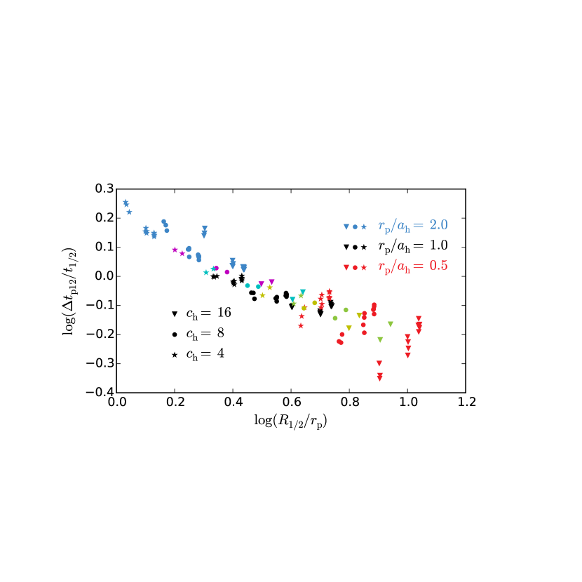
Figure 5: Scatter plot showing time between first and second passage, normalized by the orbital period at the half-mass radius, versus the interpenetration parameter. As in Fig. 3, all $132$ encounters are plotted, symbol type indicates halo concentration, and color indicates pericentric separation.

Fig. 6 presents relative orbital trajectories for the entire sample of $132$ encounters, grouped into $36$ ensembles – one ensemble for each stable galaxy model. In these plots, the position of galaxy $2$ is shown with respect to galaxy $1$. All encounters initially travel in a clockwise direction. After first passage the galaxies are trapped on bound orbits, which typically attain apocentric separations of $\sim 12a_{\mathrm{h}}$ or less for even the widest encounters (blue curves; $r_{\mathrm{p}}/a_{\mathrm{h}}=2$). Luminous fraction $f_{\mathrm{L}}$ and halo concentration $c_{\mathrm{h}}$ both systematically influence orbital trajectory. Decreasing $f_{\mathrm{L}}$ shifts the position of the apocentre counter-clockwise, while decreasing $c_{\mathrm{h}}$ reduces the apocentric distance. On the other hand, disc compactness has almost no influence on these trajectories; for the $f_{\mathrm{L}}=0.2$ encounters, apocentric separation decreases slightly as $\alpha_{\mathrm{d}}a_{\mathrm{h}}$ is reduced, but no discernible effect is seen for smaller values of $f_{\mathrm{L}}$. This is not very surprising since the disc is a small fraction of the total mass.

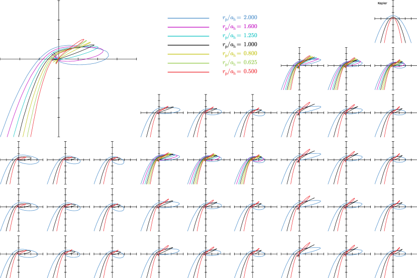
Figure 6: Relative orbital trajectories of all $132$ encounters, plotted on the orbital plane. The encounters are grouped into $36$ ensembles with identical $f_{\mathrm{L}}$, $c_{\mathrm{h}}$, and $\alpha_{\mathrm{d}}a_{\mathrm{h}}$ values; line color indicates $r_{\mathrm{p}}/a_{\mathrm{h}}$. The layout of this figure matches Fig. 2; in the region previously occupied by unstable models, the ensemble with $(f_{\mathrm{L}},c_{\mathrm{h}},\alpha_{\mathrm{d}}a_{\mathrm{h}})=(0.1,8,3.0)$ is replotted on a larger scale for better visibility; fine details in other panels may be best viewed electronically. The small plot labeled ‘Kepler’ shows representative parabolic trajectories. Tick marks are spaced $4a_{\mathrm{h}}$ apart.

Rather more surprising is the reversal of orbital angular momentum following close passages of extended, massive haloes. This can be seen, for example, in the large plot for ensemble $(f_{\mathrm{L}},c_{\mathrm{h}},\alpha_{\mathrm{d}}a_{\mathrm{h}})=(0.1,8,3.0)$, where the oval curves traced by the wider encounters give way to increasingly hairpin turns at apocentre as $r_{\mathrm{p}}/a_{\mathrm{h}}$ is reduced. For the two closest members of the ensemble (green and red curves, for $r_{\mathrm{p}}/a_{\mathrm{h}}=0.625$ and $0.5$, respectively), the hairpin becomes a self-crossing loop, and galaxy $2$ falls back toward galaxy $1$ on a slightly counter-clockwise path. This curious behavior is not limited to members of this ensemble; it appears uniformly in every encounter with $f_{\mathrm{L}}\leq 0.1$ and $r_{\mathrm{p}}/a_{\mathrm{h}}=0.5$.

Another view of this effect is provided by Fig. 7, where the top and bottom panels show the separation between the galaxy centres $r$ and their specific orbital angular momentum $j$, respectively. Prior to first passage, $j$ merely fluctuates about the specific orbital angular momentum $j_{\mathrm{orb}}$; these fluctuations are due to ongoing exchanges of linear momentum between each centre and its own surrounding halo, magnified by the long lever arm afforded by large values of $r$. At first pericentre, $j$ has declined by only $\sim 18$ percent, consistent with Fig. 4, but shortly thereafter it drops dramatically as the tidally distorted haloes rapidly absorb angular momentum. This process continues well past first pericentre, with $j$ finally changing sign when the galaxy centres are $\sim 6a_{\mathrm{h}}$ apart and continuing to decrease until somewhat after first apocentre. At second pericentre the whole process appears to repeat in a roughly self-similar pattern, with $j$ changing sign yet again shortly after $t_{\mathrm{p2}}$.

Figure 7: Evolution of an encounter, with parameters $(f_{\mathrm{L}},c_{\mathrm{h}},\alpha_{\mathrm{d}}a_{\mathrm{h}},r_{\mathrm{p}}/a_{\mathrm{h}})=(0.05,16,4.8,0.5)$, which exhibits reversal of orbital angular momentum. Top panel shows separation as a function of time $t$, normalized by $t_{1/2}$, the orbital period at the galactic half-mass radius. The dotted curve is an equaivalent Keplerian orbit. Bottom panel shows the specific orbital angular momentum normalized to its initial value; note that $j$ changes sign after both the first and second passages.

What accounts for this ‘extinction beyond the zero’ of angular momentum? Any explanation invoking dynamical friction will fail; friction can reduce angular momentum asymptotically to zero, but not beyond. Instead, consider a parabolic ($e=1$), nearly head-on encounter of two extended, massive haloes; after deeply interpenetrating, they will evolve toward a prolate structure tumbling very slowly in the plane of their initial orbits. Now suppose these haloes each contain a self-gravitating component (traced, for example, by a bulge) which, being much smaller in radius, experiences the same encounter as hyperbolic and grazing. These bulges will be strongly deflected and will, for a time, separate in a direction making a significant angle to the major axis of the prolate structure formed by the two haloes. As they do so, they encounter a steep gravitational gradient which pushes them back toward the major axis even before it halts their outward motion; as a result, their orbital angular momenta reverse. Fig. 8 shows the mass distribution of the encounter in Fig. 7 just before first apocentre, at a time when the specific angular momenta of the galaxies is rapidly decreasing; the misalignment of the outer, roughly prolate bar and the inner dumbbell will clearly torque the latter in a counter-clockwise direction.

Fig. 9 shows the relationship between orbital angular momentum at second pericentre, $j_{\mathrm{p2}}/j_{\mathrm{orb}}$, and the degree of interpenetration at first passage, $R_{1/2}/r_{\mathrm{p}}$. All encounters with $j_{\mathrm{p2}}/j_{\mathrm{orb}}<0$ have undergone extinction beyond zero. The most striking examples involve deeply interpenetrating encounters between extended ($c_{\mathrm{h}}=16$) and massive ($f_{\mathrm{L}}=0.05$) haloes; this is entirely consistent with the scenario outlined above. In contrast, this form of orbit decay is almost never observed for encounters with $f_{\mathrm{L}}=0.2$ (open symbols in Fig. 9); typically, low-mass halos can’t exert enough gravitational torque to drive $j$ beyond the zero.

Figure 8: Mass distribution of encounter in Fig. 7 shortly before first apocenter, projected onto the orbital plane. Contours enclose $25$, $50$, and $75$ precent of the mass in projection. Red and blue curves are galaxy trajectories.

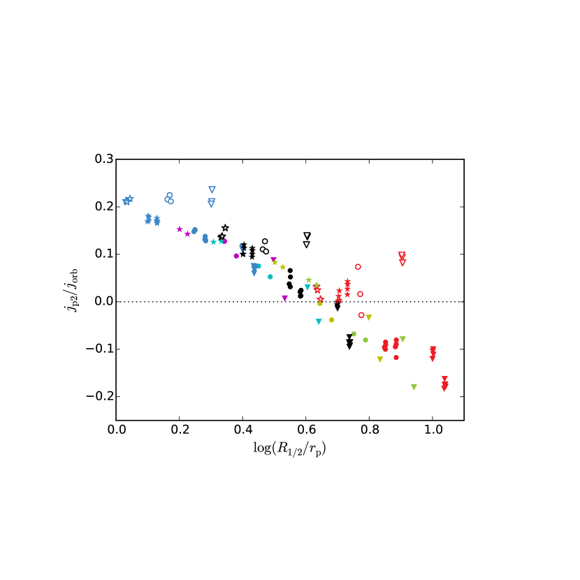
Figure 9: Relationship between interpenetration factor and orbital angular momentum at second pericentre. Symbol types and colors follow Fig. 3; in addition, encounters with $f_{\mathrm{L}}=0.2$ are plotted as open symbols, while those with $f_{\mathrm{L}}\leq 0.1$ are plotted as solid symbols. Note that the $f_{\mathrm{L}}=0.2$ encounters are often outliers in what is otherwise a fairly tight relationship; and do not, for any combination of parameters used here, exhibit significant ‘extinction beyond the zero’.

Such violent orbit decay contradicts the assumption that the ‘final encounters’ of merging systems involve roughly circular orbits (e.g. Tecza et al., 2000; Romanowsky & Fall, 2012). For a wide range of initial conditions, the second passages of these equal–mass pairs are nearly head-on and intensely disruptive, and a third passage and merger follow very shortly thereafter. This point has not been widely recognized. Tsatsi et al. (2015) find a similar effect in a simulated major merger, although in the case they present the orbital angular momentum did not reverse until after the second passage. It’s unclear if encounters of unequal–mass pairs can also evolve in this fashion.

4 DISC RESPONSE

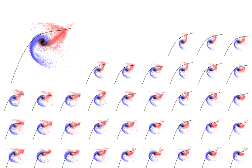
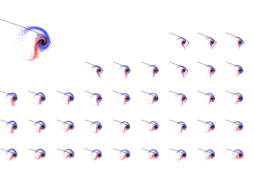
Figure 10: Disc response one rotation period after pericentre for $r_{\mathrm{p}}/a_{\mathrm{h}}=1$ encounters. Top and bottom grids show $i=0^{\circ}$ and $i=71^{\circ}$ discs, respectively, viewed face-on and scaled to keep $\alpha_{\mathrm{d}}^{-1}$ constant. The layout of each grid mirrors Fig. 6, with the $(f_{\mathrm{L}},c_{\mathrm{h}},\alpha_{\mathrm{d}}a_{\mathrm{h}},r_{\mathrm{p}}/a_{\mathrm{h}})=(0.1,8,3.0,1)$ discs replotted on a larger scale. Black curves show companion trajectores; a filled dot marks actual pericentre. Grey circles show the radius $5\alpha_{\mathrm{d}}^{-1}$. Colors indicate tidal classification; tails and bridges bodies are shown in blue and red, respectively, while regions containing both are rendered black. Note that colors are assigned to all bodies, but only those beyond $5\alpha_{\mathrm{d}}^{-1}$ are counted as tidal features. See supplement Figs. 3 and 4 for other $r_{\mathrm{p}}/a_{\mathrm{h}}$ values.

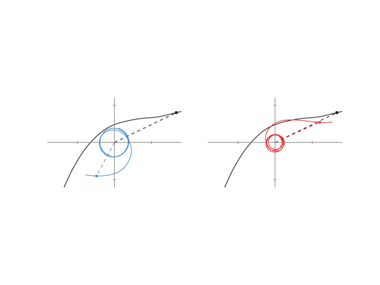
Figure 11: Classification of bodies in tidal features. Each panel is plotted with respect to the centre of the parent galaxy; tick marks are $10\alpha_{\mathrm{d}}^{-1}$ apart. The black curve shows the trajectory of the companion galaxy, while the colored curve shows the trajectory of the body being classified. In each panel, filled squares show positions when the body reaches its maximum radius for the time interval $t_{\mathrm{p1}}<t<t_{\mathrm{tid}}$, and the angle between the dashed lines is $\psi_{\mathrm{a}}$. Left: tail trajectory ($\cos\psi_{\mathrm{a}}<0$). Right: bridge trajectory ($\cos\psi_{\mathrm{a}}>0$).

Fig. 10 illustrates the relationship between galaxy structure and tidal response. At top right in the upper grid are very compact discs situated deep within massive halos. These discs have been subject to in-plane yet fast and relatively distant encounters and develop fairly symmetrical tidal features. Moving down these columns, disc size increases and the tidal response, while stronger, becomes less symmetric, with bridges becoming noticeably less coherent. Moving to the left reduces the potential well depth and encounter speed, both factors contributing to increased tidal response. In many of these slower cases, the bridge actually catches up with and even ‘wraps around’ the companion.

Inclined passages are presented in the bottom grid of Fig. 10. The discs in the upper right of this grid again develop moderately symmetric tidal features. Moving across this grid a different morphology emerges, with the largest discs exhibiting off-center ring-like features. These rings result from roughly perpendicular and deeply interpenetrating passages (Lynds & Toomre, 1976; Theys & Spiegel, 1977); see Fig. 3 of Barnes (1992) for an illustration of this sort of ring-making.

4.1 Identification of tidal features

SW measured the strength of tidal features by counting all bodies at distances $R>10\alpha_{\mathrm{d}}^{-1}$ from their parent galaxy’s centre of mass. They defined $T(t)$ to be the fraction of disc bodies satisfying this criterion at time $t$, and took the maximum value, $T_{\mathrm{eff}}$, as an effective measure of tidal response. However, this strategy has some limitations which became apparent in analyzing the wide range of tidal encounters studied here. First, while SW’s criterion is appropriate when focusing on long tidal tails, some discs exhibit definite tidal features which fit almost entirely within a radius $R<10\alpha_{\mathrm{d}}^{-1}$. Second, the peak value, while useful to show that elongated tidal features occur, does not address the duration of their visibility. Third, SW’s criterion counts tail and bridge bodies indiscriminately. In order to make accurate statements about, e.g., the production of tidal tails in different encounters, some method of sorting bodies into tidal features is necessary.

On a dynamical basis, tidal features should develop roughly one rotation period after pericentric passage. Thus, rather than seeking the instant when such features are maximized, each system is analyzed at time $t_{\mathrm{tid}}=t_{\mathrm{p1}}+t_{\mathrm{rot}}$, where $t_{\mathrm{p1}}$ is the actual time of first pericentre, and $t_{\mathrm{rot}}$ is the rotation period at radius $R=2\,\alpha_{\mathrm{d}}^{-1}$. This radius encloses $\sim 59$ percent of the disc mass, so $t_{\mathrm{rot}}$ is close to the median rotation period and provides a good overall measure. Direct inspection of individual discs at this time confirms that $R>10\alpha_{\mathrm{d}}^{-1}$ is too strict. A variety of criteria based on some combination of each body’s initial radius, current radius, and maximum radius were tested, but in the end it proved most straightforward to count body $i$ as part of a tidal feature if

$$R_{i}{\color[rgb]{0,0,0}(t_{\mathrm{tid}})}>5\alpha_{\mathrm{d}}^{-1}\,,$$ (11)

where $R_{i}(t)=|\mathbf{r}_{i}(t)-\overline{\mathbf{r}}_{j}(t)|$ is the distance between body $i$ and the centre of its parent galaxy $j$. The ‘optical radii’ of disc galaxies typically extend to $\sim 5\alpha_{\mathrm{d}}^{-1}$, so (11) basically identifies tidal features as material beyond the optical radius. A light grey circle superimposed on each image in Fig. 10 shows the radius $R=5\alpha_{\mathrm{d}}^{-1}$. In some cases, bridges and tails continue inward to smaller radii, while in others the discs themselves appear to extend slightly beyond, but on the whole this seems to be a reasonable working definition of tidal material.

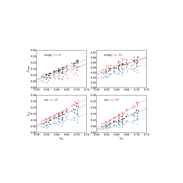
Figure 12: Scatter plots showing amount of tidal material versus ${\color[rgb]{0,0,0}\eta_{\mathrm{esc}}=}\sqrt{{\color[rgb]{0,0,0}2}/\mathcal{E}}$ for the primary sample of $108$ encounters, broken down by feature classification and disc inclination. Here, $f_{\mathrm{bridge}}$ and $f_{\mathrm{tail}}$ are the fractions of disc bodies classified as bridges and tails, measured one rotation period after first pericentre. As in Fig. 3, color indicates $r_{\mathrm{p}}/a_{\mathrm{h}}$, while symbol type indicates $c_{\mathrm{h}}$. Solid lines are linear fits for different $r_{\mathrm{p}}/a_{\mathrm{h}}$ values. Note that the panel for the $i=71^{\circ}$ bridge (top right) has a $y$-axis range one-quarter the range of the other three panels.

Having identified the bodies belonging to tidal features, the next step is to classify them as members of bridges or tails. Fig. 11 illustrates the classification algorithm, which works by analyzing individual trajectories. Follow each body from time $t_{\mathrm{p1}}$ until time $t_{\mathrm{tid}}$, and let $t_{\mathrm{a}}$ be the instant when the body’s distance from its parent is greatest (in many but not all cases, $t_{\mathrm{a}}=t_{\mathrm{tid}}$). At time $t_{\mathrm{a}}$, construct unit vectors $\widehat{\mathbf{n}}_{\mathrm{a}}$ and $\widehat{\mathbf{q}}_{\mathrm{a}}$ from the parent to the companion and the body, respectively, and let $\cos\psi_{\mathrm{a}}=\widehat{\mathbf{n}}_{\mathrm{a}}\cdot\widehat{\mathbf{q}}_{\mathrm{a}}$. Bodies which are on the side opposite the companion at $t_{\mathrm{a}}$ have $\cos\psi_{\mathrm{a}}<0$ and are classified as tail particles, while those on the same side have $\cos\psi_{\mathrm{a}}>0$ and are classified as bridge particles. Fig. 10 uses colors to indicate tidal classifications, with tails in blue and bridges in red.

Fig. 12 plots fractions of disc bodies in tidal features, organized by disc inclination and feature classification. Instead of using $\mathcal{E}$ as defined by (1), the horizontal axis is ${\color[rgb]{0,0,0}\eta_{\mathrm{esc}}=}\sqrt{{\color[rgb]{0,0,0}2}/\mathcal{E}}=\sqrt{2}\,v_{\mathrm{c}}/v_{\mathrm{e}}$. Up to a constant factor, $\eta_{\mathrm{esc}}$ is just the ratio of circular to escape velocity; following SW, this ratio is evaluated at radius $R=2\,\alpha_{\mathrm{d}}^{-1}$. This parameterization is useful because it produces roughly linear trends with $f_{\mathrm{tail}}$; moreover, the normalization insures that a Keplerian potential yields $\eta_{\mathrm{esc}}=1$, which serves as a convenient reference. Note that SW’s criterion $\mathcal{E}\lesssim 6.5$ is equivalent to $\eta_{\mathrm{esc}}\gtrsim 0.55$.

In Fig. 12, symbol color indicates pericentric separation $r_{\mathrm{p}}/a_{\mathrm{h}}$, and the solid lines are linear fits for $r_{\mathrm{p}}/a_{\mathrm{h}}={\color[rgb]{0,0,0}0.5}$ (red), ${\color[rgb]{0,0,0}1.0}$ (black), and ${\color[rgb]{0,0,0}2.0}$ (blue). These plots reveal some interesting relationships. As SW found, the parameter $\mathcal{E}$ (or equivalently, ${\color[rgb]{0,0,0}\eta_{\mathrm{esc}}}$) is strongly correlated with tidal fraction (see also supplement Fig. 5). This correlation is particularly striking for tidal tails, while for bridges the scatter is considerably larger. For tails, the second parameter which determines tidal fraction is pericentric separation; $f_{\mathrm{tail}}$ increases monotonically as $r_{\mathrm{p}}/a_{\mathrm{h}}$ decreases. This makes sense, since closer encounters produce stronger tides; indeed, this plot suggests that still closer encounters may yield even larger tail fractions. Inclination $i$ enters as a third parameter, influencing the slope of the relationship between ${\color[rgb]{0,0,0}\eta_{\mathrm{esc}}}$ and $f_{\mathrm{tail}}$.

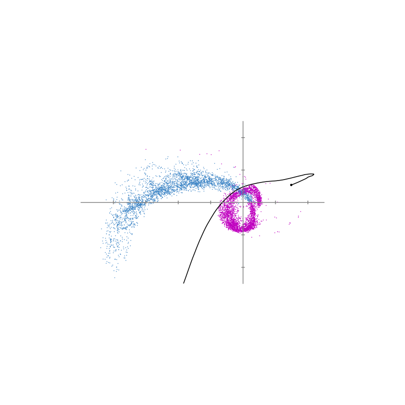
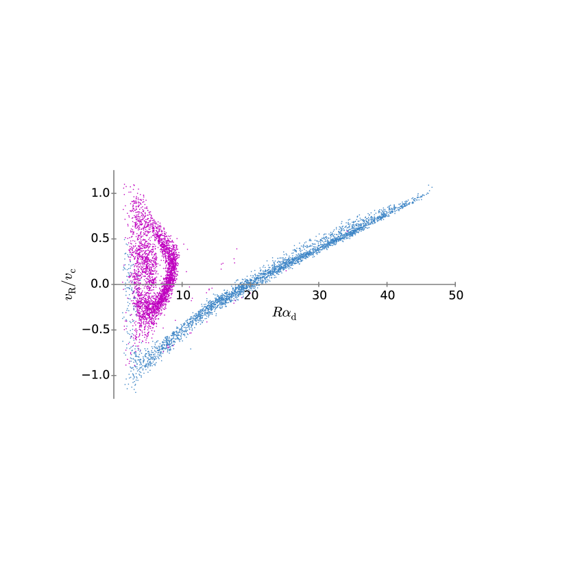
Figure 13: Reaccretion of the tidal tail from an $i=0$ disc. All the bodies plotted were classified as tail material (blue) at time $t_{\mathrm{tid}}$, but by the time shown, between first apocentre and second pericentre, roughly half have been reclassified as loop material (magenta). Left: projection onto the disc plane, with the parent galaxy at the origin; tick marks are $10\alpha_{\mathrm{d}}^{-1}$ apart. The black curve shows the companion’s relative trajectory. Right: radius $R$ versus radial velocity $v_{\mathrm{R}}$, scaled by disc scale length $\alpha_{\mathrm{d}}^{-1}$ and circular velocity $v_{\mathrm{c}}$ at $2\alpha_{\mathrm{d}}^{-1}$, respectively. All of these tail bodies remain bound to the merger remnant.

For bridges, the situation is more complex. The tidal fraction increases as $r_{\mathrm{p}}/a_{\mathrm{h}}$ is reduced from $2.0$ to $1.0$, but further reduction has the opposite effect, and the scatter about the linear fits becomes larger, especially for the $i=0$ disc. It appears that these closer passages are so deeply interpenetrating that bridge formation is suppressed, and this suppression is especially effective for in-plane encounters.

The $i=0^{\circ}$ discs typically develop comparable bridge and tail fractions, although tails are somewhat favored as $r_{\mathrm{p}}/a_{\mathrm{h}}$ decreases. On the other hand, virtually all of the tidal features from the $i=71^{\circ}$ discs are tail-dominated, often by factors of $\sim 3$ or more. This result harks back to TT’s fig. 15, which shows the bridge bodies dwindling relative to tails as inclination increases. It’s not clear why bridges are more sensitive to inclination than tails; the quasi-resonant formalism of D’Onghia et al. (2010) may be applicable to this question, but perturbation expansions to a fairly high order appear needed to address it.

4.2 Lifetimes of tidal tails

All of the galaxy models examined in this paper can produce fairly substantial bridges and tails, especially when involved in close encounters. However, these features don’t always persist. In equal-mass encounters, little or no tidal material reaches escape velocity, so tails and bridges are destined to fall back into their parent galaxies, creating complex systems of reaccreted tidal loops as shown in Fig. 13.

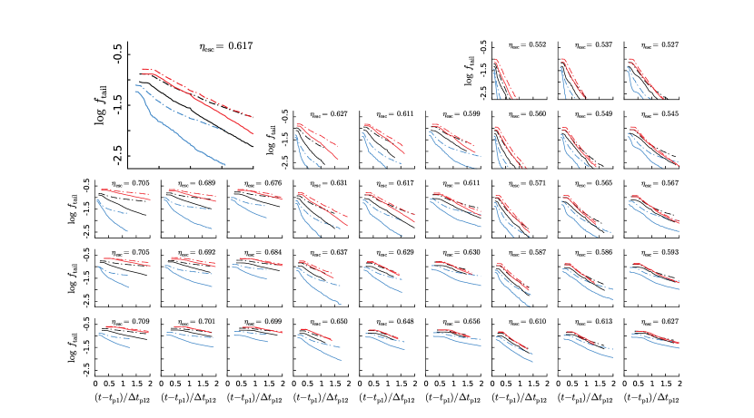
Figure 14: Evolution of tail fractions for the primary encounter sample. The layout follows Fig. 6; each panel represents an ensemble of encounters with different $r_{\mathrm{p}}/a_{\mathrm{h}}$ values, indicated by line color, and the $(f_{\mathrm{L}},c_{\mathrm{h}},\alpha_{\mathrm{d}}a_{\mathrm{h}})=(0.1,8,3.0)$ ensemble is replotted on a larger scale. Each panel plots log tail fraction against time since first pericentre, measured in units of the time between first and second passages, and the value of $\eta_{\mathrm{esc}}$ for the galaxy model used in each panel appears at the top. Dot-dashed and solid lines show tail fractions for $i=0^{\circ}$ and $i=71^{\circ}$ discs, respectively. See supplement Figs. 6 and 7 for further details on tail evolution.

This process is easier to analyze for tidal tails, which, once they are launched, evolve mostly under the influence of their parent galaxy, with relatively little ongoing interference from the companion. The basic technique is to track each tail body until its next encounter with its parent, and at that time reclassify it as belonging to a tidal loop instead of a tail. Naively, this can be done by finding the next local minimum of $R_{i}(t)$, the distance between tail body $i$ and the centre of its parent galaxy $j$. Numerical noise in $\overline{\mathbf{r}}_{j}$ may trigger reclassification prematurely when body $i$ is near apocentre; to avoid this difficulty, the minimum is required to satisfy $R_{i}(t)\leq{\color[rgb]{0,0,0}P}R_{i}^{\mathrm{max}}$, where ${\color[rgb]{0,0,0}P}=0.95$ and $R_{i}^{\mathrm{max}}=\max(R_{i}(t))$ is the tail body’s maximum distance from its parent. This simple method works well until shortly before the system’s second pericentre, but fails when the acceleration of the parent galaxy causes rapid changes in $R_{i}(t)$. A better-behaved function $R^{\prime}_{i}(t)$ can be defined by smoothly interpolating between $\overline{\mathbf{r}}_{j}$ and the system centre-of-mass position $\overline{\mathbf{r}}_{\mathrm{cm}}=(\overline{\mathbf{r}}_{1}+\overline{\mathbf{r}}_{2})/2$ as second pericentre approaches:

$$R^{\prime}_{i}(t)=|\mathbf{r}_{i}-({\color[rgb]{0,0,0}Q}\overline{\mathbf{r}}_{j}+(1-{\color[rgb]{0,0,0}Q})\overline{\mathbf{r}}_{\mathrm{cm}})|\,,$$ (12)

where ${\color[rgb]{0,0,0}Q=\min(1,d_{\mathrm{min}}\alpha_{\mathrm{d}}/5)}$ depends on the minimum distance $d_{\mathrm{min}}$ between the two galaxy centres up to time $t$. In addition, the criterion $R^{\prime}_{i}(t)\leq{\color[rgb]{0,0,0}P}R_{i}^{\mathrm{max}}$ can be tightened as the galaxies approach each other by setting ${\color[rgb]{0,0,0}P=0.6+0.35\,\exp(-(d_{\mathrm{min}}\alpha_{\mathrm{d}}/5)^{-4})}$. With these adjustments, tail reaccretion can be followed through multiple pericentric passages and ultimately merger.

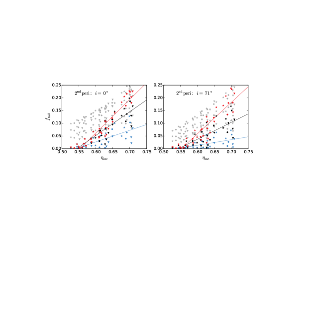
Figure 15: Scatter plots of tail fraction at second pericentre, $t=t_{\mathrm{p2}}$. As in Fig. 12, color and symbol type indicate $r_{\mathrm{p}}/a_{\mathrm{h}}$ and $c_{\mathrm{h}}$, and the solid lines are linear fits for each $r_{\mathrm{p}}/a_{\mathrm{h}}$. The light grey symbols show tail fractions at time $t=t_{\mathrm{tid}}$, one rotation period after first pericentre.

Fig. 14 shows how tail fractions $f_{\mathrm{tail}}$ evolve with time. At time $t_{\mathrm{tid}}$, when tidal features are first identified, bodies at the bases of the tails are typically near apocentre; consequently, tail fractions are initially almost constant. However, reaccretion commences as these bodies fall back toward their parents, and the tail fraction decreases monotonically thereafter. Meanwhile, the galaxies themselves, after loitering near first apocentre, fall back toward each other. By second pericentre, tail fractions have often decreased quite dramatically.

One might expect that closer encounters, which yield more tidal material and decay faster, would maximize tail fractions at later times. This is confirmed by Fig. 14; in each panel, the $r_{\mathrm{p}}/a_{\mathrm{h}}=0.5$ curves (red) start higher and usually decline more gradually than their $1.0$ (black) and $2.0$ (blue) counterparts. Another trend evident within individual panels involves disc inclination; the $i=71^{\circ}$ (solid) tails often decline more steeply than the corresponding $i=0^{\circ}$ (dot-dashed) tails.

Comparison between panels in Fig. 14 shows that reaccretion rates, indicated by the slopes of the various curves, are generally anticorrelated with $\eta_{\mathrm{esc}}$. Galaxies with $\eta_{\mathrm{esc}}\lesssim 0.55$, plotted at top of the right-hand three columns of this figure, reaccrete so rapidly that they arrive at second passage with no visible tails to speak of. Further down these columns, $\eta_{\mathrm{esc}}$ increases and the reaccretion rate diminishes. This general trend continues across the rest of the figure, and galaxies with $\eta_{\mathrm{esc}}\gtrsim 0.70$, found in the left-hand columns, typically reaccrete their tails very slowly, and often reach second passage still festooned with massive tidal tails. Note, however, that the relationship between reaccretion rate and $\eta_{\mathrm{esc}}$ has some scatter; within each group of three columns, representing different halo concentrations for a given luminous fraction, the rate of reaccretion decreases as $c_{\mathrm{h}}$ is reduced. These trends are corroborated by supplement Fig. 8, which shows the effects of $\eta_{\mathrm{esc}}$ and $c_{\mathrm{h}}$ explicitly.

The amount of tail material visible at second pericentre is further examined in Fig. 15, which reproduces the layout of the lower panels in Fig. 12. Since these encounters merge shortly after second passage (e.g., by $(t-t_{\mathrm{p1}})/\Delta t_{\mathrm{p12}}=1.25$), this plot provides an upper limit to the amount of tail material merger remnants are likely to display. The roughly linear relationships between $f_{\mathrm{tail}}$ and ${\color[rgb]{0,0,0}\eta_{\mathrm{esc}}}$ noted in Fig. 12 become steeper as a result of tail reaccretion, and halo concentration emerges as an additional parameter; both of these effects follow naturally from the trends seen in Fig. 14 and supplement Fig. 8. Merger remnants with conspicuous tails (e.g., $f_{\mathrm{tail}}\gtrsim 0.05$) appear to require $\eta_{\mathrm{esc}}\gtrsim 0.60$ (i.e., $\mathcal{E}\lesssim 5.5$); while many of the models with lower-mass haloes satisfy this condition, only those $f_{\mathrm{L}}=0.05$ models which have relatively extended discs can do so. Moreover, distant encounters frequently fail to produce remnants with $f_{\mathrm{tail}}\gtrsim 0.05$ even when $\eta_{\mathrm{esc}}\gtrsim 0.60$.

5 TIDAL CONFIGURATIONS

As shown in the previous section, the strength of the tidal response provides information about progenitor structure, but the the overall configuration of the tidal response – in other words, the strength and the morphology, taken together – may yield further constraints. SW note that such ‘constraints are potentially very powerful if dynamical modeling is combined with detailed observation’, but this idea has not yet been tested. As a first step toward this goal, we can ask if the relationship between progenitor structure and tidal configuration exhibits simple patterns which might be used to deduce halo properties?

One approach to this question is to systematically compare tidal configurations produced in encounters with different progenitor structures. A pair of encounters which consistently mimic each other’s tidal configurations will be impossible to distinguish observationally; such pairs are ‘degenerate’. In the present tests, the viewing direction and encounter geometry will be fixed a priori. This is a fairly drastic simplification; in practice, detailed modeling of interacting systems attempts to infer these geometric parameters from the observed morphology and kinematics (e.g., Barnes & Hibbard, 2009). However, in some rather limited circumstances the encounter and viewing geometry can be determined independently of other parameters (for example, an encounter between two discs with inclinations $i_{1}=i_{2}=0$, viewed face-on to the orbital plane, can be recognized as such from line-of-sight velocity data). The time since first passage, on the other hand, must be taken as an unknown.

5.1 Comparison procedure

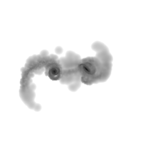
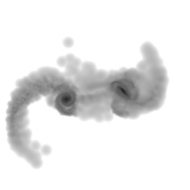
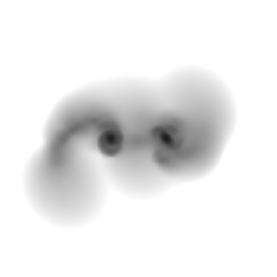
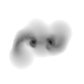
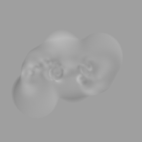
Figure 16: Two different encounters which produce similar configurations. Left: reference encounter with parameters $(f_{\mathrm{L}},c_{\mathrm{h}},\alpha_{\mathrm{d}}a_{\mathrm{h}},r_{\mathrm{p}}/a_{\mathrm{h}})=(0.1,8,3,2)$, shown at time $t_{\mathrm{ref}}=t_{\mathrm{a1}}$. Middle: comparison encounter with parameters $(0.1,16,2.4,2)$, shown at the time yielding the best match to the reference encounter. Right: difference between reference and comparison images. Top: original simulation data, yielding ${D}=0.395$. Bottom: data transformed to place galaxy centres at $(\pm 1,0,0)$ and further smoothed, yielding ${D}=0.049$.

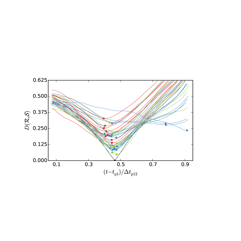
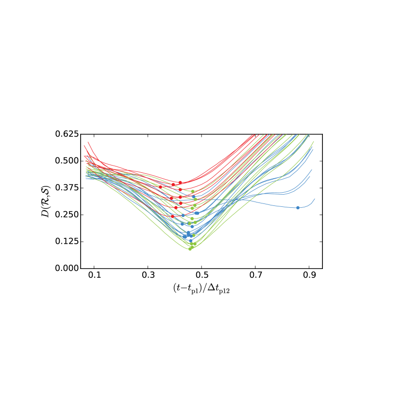
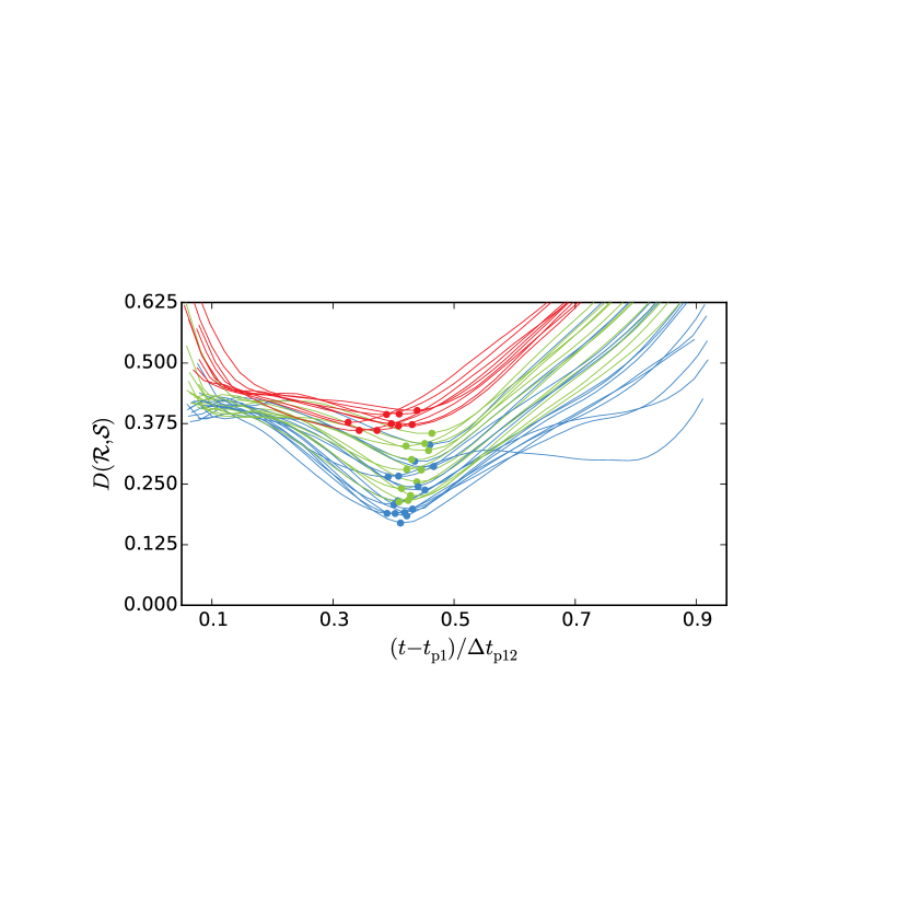
Figure 17: Time evolution of ${D}$ values computed with respect to the reference image $\mathcal{R}$ shown in the lower left of Fig. 16. The three panels show results for comparison images $\mathcal{S}$ with $r_{\mathrm{p}}/a_{\mathrm{h}}=2.0$ (top), $1.0$ (middle), and $0.5$ (bottom). Black curve: comparisons with reference encounter at other times; an exact match, ${D}=0$, occurs at $t=t_{\mathrm{a1}}$. Red, green, blue curves show matches to other encounters with $f_{\mathrm{L}}=0.2$, $0.1$, $0.05$, respectively. Minima on these curves, corresponding to best matches with the reference image, are marked.

To compare tidal configurations, simulations are turned into images, and differences are evaluated pixel by pixel. Before this can be done, some nuisance parameters must be dealt with. Pixel comparison will fail to recognize two geometrically similar shapes which don’t have the same scale, orientation, and position in the image plane (Fig. 16, top). Rather than blindly search for a transformation which minimizes pixel differences, these parameters can be eliminated by transforming the simulation data to register the centres of the two galaxies at $\overline{\mathbf{r}}_{1}=(1,0,0)$ and $\overline{\mathbf{r}}_{2}=(-1,0,0)$. (Obviously, this is only possible if the centres are well-separated; a different method is needed to compare images of merger remnants.) Next, the disc particles are projected onto the image plane and adaptively smoothed to produce a continuous grey-scale image which suppresses small-scale details but captures the overall tidal structure. To bring out tidal features, which typically have low surface density, pixel values are logarithmically transformed. Finally, two such images, with pixel values $\mathcal{A}_{k,l}$ and $\mathcal{B}_{k,l}$ where $k$ and $l$ are pixel indices, are compared by evaluating the normalized absolute difference,

$${D}(\mathcal{A},\mathcal{B})=\frac{\sum_{k,l}|\mathcal{A}_{k,l}-\mathcal{B}_{k,l}|}{\sum_{k,l}\mathcal{A}_{k,l}+\mathcal{B}_{k,l}}\,.$$ (13)

Fig. 16 presents two encounters which yield very similar tidal configurations. Here, the encounter on the left, which has parameters $(f_{\mathrm{L}},c_{\mathrm{h}},\alpha_{\mathrm{d}}a_{\mathrm{h}},r_{\mathrm{p}}/a_{\mathrm{h}})=(0.1,8,3,2)$, was chosen as the reference; it’s shown at first apocentre ($t_{\mathrm{{\color[rgb]{0,0,0}ref}}}=t_{\mathrm{a1}}$). The comparison encounter, in the middle, has parameters $(0.1,16,2.4,2)$ and is shown just slightly later; the procedure used to select the encounter and time will be described shortly. Both encounters are viewed perpendicular to the orbital plane. At the chosen times, the two galaxy pairs have slightly different position angles and distinctly different separations, and subtracting one image from another yields large residuals (top right). But these residuals are mostly due to differences in orientation and scale; once the two galaxies have been registered, the images are almost identical (bottom right). Hence, these two encounters are highly degenerate.

The match in Fig. 16 was found by a simple linear search. First, for every encounter $\mathcal{I}$, a sequence of registered images $\mathcal{S}_{{\color[rgb]{0,0,0}\mathcal{I}}}(t)$ spanning times $t$ between $t_{\mathrm{p1}}$ and $t_{\mathrm{p2}}$ was generated and stored; on average there are $\sim 70$ images per sequence. Let $\mathcal{R}(t)$ be the sequence of images generated from the reference encounter; the reference image, shown on the lower left in Fig. 16, is $\mathcal{R}(t_{\mathrm{a1}})$. Next, $\mathcal{R}(t_{\mathrm{a1}})$ was compared to every other image, yielding $D(\mathcal{R}(t_{\mathrm{a1}}),\mathcal{S}_{\mathcal{I}}(t))$ values for every encounter $\mathcal{I}$ and time $t$. Finally, these values were used to determine the time $t_{\mathcal{I}}$ when each $\mathcal{S}_{\mathcal{I}}(t)$ best matches $\mathcal{R}(t_{\mathrm{a1}})$, and the corresponding $D(\mathcal{R}(t_{\mathrm{a1}}),\mathcal{S}_{\mathcal{I}}(t_{\mathcal{I}}))$ values were sorted to identify the encounters most nearly degenerate with the reference encounter. The ${D}(\mathcal{R}(t_{\mathrm{a1}}),\mathcal{S}_{{\color[rgb]{0,0,0}\mathcal{I}}}(t))$ values are plotted as functions of $t$ in Fig. 17. The black curve was obtained by comparing $\mathcal{R}(t_{\mathrm{a1}})$ with other images from the same sequence, $\mathcal{R}(t)$; ${D}$ drops monotonically to zero when the reference image is compared to itself, and subsequently increases. Curves in other colors show the results of comparing with other encounters.

While no other encounter prefectly matches the reference image, in most cases ${D}$ reaches a definite minimum ${D}_{\mathrm{min}}$ at nearly the same stage between $t_{\mathrm{p1}}$ and $t_{\mathrm{p2}}$. The timing of these minima is determined by the time selected for the reference image. The depth of each minimum shows how closely the corresponding encounter matches $\mathcal{R}(t_{\mathrm{a1}})$. The deepest minima are found in the top panel, which compares the reference image to images of other encounters with the same pericentric separation, $r_{\mathrm{p}}/a_{\mathrm{h}}=2$. Within the top panel, most of the curves with deep minima are produced by encounters with $f_{\mathrm{L}}=0.1$ (green) or $f_{\mathrm{L}}=0.05$ (blue), while those with $f_{\mathrm{L}}=0.2$ (red) yield shallower minima. This indicates that image matching can discriminate between encounters with different luminous fractions or pericentric separations. In the top panel, two curves have minima significantly below the rest; the deeper one was used in Fig. 16. The reference encounter and its two closest matches all have $f_{\mathrm{L}}=0.1$ and $r_{\mathrm{p}}/a_{\mathrm{h}}=2$. Moreover, they have $(c_{\mathrm{h}},\alpha_{\mathrm{d}}a_{\mathrm{h}})$ values of $(16,2.4)$, $(8,3.0)$, and $(4,3.75)$; suggesting that halo concentration and disc scale can ‘trade off’ against each other to produce degenerate encounters.

Encounters which appear similar from one viewing direction don’t automatically look alike from another. To investigate this effect, registered images were constructed using four different viewing directions $(\mathbf{u}_{0},\mathbf{u}_{1},\mathbf{u}_{2},\mathbf{u}_{3})$ derived from the symmetry axes of a tetrahedron, with $\mathbf{u}_{0}$ perpendicular to the orbital plane. The upshot, at least for these encounters, is that ${D}_{\mathrm{min}}$ is fairly independent of viewing direction, although $\mathbf{u}_{0}$ is typically the most sensitive to differences in tidal configuration. This is not unexpected, since the same geometry is used for all the encounters. It’s convenient to use the average over all four directions, $\overline{D}_{\mathrm{min}}$, as an overall measure of configuration difference. For example, the encounters in Fig. 16 match well along all four directions, with $(\mathbf{u}_{0},\mathbf{u}_{1},\mathbf{u}_{2},\mathbf{u}_{3})$ yielding ${D}_{\mathrm{min}}=(0.049,0.043,0.046,0.036)$, respectively; the average is $\overline{D}_{\mathrm{min}}\simeq 0.044$.

5.2 Patterns of degeneracy

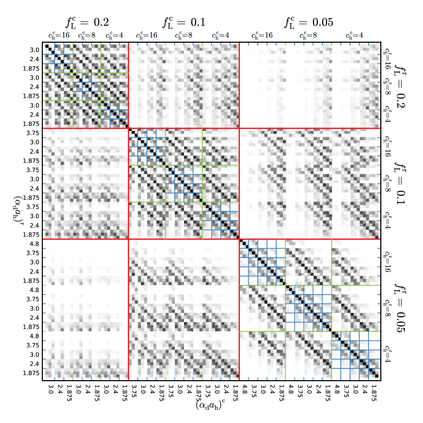
Figure 18: $108\times 108$ grid comparing tidal configurations. Each row of this grid shows the result of matching all $108$ comparison encounters to a given reference encounter. Encounters are arranged in the same order along both axes. The red, green, and blue lines separate encounters with different $f_{\mathrm{L}}$, $c_{\mathrm{h}}$, and $\alpha_{\mathrm{d}}a_{\mathrm{h}}$ values, respectively. Values of $f_{\mathrm{L}}$ and $c_{\mathrm{h}}$ are given along the top and right, while $\alpha_{\mathrm{d}}a_{\mathrm{h}}$ is given on the bottom and left; the ‘$\mathrm{r}$’ and ‘$\mathrm{c}$’ superscripts indicate reference and comparison simulations, respectively. In each $3\times 3$ group of cells, $(r_{\mathrm{p}}/a_{\mathrm{h}})^{\mathrm{c}}$ increases rightward, and $(r_{\mathrm{p}}/a_{\mathrm{h}})^{\mathrm{r}}$ increases downward. The grey value for each cell is $1-\exp(-\overline{D}_{\mathrm{min}}^{2}/0.01)$; this stretch emphasizes pairs which have similar configurations.

The same procedure has been applied to all $108$ encounters in the standard ensemble. In each case, a reference image generated at apocentre, time $t_{\mathrm{ref}}=t_{\mathrm{a1}}$, is compared to images from all other simulations, and the minimum value $\overline{D}_{\mathrm{min}}$ from each is used as a measure of degeneracy. Fig. 18, presents the results, which summarize over three million image comparisons. Here encounters are arranged in the same order along both axes; along each axis, $r_{\mathrm{p}}/a_{\mathrm{h}}$ varies fastest, $\alpha_{\mathrm{d}}a_{\mathrm{h}}$ next, $c_{\mathrm{h}}$ next, and $f_{\mathrm{L}}$ slowest. The grey value of each cell indicates the degree of degeneracy, ranging from black (identical) to white (different). The diagonal line running from upper left to lower right shows that each simulation perfectly matches itself, while dark off-diagonal cells indicate encounters which are degenerate despite having different parameters. Note that because a search over time is done to match each comparison encounter to a given reference encounter, this grid is not perfectly symmetric about the diagonal, although the asymmetry is rather subtle.

The first point Fig. 18 illustrates is that only a few pairs of encounters are as degenerate as the two in Fig. 16. This implies that it may indeed be possible to learn something about progenitor structure by analyzing tidal configurations. For example, most of the close matches are found in the three large squares recording comparisons between encounters which have identical $f_{\mathrm{L}}$ values (labeled A, B, and C in Fig. 19). Indeed, as Fig. 20 shows, pairs of encounters with identical values of $f_{\mathrm{L}}$ and $r_{\mathrm{p}}/a_{\mathrm{h}}$ account for most of the smaller $D_{\mathrm{min}}$ values in Fig. 18. In contrast, the almost complete absence of dark cells within the rectangles labeled E and E’ in Fig. 19 shows that encounters with $f_{\mathrm{L}}=0.2$ and $0.05$ produce distinctly different configurations, and thus are unlikely to be confused with each other.

A second point is that degenerate pairs don’t occur at random. Fig. 18 exhibits a good deal of structure, with most of the degenerate pairs of encounters in regions A, B, and C (Fig. 19) arranged in sequences paralleling the main diagonal. The contrast between these sequences and their surroundings is inversely correlated with luminous fraction, being strongest when the encounters are halo-dominated, as in region C, where $f_{\mathrm{L}}=0.05$.

Perhaps the most obvious of these patterns are the diagonal sequences associated with the trade off between halo concentration and disc scale noted in § 5.1. These degenerate pairs of encounters always have the same $f_{\mathrm{L}}$ and $r_{\mathrm{p}}/a_{\mathrm{h}}$, but differ in $c_{\mathrm{h}}$ and $\alpha_{\mathrm{d}}a_{\mathrm{h}}$. In Fig. 19, they form the diagonal sequences outlined in red. The origin of these patterns lies in the relationship between halo concentration and apocentric distance (see § 3.2): in effect, doubling $c_{\mathrm{h}}$ increases $r_{\mathrm{a1}}$ by an average factor of $\sim 1.26\pm 0.05$. If the disc scale is increased by the same factor, the resulting configuration will closely match the original. Fig. 20, which plots distributions of ${D}_{\mathrm{min}}$ for various sets of pairs, tests this explanation. Here the red histogram, which corresponds to the cells outlined in red in Fig. 19, derives from pairs of encounters in which $c_{\mathrm{h}}$ is doubled and $\alpha_{\mathrm{d}}a_{\mathrm{h}}$ is scaled by a factor of $\sim 0.794\simeq 1.26^{-1}$, while $f_{\mathrm{L}}$ and $r_{\mathrm{p}}/a_{\mathrm{h}}$ are held fixed. This picks out a large fraction of the most degenerate encounter pairs. In comparison, the blue histogram shows the ${D}_{\mathrm{min}}$ distribution for pairs of encounters which have similar $r_{\mathrm{a1}}\alpha_{\mathrm{d}}$ values, with $f_{\mathrm{L}}$ and $r_{\mathrm{p}}/a_{\mathrm{h}}$ again fixed. This includes most of the pairs in the red histogram, as well as a few additional pairs which are slightly less degenerate.

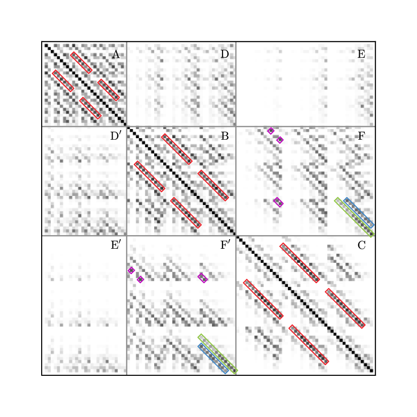
Figure 19: Key to Fig. 18, identifying regions and encounter sequences described in the text.

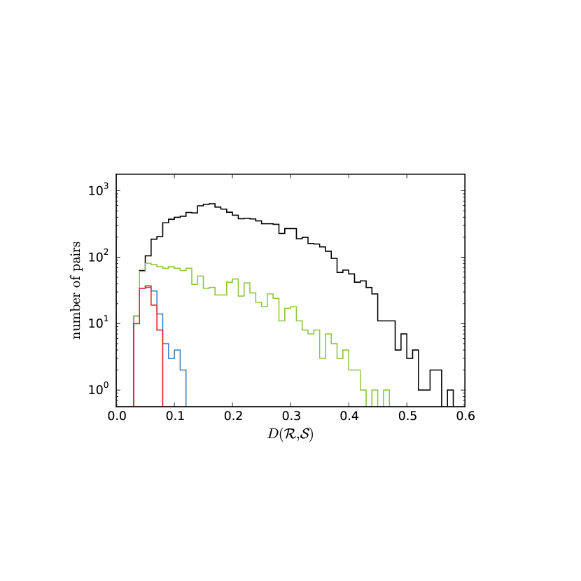
Figure 20: Distributions of $D$ values for subsets of the grid in Fig. 18. Cells on the main diagonal, which have $D=0$, are excluded from these subsets. The black histogram shows values for all off-diagonal cells, while the green one shows cells which have the same $f_{\mathrm{L}}$ and $r_{\mathrm{p}}/a_{\mathrm{h}}$. The red and blue histograms are described in the text. Note the vertical axis is logarithmic.

Turning to encounters with different values of $f_{\mathrm{L}}$, the strongest degeneracies arise when one encounter has $f_{\mathrm{L}}=0.1$ and the other has $f_{\mathrm{L}}=0.05$ (rectangles F and F’ in Fig. 19). Distinguishing between these cases is observationally interesting, since many disc galaxies appear to have $f_{\mathrm{L}}$ values in this range (Zaritsky et al., 2014). Some of the diagonal sequences in rectangles F and F’ involve pairs with relatively extended discs (ie, small $\alpha_{\mathrm{d}}a_{\mathrm{h}}$) and compact haloes (small $c_{\mathrm{h}}$). As Fig. 2 shows, the discs in these models contribute relatively little to the total circular velocity; in effect, these models are so halo-dominated that the discs could almost be massless. It’s scarcely surprising that two such encounters which have the same $c_{\mathrm{h}}$, $\alpha_{\mathrm{d}}a_{\mathrm{h}}$, and $r_{\mathrm{p}}/a_{\mathrm{h}}$ would yield similar configurations. For example, the diagonal sequence outlined in green in Fig. 19 links encounters with identical $c_{\mathrm{h}}$, $\alpha_{\mathrm{d}}a_{\mathrm{h}}$, and $r_{\mathrm{p}}a_{\mathrm{h}}$ values. Notice that the lower right end of this sequence, which represents the encounters with the most extended discs, shows the highest level of degeneracy, while encounters at the other end of the sequence are much more distinct.

Other sequences and individual matches in rectangles F and F’ are not so easily explained. Some, including the sequence outlined in blue in Fig. 19, involve pairs of encounters with similar values of $r_{\mathrm{a1}}\alpha_{\mathrm{d}}$, but this condition is neither sufficient nor necessary. A few moderately degenerate pairs of encounters, like the ones outlined in magenta, have different values of $r_{\mathrm{p}}/a_{\mathrm{h}}$. Such pairings are not seen in other regions of Fig. 19; their presence here indicates that it may not always be possible to constrain both $f_{\mathrm{L}}$ and $r_{\mathrm{p}}/a_{\mathrm{h}}$ using tidal configuration.

The patterns seen in Fig. 18 are also found when reference images are generated at other times (see supplement Fig. 9). In general, tidal configurations diverge with time, so encounters are harder to distinguish before $t_{\mathrm{a1}}$, and easier to tell apart between $t_{\mathrm{a1}}$ and $t_{\mathrm{p2}}$. Similar results are also obtained when only one of the two discs is imaged (supplement Fig. 10); in other words, the $i=0^{\circ}$ and $i=71^{\circ}$ discs independently reproduce the patterns seen here.

5.3 Morphological differences

Figure 21: Relationship between differences in tail fraction and configuration. The latter is symmetrized so that each pair of encounters is represented by a single point. Top left: result for all pairs of encounters. Top right: pairs which undergo violent orbit decay. Bottom left: pairs which undergo gentle orbit decay. Bottom right: mixed pairs. The pair marked with cross-hairs is presented in Fig. 22.

Having some idea of the factors which make a pair of encounters similar, it’s logical to ask what makes them different. One factor which obviously plays a role is the amount of tidal material; other things being equal, a larger fraction of tidal material increases the surface brightness of extended features. But does the tidal morphology also matter, or are the differences in configuration measured by (13) basically driven by differences in tidal fraction? If morphology matters, then it should be possible to find pairs of encounters, with similar tidal fractions, which nonetheless have visibly different configurations.

Comparison of configurations is more effective after tidal features have had time to develop, so this section will use a reference time half-way between first apocentre and second pericentre: $t_{\mathrm{ref}}=(t_{\mathrm{a1}}+t_{\mathrm{p2}})/2$. At such late times, tidal fractions have been substantially affected by reaccretion (§ 4.2). Since a good measure of bridge reaccretion is not yet available, tail fraction (Fig. 14) will be used as a proxy for overall tidal fraction. To further improve the discrimination of different configurations, only $\mathbf{u}_{0}$ images, face-on to the orbital plane, will be used to compute ${D}_{\mathrm{min}}$.

Let $f_{\mathrm{tail1}}^{\mathcal{I}}$ and $f_{\mathrm{tail2}}^{\mathcal{I}}$ be tail fractions for the two discs in encounter $\mathcal{I}$ at time $t_{\mathrm{ref}}$. A relative measure of the difference in tail fractions for encounters $\mathcal{I}$ and $\mathcal{J}$ is

$$\delta f_{\mathrm{tail}}^{\mathcal{IJ}}=1-\min\!\!\left[\frac{\min(f_{\mathrm{tail1}}^{\mathcal{I}},f_{\mathrm{tail1}}^{\mathcal{J}})}{\max(f_{\mathrm{tail1}}^{\mathcal{I}},f_{\mathrm{tail1}}^{\mathcal{J}})}\,,\frac{\min(f_{\mathrm{tail2}}^{\mathcal{I}},f_{\mathrm{tail2}}^{\mathcal{J}})}{\max(f_{\mathrm{tail2}}^{\mathcal{I}},f_{\mathrm{tail2}}^{\mathcal{J}})}\right]\!.$$ (14)

This quantity vanishes if both tails in $\mathcal{I}$ are as massive as their counterparts in $\mathcal{J}$, and increases if either of the corresponding tail fractions are different. Likewise, let ${D}_{\mathrm{min}}^{\mathcal{IJ}}$ be the minimum value of ${D}$ obtained when matching the reference image of $\mathcal{I}$ against the sequence of images of $\mathcal{J}$. The upper left panel in Fig. 21 plots difference in configuration against difference in tail fraction for all pairs of encounters in the standard ensemble. If configuration differences were largely driven by tail fraction, then these parameters should be highly correlated, and all pairs with $\delta f_{\mathrm{tail}}\simeq 0$ should have ${D}_{\mathrm{min}}\simeq 0$. That’s not what Fig. 21 shows; while ${D}_{\mathrm{min}}$ is correlated with $\delta f_{\mathrm{tail}}$, it still spans a considerable range even for small $\delta f_{\mathrm{tail}}$. Assuming tail fraction is a good proxy for overall response, it appears that morphology does matter.

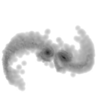
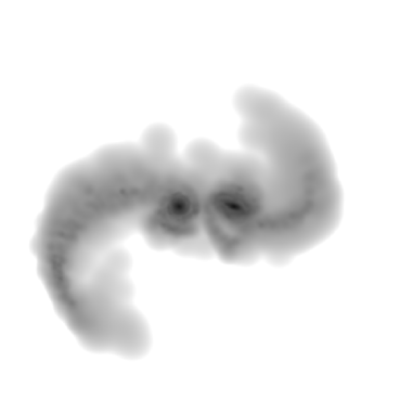
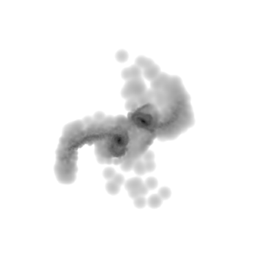
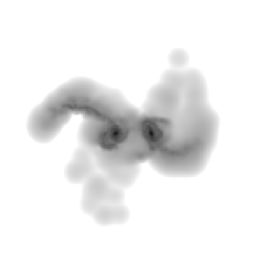
Figure 22: Two encounters with similar amounts of tail material at $t=t_{\mathrm{ref}}$ but different morphologies. Both are viewed face-on to the orbit plane. Top: encounter parameters $(f_{\mathrm{L}},c_{\mathrm{h}},\alpha_{\mathrm{d}}a_{\mathrm{h}},r_{\mathrm{p}}/a_{\mathrm{h}})=(0.2,8,2.4,2)$. Bottom: parameters $(0.1,16,3.75,0.5)$. Left: plotted to the same scale. Right: registered to $(\pm 1,0,0)$.

However, it is possible to identify subsets of the standard ensemble where differences in tail fraction are more strongly correlated with differences in configuration. The upper right panel of Fig. 21 restricts the sample to pairs where both encounters have orbits decaying ‘beyond the zero’ (§ 3.2). Specifically, the $23$ encounters in this subset have orbital angular momenta at second pericentre $j_{\mathrm{p2}}<-0.05\,j_{\mathrm{orb}}$. In this case, a definite relationship between $\delta f_{\mathrm{tail}}$ and ${D}_{\mathrm{min}}$ is evident, and ${D}_{\mathrm{min}}$ becomes fairly small as $\delta f_{\mathrm{tail}}\to 0$. For this subset, it’s plausible that differences in tail fraction account for most of the measured differences in tidal configuration; spot checks along the sequence reveal many pairs with similar shapes (see supplement Fig. 11). In other words, encounters which undergo violent orbit decay appear to have relatively homogeneous tidal morphologies over a wide range of tail fractions.

A similar result holds for encounters whose orbits decay gently. The lower left panel of Fig. 21 shows pairs with orbital angular momenta at second pericentre $j_{\mathrm{p2}}>0.15\,j_{\mathrm{orb}}$; this subset contains $22$ encounters. Again, a fairly well-defined relationship between $\delta f_{\mathrm{tail}}$ and ${D}_{\mathrm{min}}$ emerges, although in this case the relationship becomes steeper as $\delta f_{\mathrm{tail}}\to 1$. This may indicate that these gentle orbit decays, as a group, are not quite so homogeneous, but once again, spot checks show that many pairs have similar shapes even though their tail fractions may differ (supplement Fig. 12).

Finally, the lower right panel of Fig. 21 pairs violent and gentle orbit decays; that is, one member of each pair has $j_{\mathrm{p2}}<-0.05\,j_{\mathrm{orb}}$, while the other has $j_{\mathrm{p2}}>0.15\,j_{\mathrm{orb}}$. Even when both members have comparable amounts of tidal material, their morphologies are quite different, yielding ${D}_{\mathrm{min}}\gtrsim 0.2$ for almost every pair. Moreover, unlike the two previous cases, there’s only a weak correlation between $\delta f_{\mathrm{tail}}$ and ${D}_{\mathrm{min}}$; for this pair sample, differences in tail fraction don’t have that much to do with differences in configuration.

As an example, Fig. 22 contrasts the effects of gentle (top) and violent (bottom) orbit decay on tidal morphology. These two encounters, represented by the marked point in the lower right panel of Fig. 21, have very different configurations even though their tail fractions are quite similar at time $t_{\mathrm{ref}}$ ($f_{\mathrm{tail1}}=0.0691\pm 0.0017$ and $f_{\mathrm{tail2}}=0.0366\pm 0.0008$). The morphological differences seen here arise in various ways. For example, in the bottom images the discs display well-developed loops of reaccreted tail material, while such features are much less evident in the top images. This follows from the details of these two encounters. On the bottom, a close ($r_{\mathrm{p}}/a_{\mathrm{h}}=0.5$) encounter between galaxies with relatively deep potential wells ($\eta_{\mathrm{esc}}\simeq 0.627$, or $\mathcal{E}\simeq 5.08$) launched substantial tails which fell back quickly to create the loops seen here. On the top, a wider ($r_{\mathrm{p}}/a_{\mathrm{h}}=2$) encounter between galaxies with shallower wells ($\eta_{\mathrm{esc}}\simeq 0.692$, or $\mathcal{E}\simeq 4.18$) generated somewhat less massive but longer-lived tails which don’t form extensive loops of tidal material.

However, the most obvious difference in Fig. 22 is the shapes of the tails themselves. The two galaxies on the top, which barely grazed each other ($R_{1/2}/r_{\mathrm{p}}\simeq 1.47$), continue to orbit in a clockwise direction, while those on the bottom interpenetrated deeply ($R_{1/2}/r_{\mathrm{p}}\simeq 10.0$), reversed direction, and are now approaching on a counter-clockwise trajectory. These different orbital paths markedly influence the shapes of the tidal tails, which distort so as to maintain continuity with the discs which spawned them. The tails in the top encounter describe great sweeping arcs moving in the same clockwise direction as the galaxies they came from. In contrast, the the tails in the bottom encounter, especially the one from $i=0$ disc at left, have lost much of their angular momentum to the same gravitational field which reversed the orbital motions of their parent galaxies. While their tips continue to travel in a clockwise direction, these tails are predominantly falling almost radially toward the centre of the system, and the material nearest the galaxies is backtracking on plunging, counter-clockwise orbits.

The connection between tail morphology and halo mass was noted by Mihos, Dubinski, & Hernquist (1998), who report ‘[a]s we consider encounters involving galaxies with increasing halo mass, the tails become straighter and more anemic’. Earlier, Dubinski, Mihos, & Hernquist (1996) observed that tail morphology is connected to orbital angular momentum, and the bottom rows of their figs. 3 and 4 nicely illustrate the relationship between luminous fraction and tail shape. But these studies did not explicitly examine the evolution of orbital trajectories, instead linking tail shape to initial orbital shape. As the above quote indicates, they also linked tail shape and tail mass; this was probably inevitable, since the limited computing power at their disposal precluded the extensive grid of models presented in this study. Similar limitations led Dubinski, Mihos, & Hernquist (1999) to rely on test-particle simulations for the bulk of their experiments; they used dynamical friction to implement orbit decay, so their models could not reproduce the violent reversals of orbital angular momentum described here.

6 CONCLUSIONS

This study examines the relationship between the internal structure of interacting disc galaxies on the one hand and the their orbital dynamics and tidal morphology on the other. This has been accomplished by constructing a grid of bulge/disc/halo galaxy models; these models include a subset broadly consistent with $\Lambda$CDM predictions for bright disc galaxies (Mo, Mao, & White, 1998), as well as others with higher luminous fractions and proto-galactic spin parameters. Simulated encounters between identical models display a range of outcomes, which are analyzed to investigate orbital evolution, level of tidal response, and comparative tidal morphology.

Orbit decay, which is largely mediated by dynamical interactions between massive dark haloes, follows a consistent pattern for all of these equal-mass encounters. The ratio $R_{1/2}/r_{\mathrm{p}}$, which compares the galactic half-mass radius to the pericentric distance of the initial orbit, predicts many aspects of orbital evolution. These include the time-scale for orbit decay (Fig. 5) and the actual pericentric separation (Fig. 3). This ratio also correlates with the shape of the post-encounter orbits; deeply interpenetrating encounters ($R_{1/2}/r_{\mathrm{p}}\gtrsim 5$) of galaxies with dominant haloes ($f_{\mathrm{L}}\leq 0.1$) reverse direction after first passage and follow self-crossing trajectories due to violent transfer of orbital angular momentum to dark haloes.

Strength of tidal response is measured by a simple, consistent method, and a straightforward algorithm is defined to distinguish bridges and tails (Fig. 11). This method works well for the two disc orientations ($i_{1}=0^{\circ}$ and $i_{2}=71^{\circ}$, $\omega_{2}^{\mathrm{eff}}\simeq 0^{\circ}$) featured in this study, and may be useful in other cases as well. SW’s result that tidal response correlates with the escape parameter $\mathcal{E}$, defined in (1), is strongly confirmed. In particular, once tail and bridge responses can be separately measured, $f_{\mathrm{tail}}$ displays an remarkably linear relationship with $\eta_{\mathrm{esc}}$ (equivalently, with $\mathcal{E}^{-1/2}$); pericentric separation $r_{\mathrm{p}}/a_{\mathrm{h}}$ and inclination $i$ control the slope and intercept (Fig. 12). Tidal features have finite lifetimes before they’re reaccreted by their parent galaxies, and galaxies with larger $\mathcal{E}$ values reabsorb their tails faster (Figs. 14 and 15).

Overall distribution of tidal material depends on many factors, including orbit decay, tidal response, and rate of reaccretion. A systematic comparison of tidal configurations shows that some encounters have very similar morphologies and would be difficult to distinguish observationally (Fig. 16). For example, halo concentration and disc compactness are partly degenerate; a small change in the latter can mask a large change in the former. On the other hand, variations in total luminous fraction $f_{\mathrm{L}}$ have definite effects on tidal configuration which aren’t easily masked by changes in other parameters. In particular, the violent orbit decays characteristic of close encounters between massive, extended haloes yield distinctive tidal morphologies quite different from those produced in encounters between low-mass haloes (Fig. 22).

This result may seem at odds with Mihos, Dubinski, & Hernquist (1998), who found that ‘it may be difficult to distinguish between close collisions of low-mass models and wider collisions involving more massive galaxies’. However, they focused on models of the merger remnant NGC 7252, whereas the emphasis here is on tidal morphology between first and second passage. It’s likely that the earlier dynamical stage considered here provides more leverage on encounter parameters, including pericentric separation; in reconstructing tidal encounters from morphological and kinematic data, the separation and orientation of still-distinct galaxies provides useful constraints (Barnes & Hibbard, 2009).

In examining morphological indicators which yield information on halo structure, this study does not explicitly include kinematic data. Of course, line-of-sight velocities are necessary to fix an overall mass scale, and they play a key role in accurately constraining the encounter and viewing geometry of tidally interacting galaxies. However, it’s by no means clear that kinematic data would break the degeneracies noted above; the configurations and velocity fields of tidal features are intimately related, so the latter may not provide much additional information about halo properties.

The results presented here don’t necessarily create tension between observations of long-tailed interacting galaxies or twin-tailed merger remnants on the one hand, and the predictions of $\Lambda$CDM on the other. As long as a good-sized subset of the models in Fig. 2 have analogs among real galaxies, some fraction of encounters will inevitably produce objects with ‘classic’ tidal features; this statement stands even if the $f_{\mathrm{L}}=0.2$ models are excluded. The main requirement is that at least some galactic discs extend far enough to allow tidal tails to develop and – more importantly – persist after the galaxies merge.

The sizes of galactic discs predicted in $\Lambda$CDM are a bit uncertain. Mo, Mao, & White (1998) included a parameter specifying the fraction of angular momentum retained by baryons as they form a disc, and found that this must be near unity to match the observations. Numerical simulations initially produced discs which were much too small (e.g., Katz & Gunn, 1991). However, the simulation results are sensitive to the method used to model the gas, with recent moving-mesh codes producing discs both larger and more organized than those produced by SPH codes (Kereš et al., 2012; Torrey et al., 2012). Baryon physics may have a significant influence on the amount of angular momentum galactic discs acquire and retain (Brook et al., 2011; Stewart et al., 2013; Genel et al., 2015).

Long-tailed merger remnants such as NGC 7252 (Schweizer, 1982) appear to place general constraints on progenitor models. For $f_{\mathrm{L}}\simeq 0.1$, remnants with prominent tails can probably be produced using a substantial range of disc scales, but if $f_{\mathrm{L}}\simeq 0.05$ galaxies are used, their discs must be very extended ($\alpha_{\mathrm{d}}a_{\mathrm{h}}\leq 2.0$), in general agreement with earlier results by Mihos, Dubinski, & Hernquist (1998). There are several loopholes which may weaken these constraints. First, encounters closer than those considered here may (a) increase the amount of tail material initially launched, and (b) reduce the merger time-scale, allowing more of this tail material to linger after the participants merge. Further experiments to investigate this possibility are warranted. Second, galaxies have neutral-hydrogen discs extending beyond their stellar counterparts, and initially gaseous tails might be lit up by interaction-induced star formation, producing optically prominent tidal features even after the stellar tails have been reaccreted. This scenario requires high rates of star formation (Mihos, Dubinski, & Hernquist, 1998) which seem at odds with the typical colors of tidal tails (Schombert, Wallin, & Struck-Marcell, 1990; Smith et al., 2010). Nonetheless, it may be worth estimating the stellar masses of tidal features via multi-band photometric methods to better constrain the fraction of old stellar material they actually contain.

The main point of this study is that interacting disc galaxies are likely to display a variety of tidal features due to differences in progenitor structure. For example, it seems likely that some deeply interpenetrating encounters will drive orbital angular momentum ‘beyond the zero’ after first passage. In such encounters, low-inclination discs develop rather linear tails which extend outward along the nearly-radial trajectories the galaxies follow after their first passage (Fig. 22, bottom), instead of the grandly curving tails first described by TT. Recognizing such objects may not always be trivial since tails can also appear linear when viewed edge-on. Arp 238 (Arp, 1966) could be one instance; the fainter tail to the South-East shows a roughly linear form, but spatially-resolved velocity data is needed to substantiate the impression that the orbit plane of this system is roughly perpendicular to our line of sight.

As another example, encounters between galaxies with $\eta_{\mathrm{esc}}\lesssim 0.58$ (i.e., $\mathcal{E}\gtrsim 6.0$) produce short-lived tails which are largely reaccreted before second pericentre (Fig. 15). If observed between the first and second passages, such a system may look like a pair of peculiar spirals without obvious signs of interaction. After merging, the remnant may appear disturbed, yet lack the long tidal tails which signal a merger between disc galaxies. This scenario might explain certain enigmatic objects. Arp 220, for instance, is almost certainly the remnant of a merger between two gas-rich disc galaxies (Scoville et al., 1998), but does not display the conspicuous tails of NGC 7252. While the absence of tails might be explained by the encounter and viewing geometry, it’s also possible that this system reaccreted its tails before merging, producing a confused and partly phase-mixed object.

These results have interesting implications for estimates of merger rates both locally and as a function of redshift. Locally, plausible variations in disc scale and halo structure from galaxy to galaxy imply that some encounters will display conspicuous and long-lived tidal features, while others, even under the most favorable circumstances, may only briefly be recognizable as merging systems (Figs. 12 and 15). Thus, samples selected on the basis of optical morphology systematically over-represent systems with unusually high luminous fractions and/or extended discs, and under-count mergers between galaxies with deep potential wells. Moreover, if galaxy discs grow from the inside out, mergers at high redshift will be consistently harder to detect via morphology, even after due allowance has been made for band-shifting, cosmological dimming, and resolution effects. In other words, estimates of the ‘observability’ time $\langle T_{\mathrm{obs}}(z)\rangle$ (Lotz et al., 2011) based on models of low-redshift galaxies could systematically overestimate $\langle T_{\mathrm{obs}}(z)\rangle$ at high redshifts.

Detailed modeling of individual systems, observed between first and second passage and matching both morphology and line-of-sight velocity data, appears to have a good chance of constraining the luminous fractions of the progenitor disc galaxies to somewhat better than a factor of $2$. Systematic modeling efforts, using a variety of progenitor galaxy models, can be undertaken to test this. It may be misleading to focus exclusively on ‘textbook’ examples of tidal interactions. Samples selected using, e.g., infrared luminosity (Armus et al., 2009), may better reflect the full range of progenitor structures.

A further reason to undertake such modeling is to test the dynamical nature of the dark matter. Most probes of dark matter on galactic scales, including rotation curves, satellite kinematics, and weak lensing, basically measure the gravitational potential in a static situation, and infer the density of dark matter using Poisson’s equation. This inference may be incorrect. For example, in MOND the relationship between potential and density diverges from Poisson’s equation in the low-acceleration limit (Bekenstein & Milgrom, 1984; Sanders & McGaugh, 2002). Tidal features presumably evolve in the low-acceleration regime, so MOND may be just as effective as dark matter at limiting the length and mass of tidal tails. On the other hand, without an unseen sink for angular momentum, the orbits of interacting galaxies are expected to decay rather gradually in MOND (Tiret & Combes, 2008); in particular, the violent orbit decays seen here are precluded. If modeling of interacting systems provides clear evidence that momentum is being transferred from luminous material to an unseen component, we would have a fundamental reason to think that the dark stuff really is matter.

I thank colleagues at the Institute for Astronomy, the Yukawa Institute for Theoretical Physics, the Tokyo Institute of Technology, Kyoto University, and the RIKEN Advanced Institute for Computational Science for comments and suggestions. I am grateful to Misao Sasaki and Atsushi Taruya of the Yukawa Institute for their hospitality. Kelly Blumenthal, Lars Hernquist, Chris Mihos, George Privon, and Volker Springel provided helpful feedback on earlier drafts of this paper. Finally, I thank John Hibbard for a very comprehensive referee’s report which caught several mistakes and helped me clarify the presentation.

APPENDIX A: TECHNICAL DETAILS

Within the body of the paper all results are quoted as dimensionless ratios, which may easily be scaled to any particular physical situation. However, when describing the simulations it’s convenient to use an explicit system of units. This system is defined by setting the gravitational constant $G=1$, the halo length scale to $a_{\mathrm{h}}=0.25$, and the luminous mass to $M_{\mathrm{L}}=0.25$. With these values fixed, all other parameters can be derived.

Halo.

The halo mass is $M_{\mathrm{h}}=(f_{\mathrm{L}}^{-1}-1)\,M_{\mathrm{L}}$ and the halo taper radius is $b_{\mathrm{h}}=c_{\mathrm{h}}\,a_{\mathrm{h}}$. Table 1 lists these parameters, along with the halo masses enclosed within $a_{\mathrm{h}}$ and $b_{\mathrm{h}}$.

	$f_{\mathrm{L}}=0.2$			$f_{\mathrm{L}}=0.1$			$f_{\mathrm{L}}=0.05$
$c_{\mathrm{h}}$	16	8	4	16	8	4	16	8	4
$M_{\mathrm{h}}$	1.0	1.0	1.0	2.25	2.25	2.25	4.75	4.75	4.75
$b_{\mathrm{h}}$	4.0	2.0	1.0	4.0	2.0	1.0	4.0	2.0	1.0
$M_{\mathrm{h}}(a_{\mathrm{h}})$	0.0895	0.1172	0.1586	0.2014	0.2638	0.3568	0.4251	0.5569	0.7532
$M_{\mathrm{h}}(b_{\mathrm{h}})$	0.8767	0.7941	0.6645	1.9725	1.7868	1.4951	4.1642	3.7722	3.1563

Table 1: Halo parameter values.

Disc.

The disc mass is $M_{\mathrm{d}}=0.75\,M_{\mathrm{L}}=0.1875$. The inverse disc scale radius is $\alpha_{\mathrm{d}}=(7.5,9.6,12.0,15.0,19.2,24.0)$ for $\alpha_{\mathrm{d}}a_{\mathrm{h}}=(1.875,2.4,3.0,3.75,4.8,6.0)$, respectively (models with $\alpha_{\mathrm{d}}a_{\mathrm{h}}=6.0$ were not used in the survey since they are bar unstable). Vertical scale heights $z_{\mathrm{d}}=0.125/\alpha_{\mathrm{d}}$ range from $1/60$ to $1/192$ for these models.

Bulge.

The bulge mass is $M_{\mathrm{b}}=0.25\,M_{\mathrm{L}}=0.0625$. The bulge scale length is $a_{\mathrm{b}}=0.16\,a_{\mathrm{h}}=0.04$.

In the $N$-body simulations, gravitational forces were ‘softened’ (Aarseth, 1963) by smoothing each body with a Plummer (1911) kernel of radius $\epsilon=0.01a_{\mathrm{h}}=0.0025$ before calculating the Newtonian potential (Barnes, 2012). This choice implies that the gravitational field of the inner $r^{-1}$ profile of the NFW model halo is well-resolved down to a scale of $\sim 0.03a_{\mathrm{h}}$. The field of the inner $r^{-2}$ profile of the Jaffe model bulge is poorly resolved, since $\epsilon=a_{\mathrm{b}}/16$, but the internal dynamics of the bulges are not critical for these experiments. For both of these components, accurate gravitational fields are calculated using the smoothing formalism (Barnes, 2012).

The disc field is always well-resolved in the radial direction ($\epsilon\alpha_{\mathrm{d}}\leq 0.048$ for all models with $\alpha_{\mathrm{d}}\leq 19.2$), but somewhat less so in the vertical direction. When initializing the bulge and halo, the effects of softening on the disc field are approximated by an interpolation function (Barnes & Hibbard, 2009, eq. A1), with parameters determined by numerical fitting.

$N$-body realizations were generated as described in § 2.1.2. Bodies representing the halo are $4$ times as massive as those representing the luminous components; this provides better sampling of the latter at a modest computational cost.

All encounters start with the two galaxies at an initial separation $r_{\mathrm{init}}>5$ length units, or $20a_{\mathrm{h}}$. This reflects a compromise between opposing considerations. On the one hand, closer starts take less time to reach pericentre, reducing both CPU time and numerical relaxation. On the other hand, if the galaxies initially overlap to any significant degree then a Keplerian orbit won’t accurately specify their initial positions and velocities. At $r_{\mathrm{init}}=5$, overlap is effectively negligible for models with $c_{\mathrm{h}}\leq 8$; the halo mass has converged to $\sim 0.04$ percent by $R=r_{\mathrm{init}}$. For the $c_{\mathrm{h}}=16$ models, $\sim 4$ percent of the halo mass lies outside $R=r_{\mathrm{init}}$. However, this has little effect on the net potential energy of the initial configuration; the implied offset in the initial velocities is $\sim 1$ percent.

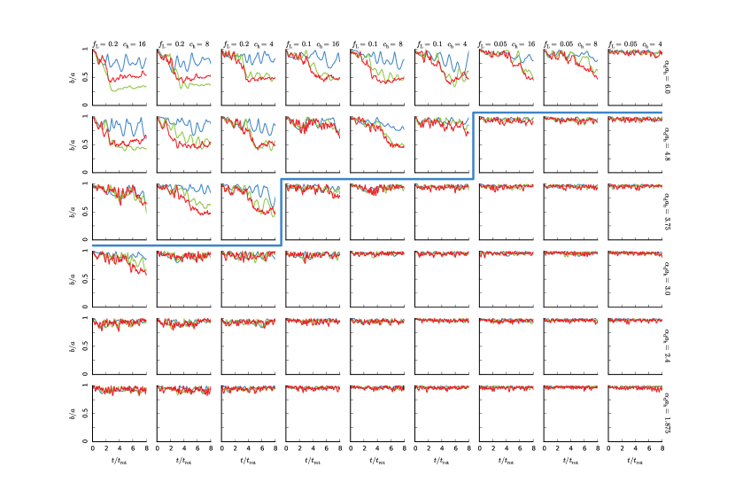
Figure 23: Stability tests for bulge/disc/halo galaxy models. The layout is similar to Fig. 2 but adds another row of models with $\alpha_{\mathrm{d}}a_{\mathrm{h}}=6.0$ at the top; the heavy blue line is the same approximate stability boundary shown previously. Red, green, and blue curves show $b/a$ ratios for the inner $25$ percent, $50$ percent and $75$ percent of each disc, respectively.

Simulations were run using a hierarchical $N$-body code. An opening angle of $\theta=0.8$, together with quadrapole moments, yields accelerations with median errors $\delta\mathbf{a}/|\mathbf{a}|\lesssim 0.0006$. Trajectories were integrated using a time-centred leap-frog, with a time-step $\Delta t=1/1024$ for all bodies.

APPENDIX B: STABILITY TESTS

Galaxy models with massive, largely self-gravitating discs tend to be dynamically unstable to bar formation. In the context of the present study, instability results when the parameter $\alpha_{\mathrm{d}}a_{\mathrm{h}}$ exceeds a critical value which depends on the chosen values of $f_{\mathrm{L}}$ and $c_{\mathrm{h}}$. The rationale for excluding unstable models from these experiments is complex. Violently unstable initial models are unrealistic. There’s no plausible way that nature could assemble such configurations, since a bar would develop long before the entire mass of the galaxy was in place; presumably the bar would then heat the disc, producing a near-equilibrium configuration. Starting with a violently unstable system and allowing it to evolve is unlikely to produce a similar configuration. Mildly unstable initial conditions are more plausible, provided the bars have enough time to develop and approach equilibrium before the galaxies interact. Tidal interactions of barred galaxies are certainly interesting (e.g., Gerin, Combes, & Athanassoula, 1990), but introduce yet another parameter – the phase angle of the bar at the time of pericentre – into a problem which already has a daunting number of parameters. For practical reasons, such encounters are excluded from the present study.

To determine the stability boundary in Fig. 2, individual galaxy models were set up following the procedure in § 2.1.2 and run in isolation. Visually reviewing the resulting array of simulations proved quite exhausting, so a simple procedure was developed to quantify the (in)stability of the models. At the start of each simulation, disc bodies are sorted by orbital radius. This makes it easy to track the Lagrangian volumes corresponding to the inner $25$ percent, $50$ percent and $75$ percent of each disc. At each time step, the moment-of-inertia tensor for each of these volumes is computed, its eigenvalues $q_{1}$, $q_{2}$ are determined, and the axial ratio $b/a=\sqrt{\min(q_{1},q_{2})/\max(q_{1},q_{2})}$ is evaluated. These axial ratios are plotted as functions of time in Fig. 23. Each model was run to time $t=8t_{\mathrm{rot}}$, where $t_{\mathrm{rot}}$ is the rotation period at $R=2\alpha_{\mathrm{d}}^{-1}$, to insure bars have time to develop.

Models shown in the bottom rows of Fig. 23 maintain axial ratios $b/a\simeq 1$ for the duration of the simulations. These discs exhibit transitory spiral features, but no lasting bisymmetric patterns emerge. On the other hand, disc-dominated models, such as those in the upper-left region of this diagram, are violently unstable; within a few $t_{\mathrm{rot}}$ they develop strong bars within the inner $50$ percent of their discs. For the purposes of the present study, I adopted the stability boundary shown in Figs. 2 and 23, fixing the maximum value of $\alpha_{\mathrm{d}}a_{\mathrm{h}}$ for a given value of $f_{\mathrm{L}}$ independent of $c_{\mathrm{h}}$. This choice is somewhat arbitrary; it included the models with $(f_{\mathrm{L}},c_{\mathrm{h}},\alpha_{\mathrm{d}}a_{\mathrm{h}})=(0.2,16,3.0)$ and $(0.1,16,3.75)$, which both seem to be developing small bars at later times, and excluded the model with $(f_{\mathrm{L}},c_{\mathrm{h}},\alpha_{\mathrm{d}}a_{\mathrm{h}})=(0.05,4,6.0)$, which appears to be stable. However, the regular structure of the adopted boundary makes the organization and presentation of the experiments much more straightforward.

While a general stability criterion is not easy to define, stable disc models typically satisfy $\epsilon_{\mathrm{m}}\gtrsim\epsilon_{\mathrm{m,crit}}$, where

$$\epsilon_{\mathrm{m}}=\frac{v_{\mathrm{max}}}{\sqrt{GM_{\mathrm{d}}\alpha_{\mathrm{d}}}}\,,$$ (15)

$v_{\mathrm{max}}$ is the maximum rotation velocity of the model, and the stability threshold is in the range $\epsilon_{\mathrm{m,crit}}\simeq 1.1$ (Efstathiou, Lake, & Negroponte, 1982) to $\epsilon_{\mathrm{m,crit}}\simeq 0.75$ (Syer, Mao, & Mo, 1998). Fig. 24 plots the relationship between $\epsilon_{\mathrm{m}}$ and the time-averaged value of the $b/a$ ratio for the inner quartile of each disc; the average is taken over times $6\leq t/t_{\mathrm{rot}}\leq 8$. Open symbols represent a parallel set of models without bulges; in these models, disc masses are increased by factors of $1/3$, so as to obtain the same $f_{\mathrm{L}}$, and all other parameters are left unchanged. It appears that $\epsilon_{\mathrm{m}}$ provides a approximate criterion for stability, but doesn’t always characterize marginally stable discs correctly. In particular, bulges exert a stabilizing influence which is not completely reflected in the value of $\epsilon_{\mathrm{m}}$.

Figure 24: Scatter plot of the axial ratio for the inner disc quartile, $(\overline{b/a})_{\mathrm{25}}$, time-averaged for $6\leq t/t_{\mathrm{rot}}\leq 8$, versus the stability index $\epsilon_{\mathrm{m}}$. Open squares are models without bulges (i.e., the disc mass is increased by a factor of $1/3$). Filled circles are models below the stability boundary in Fig. 2, while filled squares are above the stability boundary. The $\alpha_{\mathrm{d}}a_{\mathrm{h}}$ values represented range from $6.0$ to $1.2$.

References

- (1)
- (2)
- Aarseth (1963) Aarseth, S.J. 1963, MNRAS, 126, 223–255
- Armus et al. (2009) Armus, L. et al. 2009, PASP, 121, 559–576
- Arp (1966) Arp, H. 1966, ApJS, 14, 1–20
- Barnes (1987) Barnes, J.E. 1987, in S.M. Faber, ed., Nearly Normal Galaxies. Springer, New York, p. 154–159
- Barnes (1988) Barnes, J.E. 1988, ApJ, 331, 699–717
- Barnes (1992) Barnes, J.E. 1992, ApJ, 393, 484–507
- Barnes (1999) Barnes, J.E. 1999, in J.E. Barnes, D.B. Sanders, eds, Proc. IAU Symp. 186, Galaxy Interactions at Low and High Redshift. Kluwer, Dordrecht, p. 137–144
- Barnes (2012) Barnes, J.E. 2012, MNRAS, 425, 1104–1120
- Barnes & Hibbard (2009) Barnes, J.E., Hibbard, J.E. 2009, AJ, 137, 3071–3090
- Bekenstein & Milgrom (1984) Bekenstein, J., Milgrom, M. 1984, ApJ, 286, 7–14
- Bett et al. (2007) Bett, P., Eke, V., Frenk, C.S., Jenkins, A., Helly, J., Navarro, J. 2007, MNRAS, 376, 215–232
- Blumenthal et al. (1986) Blumenthal, G.R., Faber, S.M., Flores, R., Primack, J.R. 1986, ApJ, 301, 27–34
- Brook et al. (2011) Brook, C.B., et al. 2011, MNRAS, 415, 1051–1060
- Côté, Carignan, & Freeman (2000) Côté, S., Carignan, C., Freeman, K.C. 2000, AJ, 120, 3027–3059
- Casertano & van Gorkom (1991) Casertano, S., van Gorkom, J.H. 1991, AJ, 101, 1231–1241
- D’Onghia et al. (2010) D’Onghia, E., Vogelsberger, M., Faucher-Giguere, C.-A., Hernquist, L. 2010, ApJ, 725, 353–368
- Dalcanton, Spergel, & Summers (1997) Dalcanton, J.J., Spergel, D.N., Summers, F.J. 1997, ApJ, 482, 659–676
- de Blok, McGaugh, & Rubin (2001) de Blok, W.J.G., McGaugh, S.S., Rubin, V.C. 2001, AJ, 122, 2396–2427
- de Blok, Bosma, & McGaugh (2003) de Blok, W.J.G., Bosma, A., McGaugh, S. 2003, MNRAS, 340, 657–678
- de Blok et al. (2008) de Blok, W.J.G., Walter, F., Brinks, E., Trachternach, C., Oh, S.-H., & Kennicutt, R.C. Jr. 2008, AJ, 136, 2648–2719
- Dubinski, Mihos, & Hernquist (1996) Dubinski, J., Mihos, J.C., Hernquist, L. 1996, ApJ, 462, 576–593
- Dubinski, Mihos, & Hernquist (1999) Dubinski, J., Mihos, J.C., Hernquist, L. 1999, ApJ, 526, 607–622
- Dutton et al. (2011) Dutton, A.A., et al. 2011, MNRAS, 417, 1621–1642
- Efstathiou, Lake, & Negroponte (1982) Efstathiou, G., Lake, G., Negroponte, J. 1982, MNRAS, 199, 1069–1088
- Fall (1983) Fall, S.M. 1983, in E. Athanassoula, ed., Internal Kinematics and Dynamics of Galaxies. D. Reidel, Dordrecht, p. 391–398
- Fall & Efstathiou (1980) Fall, S.M., Efstathiou, G. 1980, MNRAS, 193, 189–206
- Farouki & Shapiro (1982) Farouki, R.T., Shapiro, S.L. 1982, ApJ, 259, 103–115
- Freeman (1999) Freeman, K.C. 1999, in J.I. Davies, C. Impey, S. Phillipps, eds, ASP Conf. Ser. Vol. 170, The Low Surface Brightness Universe. Astron. Soc. Pac., San Francisco, p. 3–8
- Genel et al. (2015) Genel S., Fall S.M., Hernquist L., Vogelsberger M., Snyder G.F., Rodriguez-Gomez V., Sijacki D., Springel V., 2015, ApJL, 804, L40
- Gerin, Combes, & Athanassoula (1990) Gerin, M., Combes, F., Athanassoula, E. 1990, A&A, 230, 37–54
- Giodini et al. (2009) Giodini, S., et al. 2009, ApJ, 703, 982–993
- Gnedin et al. (2004) Gnedin, O.Y., Kravtsov, A.V., Klypin, A.A., Nagai, D. 2004, ApJ, 616, 16–26
- Governato et al. (2012) Governato, F., et al. 2012, MNRAS, 422, 1231–1240
- Hernquist (1990) Hernquist, L. 1990, ApJ, 356, 359–364
- Hinshaw et al. (2013) Hinshaw, G., et al. 2013, ApJS, 208, 19
- Hoyle (1949) Hoyle, F. 1949, in J.M. Burgers and H.C. van de Hulst, eds, Problems of Cosmological Aerodynamics. Internat. Union Theoret. Appl. Mech. & Internat. Astr. Union, p. 195
- Jaffe (1983) Jaffe, W. 1983, MNRAS, 202, 995–999
- Katz & Gunn (1991) Katz, N., Gunn, J.E. 1991, ApJ, 377, 365–381
- Kereš et al. (2012) Kereš, D., Vogelsberger, M., Sijacki, D., Springel, V., Hernquist, L. 2012, MNRAS, 425, 2027–2048
- Lotz et al. (2011) Lotz, J.M., Jonsson, P., Cox, T.J., Croton, D., Primack, J.R., Somerville, R.S., Stewart, K. 2011, ApJ, 742, 103
- Lynds & Toomre (1976) Lynds, R., Toomre, A. 1976, ApJ, 209, 382–388
- Ludlow et al. (2014) Ludlow, A.D., Navarro, J.F., Angulo, R.E., Boylan-Kolchin, M., Springel, V., Frenk, C., & White, S.D.M. 2014, MNRAS, 441, 378–388
- Martin et al. (2012) Martin, C.L., Shapley, A.E., Coil, A.L., Kornei, K.A., Bundy, K., Weiner, B.J., Noeske, K.G., & Schiminovich, D. 2012, ApJ, 760, 127
- McGaugh et al. (2000) McGaugh, S.S., Schombert, J.M., Bothun, G.D., de Blok, W.J.G. 2000, ApJL, 533, L99–L102
- Mihos, Dubinski, & Hernquist (1998) Mihos, J.C., Dubinski, J., Hernquist, L. 1998, ApJ, 494, 183–193
- Mo, Mao, & White (1998) Mo, H.J., Mao, S., White, S.D.M. 1998, MNRAS, 295, 319–336
- Mo, van den Bosch, & White (2010) Mo, H., van den Bosch, F.C., White, S. 2010, Galaxy Formation and Evolution, Cambridge University Press, Cambridge, UK
- Navarro, Frenk, & White (1996) Navarro, J.F., Frenk, C.S., White, S.D.M. 1996, ApJ, 462, 563–575
- Navarro, Frenk, & White (1997) Navarro, J.F., Frenk, C.S., White, S.D.M. 1997, ApJ, 490, 493–508
- Peebles (1969) Peebles, P. J. E. 1969, ApJ, 155, 393–401
- Pettini et al. (2001) Pettini, M., Shapley, A.E., Steidel, C.C., Cuby, J.-G., Dickinson, M., Moorwood, A.F.M., Adelberger, K.L., & Giavalisco, M. 2001, ApJ, 554, 981–1000
- Planck Collaboration et al. (2015) Planck Collaboration et al. 2015, preprint, (arXiv:1502.01589)
- Plummer (1911) Plummer, H.C. 1911, MNRAS, 71, 460–470
- Romanowsky & Fall (2012) Romanowsky, A.J., Fall, S.M. 2012, ApJS, 203, 17
- Sanders & McGaugh (2002) Sanders, R.H., McGaugh, S.S. 2002, ARA&A, 40, 263–317
- Schombert, Wallin, & Struck-Marcell (1990) Schombert, J.M., Wallin, J.F., Struck-Marcell, C. 1990, AJ, 99, 497–529
- Scoville et al. (1998) Scoville, N.Z., et al. 1998, ApJL, 492, L107–L110
- Schweizer (1982) Schweizer, F. 1982, ApJ, 252, 455–460
- Sellwood (1999) Sellwood, J.A. 1999, in D.R. Merritt, M. Valluri, J.A. Sellwood, eds, ASP Conf. Ser. Vol. 182, Galaxy Dynamics. Astron. Soc. Pac., San Francisco, p. 351–364
- Sellwood & McGaugh (2005) Sellwood, J.A., McGaugh, S.S. 2005, ApJ, 634, 70–76
- Smith et al. (2010) Smith, B.J., Giroux, M.L., Struck, C., Hancock, M. 2010, AJ, 139, 1212–1241
- Springel & White (1999) Springel, V., White, S.D.M. 1999, MNRAS, 307, 162–178
- Steidel et al. (2010) Steidel, C.C., Erb, D.K., Shapley, A.E., Pettini, M., Reddy, N., Bogosavljević, M., Rudie, G.C., & Rakic, O. 2010, ApJ, 717, 289–322
- Stewart et al. (2013) Stewart, K.R., Brooks, A.M., Bullock, J.S., Maller, A.H., Diemand, J., Wadsley, J., Moustakas, L.A. 2013, ApJ, 769, 74
- Swaters et al. (2003) Swaters, R.A., Madore, B.F., van den Bosch, F.C., Balcells, M. 2003, ApJ, 583, 732–751
- Syer, Mao, & Mo (1998) Syer, D., Mao, S., Mo, H.J. 1998, preprint, (arXiv:astro-ph/9711160)
- Tecza et al. (2000) Tecza, M., Genzel, R., Tacconi, L.J., Anders, S., Tacconi-Garman, L.E., Thatte, N. 2000, ApJ, 537, 178–190
- Theys & Spiegel (1977) Theys, J.C., Spiegel, E.A. 1977, ApJ, 212, 616–619
- Tiret & Combes (2008) Tiret, O., Combes, F. 2008, in Jose G. Funes, S.J., and Enrico Maria Corsini, eds, ASP Conf. Ser. Vol. 396, Formation and Evolution of Galaxy Discs, Astron. Soc. Pac., San Francisco, p. 259–262
- Tissera et al. (2010) Tissera, P.B., White, S.D.M., Pedrosa, S., Scannapieco, C. 2010, MNRAS, 406, 922–935
- Toomre & Toomre (1972) Toomre, A., Toomre, J. 1972, ApJ, 178, 623–666
- Torrey et al. (2012) Torrey, P., Vogelsberger, M., Sijacki, D., Springel, V., Hernquist, L. 2012, MNRAS, 427, 2224–2238
- Tsatsi et al. (2015) Tsatsi, A., Macciò, A.V., van de Ven, G., Moster, B.P. 2015, ApJL, 802, L3
- White (1978) White, S.D.M. 1978, MNRAS, 184, 185–203
- Wilson & Kalnajs (2002) Wilson, G., Kalnajs, A. 2002, in G.S. Da Costa and Helmut Jerjen, eds, ASP Conf. Ser. Vol. 273, The Dynamics, Structure & History of Galaxies: A Workshop in Honour of Professor Ken Freeman, Astron. Soc. Pac., San Francisco, p. 363–367
- Young (1980) Young, P. 1980, ApJ, 242, 1232–1237
- Verheijen (2001) Verheijen, M.A.W. 2001, ApJ, 563, 694–715
- Zaritsky et al. (2014) Zaritsky, D., et al. 2014, AJ, 147, 134
- Zhao et al. (2003) Zhao, D.H., Jing, Y.P., Mo, H.J., Böumlrner, G. 2003, ApJL, 597, L9–L12