EUV Spectra of Solar Flares from the EUV Spectroheliograph SPIRIT aboard CORONAS-F satellite

Abstract

We present detailed EUV spectra of 4 large solar flares: M5.6, X1.3, X3.4, and X17 classes in the spectral ranges 176–207 Å and 280–330 Å. These spectra were obtained by the slitless spectroheliograph SPIRIT aboard the CORONAS-F satellite. To our knowledge these are the first detailed EUV spectra of large flares obtained with spectral resolution of $\sim 0.1$ Å. We performed a comprehensive analysis of the obtained spectra and provide identification of the observed spectral lines. The identification was performed based on the calculation of synthetic spectra (CHIANTI database was used), with simultaneous calculations of DEM and density of the emitting plasma. More than 50 intense lines are present in the spectra that correspond to a temperature range of $T=0.5-16$ MK; most of the lines belong to Fe, Ni, Ca, Mg, Si ions. In all the considered flares intense hot lines from Ca XVII, Ca XVIII, Fe XX, Fe XXII, and Fe XXIV are observed. The calculated DEMs have a peak at $T\sim 10$ MK. The densities were determined using Fe XI–Fe XIII lines and averaged $6.5\times 10^{9}$ cm^-3. We also discuss the identification, accuracy and major discrepancies of the spectral line intensity prediction.

1 Introduction

The extreme ultra-violet (EUV) emissions of the solar corona have been studied since the beginning of the space era due to the rich informational content of the registered spectra. Analysis of such spectra allows the determination of various plasma characteristics, such as temperature and density, and provides information about dynamic processes that take place in the solar corona. In addition, the EUV spectra of different coronal phenomena have become a subject of interest in a number of different areas such as atomic physics, astrophysics and physics of plasma.

Numerous spectroscopic observations have been carried out using spectroscopic instruments of different types: slit spectroghraphs with high spatial resolution, such as SERTS (Neupert et al., 1992), CDS/SOHO (Harrison et al., 1995), EIS/Hinode (Culhane et al., 2007); spectroheliographs with imaging capabilities, such as S082A/Skylab (Tousey et al., 1977), SPIRIT/CORONAS-F (Zhitnik et al., 2002); and full-Sun spectrographs, which obtain spectra from the whole solar disk, such as those on the Aerobee rocket (Malinovsky & Heroux, 1973) or EVE/SDO (Woods et al., 2012).

Data obtained in these experiments have been used for various goals such as for development of atlases of spectral lines, validation of atomic data, measurement of temperature and density of the emitting plasma in different structures, determination of presence of up- or downflows etc. Among the structures that were studied, there are quiet sun regions (Brosius et al., 1996), active regions (AR) cores (Tripathi et al., 2011), off-limb AR plasma (O’Dwyer et al., 2011), AR mosses (Tripathi et al., 2010), coronal streamers (Parenti et al., 2003), bright points (Ugarte-Urra et al., 2005) and others.

Whereas solar flares have also been observed by spectrographs, obtaining EUV spectra of solar flares is not so common. The first systematic analysis of EUV flaring spectra was presented by Dere (1978). The author analyzed more than 50 photographic plates from the S082A spectroheliograph on Skylab and constructed a catalog of spectral lines in the range 171–630 Å. The catalog included relative intensities of more than 200 spectral lines.

Systematic studies of EUV spectra of solar flares have been continued on subsequent satellites: SOHO (launched in 1995), Hinode (launched in 2006), and SDO (launched in 2010). The CDS spectrograph aboard the SOHO satellite registered several large solar flares during their decay phases. The first analysis of a CDS flare was made by Czaykowska et al. (1999). The authors analysed intensities of spectral lines during the decay phase of a M6.8 flare and determined density and temperature of post-flare loops. Del Zanna et al. (2006) also performed analysis of spectra of a X17 flare during the decay phase. The authors studied Doppler shifts and found them to be consistent with those, predicted by a simple hydrodynamics model. It is worth noting that due to the telemetry constraints of CDS, all these flares were observed in fast-rastering regime in only 6 narrow spectral windows, covering only a small portion of the wide spectral ranges 308–381 and 513–633 Å of CDS.

The EIS spectrograph aboard the Hinode satellite used an improved optical layout with high efficiency EUV optics and detectors. Therefore, EIS has superb spectral, spatial and temporal resolution as well as higher telemetry volumes, which allow spectra to be investigated with much higher details, such as a wider set of spectral lines, higher cadence, and higher spatial resolution. EIS has observed a large span of flares, starting from small B2 class (Del Zanna et al., 2011) to large M1.8 (Doschek et al., 2013). However, despite all its advantages, EIS usually observes flares in coarse rastering regime. This fact limits the number of spectral lines observed in a flarer; for example Watanabe et al. (2010) used only 17 lines for plasma diagnostics from the whole spectral range 170–210 and 250–290 Å. There is a case when EIS has registered a full CCD flare spectrum (Doschek et al., 2013); however, the authors focused on Doppler shift analysis and used only 17 out of 500 lines registered by EIS.

The EVE spectrometer aboard SDO builds whole-Sun spectra in the range 10–1050 Å. It has moderate spectral resolution of 1 Å  but operates with an unprecedented 10 seconds cadence and almost 100 % duty cycle. There are two main difficulties in analysis of the EVE spectra: it has no spatial resolution — flare spectrum is mixed with the spectrum from the rest of the Sun, and due to moderate spectral resolution of EVE most of the lines are blended. Despite these obstacles EVE is widely used in solar investigations: for study of thermal evolution of flaring plasma (Chamberlin et al., 2012), Doppler shifts study (Hudson et al., 2011), and high temperature plasma electron density diagnostics (Milligan et al., 2012).

Without diminishing the importance of the information obtained in these experiments, it should be noted that a small number of EUV spectra of solar flares have been registered so far, and published catalogs of spectral lines are limited.

In this paper we take advantage of the SPIRIT EUV spectroheliograph and perform a comprehensive analysis of EUV spectra of four large solar flares. The flares of M5.6, X1.3, X3.4 and X17 classes have been observed by a slitless EUV spectroheliograph SPIRIT aboard CORONAS-F satellite. The spectroheliograph operated in two wavelength ranges 176–207 and 280–330 Å and had a spectral resolution of 0.1 Å. We perform an absolute calibration of SPIRIT spectral fluxes using simultaneous EIT/SOHO images. In order to identify the obtained spectra we use an original approach, based on calculation of synthetic spectra and its subsequent modification to match the observational data. Simultaneously, we calculate DEM and $n_{e}$ of the emitting plasma and repeat iteratively the whole procedure of identification several times.

We provide identification of more than 50 spectral lines in each spectral band for each flare. In addition to spectral line intensities, we calculate the DEM and plasma density for each flare. The obtained information can be used not only for modelling of spectral fluxes in different EUV spectral bands and for refinement of the atomic data, but also for studying flares themselves and validating models for flare plasma evolution.

The obtained spectra, synthetic spectra, DEMs, and proposed IDL software are available at http://xras.lebedev.ru/SPIRIT/ or on request from S. Shestov.

2 Observations

The SPIRIT complex of instrumentation was launched aboard the CORONAS-F satellite (Oraevsky & Sobelman, 2002) on 31st July 2001 from Plesetsk cosmodrome, northern Russia. The satellite was placed on a near-polar orbit with an inclination of $82^{\circ}$ and a perigee of 500 km. The satellite carried 12 scientific instruments for the measurement of both particle and electromagnetic emission of the Sun. The SPIRIT instrumentation was developed in the Lebedev Physical Institute of the Russian Academy of Sciences and consisted of telescopic and spectroheliographic channels for observation of the solar corona in different soft X-ray and EUV spectral bands (Zhitnik et al., 2002).

The EUV spectroheliograph SPIRIT consisted of two similar independent spectral channels: V190 channel for 176–207 Å range, and U304 channel for 280–330 Å range. Both channels were built using a slitless optical scheme (see Figure 1). The solar EUV emission enters through an entrance filter, falls on a diffraction grating (with a grazing angle $\varphi\sim 1.5^{\circ}$). Diffracted radiation is focused on a detector by a mirror with multilayer coating.

The slitless optical scheme observes full-Sun FOV on the detector, which allowed us to obtain as many as 30 spectroheliograms with large solar flares during 4.5 years of the satellite’s lifetime.

Figure 1: Optical scheme of EUV slitless spectroheliograph SPIRIT aboard CORONAS-F satellite.

For the analysis, we have selected the following flares: M5.6 observed on 2001 September 16, X3.4 observed on 2001 December 28, X1.3 observed on 2004 July 16, and X17 flare observed on 2005 September 7. All these flares are long duration events (LDE), cover a broad range of flare intensity and have been registered in different phases of their decay. The X-ray lightcurves of the flares measured by GOES are shown in Figure 2. Each SPIRIT spectroheliogram was obtained in a single exposure (the exposures are denoted by vertical lines in the Figure 2). The exposure times for the M5.6 and X3.4 flares were 37 seconds, and 150 seconds for the X1.3 and X17 flares. Some details of the analyzed flares are given in the Table 1.

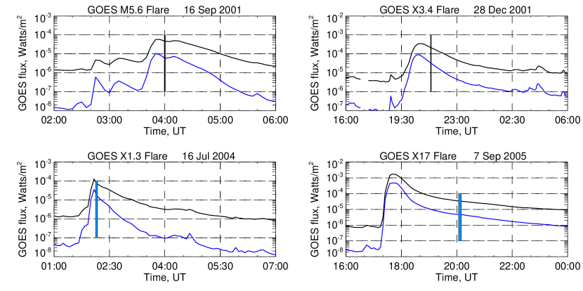
Figure 2: GOES X-ray lightcurves of the 4 flares. The vertical lines highlight the time when the SPIRIT spectroheliograms were obtained.

Table 1: Flares class, peak time, active regions

GOES class	Date	GOES peak time, UT	SPIRIT obs. start, UT	NOAA AR	type, tdecay
M5.6	2001-09-16	$\sim$ 03:50	03:59:36	9608	LDE, 1 h 30 min
X1.3	2004-07-16	$\sim$ 02:05	02:07:54	10649	LDE, $\sim 7$ h
X3.4	2001-12-28	$\sim$ 20:40	21:21:45	9767	LDE, 2 h 40 min
X17	2005-09-07	$\sim$ 17:40	20:04:22	10808	LDE, 5 h 50 min

3 Data analysis

3.1 Interpretation of the SPIRIT spectroheliograms

In a slitless scheme a set of monochromatic solar images (each image in a particular spectral line) is obtained on the detector, shifted along the dispersion axis. A small grazing incidence $\varphi\sim 1.5^{\circ}$ results in a contraction of solar images along the dispersion axis.

Examples of the SPIRIT spectroheliograms are given in the middle panels of Figure 3 and 4. The X1.3 flare (Figure 3) appears as the bright horizontal line in the center in the U304 channel. The X17 flare (Figure 4) appears as a brightening in the upper part of the solar disk in the V190 channel. On the bottom panels of both Figures, directly extracted (“raw”) scans are given: scan1 corresponds to the flare, and scan2 corresponds to arbitrary quite Sun area. These raw scans are rows from respective images-arrays with a roughly assigned linear wavelength scale. On the top panels of both Figures simultaneous EUV images are given: EIT 195 Å (Figure 4) and SPIRIT 175 Å (Figure 3; no simultaneous EIT image was available).

Comparison of the spectroheliograms and the extracted spectra shows that emission of “cold” coronal lines (like Si IX, Mg VIII, Fe XI, Fe XII with $T_{max}\sim 1-2$ MK) originates from the whole solar disk, but due to contraction these monochromatic full-disk images look like ellipses. Emission of “hot” coronal lines (Ca XVII, Ca XVIII, Fe XX, Fe XXII, Fe XXIV with $T_{max}>6$ MK ) is produced mainly in flaring regions, which correspond to bright points in the spectroheliograms.

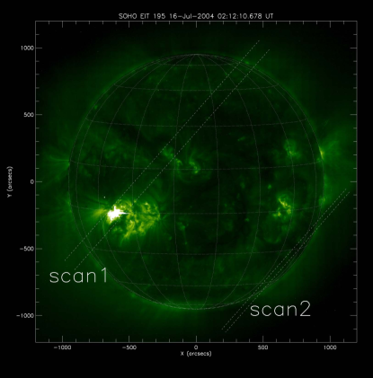
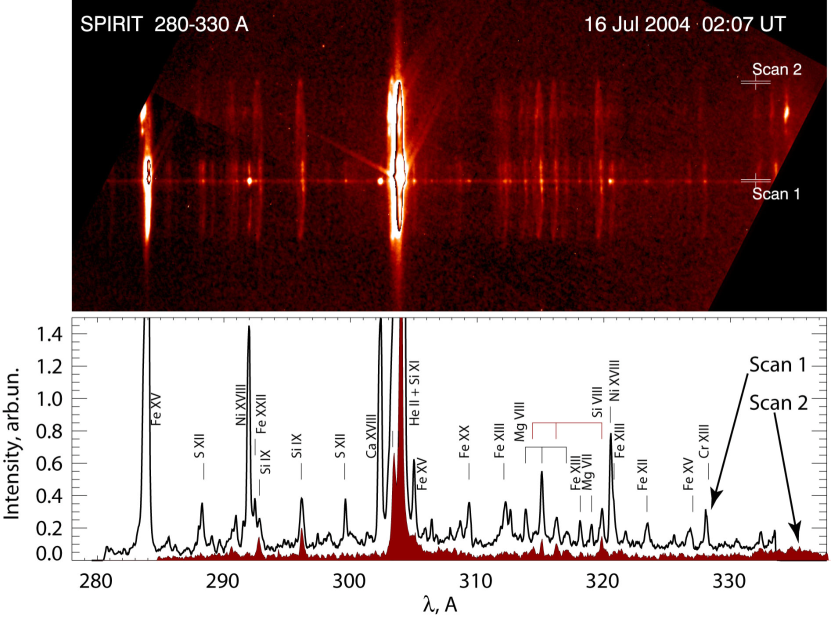
Figure 3: SPIRIT spectroheliogram for the 280–330 Å range. Top panel: corresponding EIT 195 Å image. Middle panel: the spectroheliogram registered on 2004 July 16; bottom panel: spectra of two regions — flaring (scan1 — X1.3 class flare) and arbitrary QS (scan2). On the spectroheliogram each ellipse is a monochromatic solar disk image (in a particular spectral line) contracted along the dispersion axis.

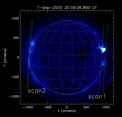
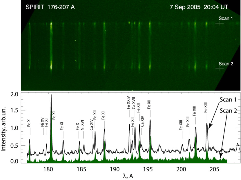
Figure 4: SPIRIT spectroheliogram for the 176–207 Å range. Top panel: corresponding SPIRIT 175 Å telescope image (no EIT images were available on that day). Middle panel: the spectroheliogram registered on 2005 September 7; bottom panel: spectra of two regions — flaring (scan1 — X17 class flare) and arbitrary QS (scan2). On the spectroheliogram each ellipse is a monochromatic solar disk image (in a particular spectral line) contracted along the dispersion axis.

The interpretation of the spectroheliograms involves the following steps: a) obtaining spectra of a particular region and determining the wavelength scale; b) subtracting background from the spectra; c) identifying spectral lines with a subsequent analysis of spectral data.

For obtaining spectra from the spectroheliograms we have developed IDL software, which implements a geometrical model of the spectroheliograph. According to the model, for a particular point source the position on the CCD-detector is calculated using its solar coordinates, wavelengths and several parameters (such as direction to the solar center, groove density of the diffraction grating, focal length and direction of the focusing mirror, relative position of the CCD-detector etc.). The geometrical model automatically takes into account contraction of solar disk images and non-linear wavelength scale across the CCD-detector. Thus, to obtain spectra of a particular region and calculate the wavelength scale for it, one has only to point to the region on the solar disk. The accuracy of the obtained wavelength scale is comparable to the spectral size of 1 pixel ($\sim 0.04$ Å).

For background subtraction we used a procedure similar to that of Thomas & Neupert (1994) — we interpolated values outside spectral lines and subtracted the interpolation from spectra.

Before the identification we also carefully removed strong Si XI ($\lambda=303.33$ Å) and He II (doublet $\lambda=303.78+.79$ Å) blend from spectra. This reveals the spectral lines of Ca XVIII, Ni XIV, Fe XV ($\lambda\approx 302$ Å) and Fe XVII, Fe XV ($\lambda\approx 305$ Å), which lie on the wings of the Si XI/He II blend. These lines are well distinguished on the wings of the blend (see Figure 3); therefore, we remove the wings of the blend by interpolating the values outside the lines and manually zero out the core of the blend.

In order to identify the observational spectrum and measure intensities of separate spectral lines, we produced a synthetic spectrum, which fits the observational data. To produce a synthetic spectrum we use transitions and wavelengths from CHIANTI (CHIANTI v.6 was used, Dere et al. (1997, 2009)), set the line widths $\sigma$ in accordance with the instrument FWHM ($\sigma=-0.201+1.43\cdot 10^{-3}\cdot\lambda$ [Å] for the V190 channel and $\sigma=0.1$ [Å] for the U304 channel), and vary intensities to match the observational data. However, straightforward fitting is not possible due to the relatively low spectral resolution of SPIRIT — $\sigma\sim 0.1$ Å and blending of most of the lines.

We overcome this obstacle using an iterative procedure (see Figure 5), which consists of the initial step:

• Measurement of intensities of a small number of spectral lines and calculation of plasma parameters — DEM and $n_{e}$ (see Shestov et al. (2009, 2010));

and further (iterative) steps:

• Calculation of the synthetic spectra;

• Automated adjustment of spectral line intensities to match the observational data. During the adjustment, the ratio of the blended lines is kept constant;

• Manual adjustment of intensities of particular spectral lines. Using the DEM and $n_{e}$ analysis data we adjust intensities of blended lines to reach a better agreement with theory (reducing $\chi^{2}$ in DEM reconstruction and compliance with other lines in L-function analysis — see below);

• Calculation of DEM and $n_{e}$.

The larger number of spectral lines, used for analysis during iterative steps, almost completely eliminates errors due to possible misidentification or other errors. The iterative procedure turned out to be fast and stable — after the second step there are no considerable changes in DEMs and synthetic spectra. So, in our approach plasma diagnostic was an essential part of the line identification — we used plasma parameters to resolve blended lines.

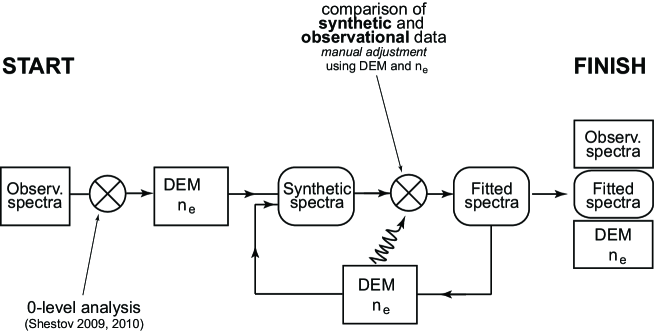
Figure 5: Procedure for spectra analysis.

For the calculation of synthetic spectra we used standard CHIANTI procedures ch_synthetic and make_chianti_spec, coronal abundances sun_coronal.abund and mazzotta_etal.ioneq ionization equilibrium.

For the DEM reconstruction we used a Genetic Algorithm (GA) (Siarkowski et al., 2008). The algorithm is based on ideas of biological evolution and natural selection. It starts from randomly chosen initial populations of different DEMs and produces a new generation of DEMs by crossover and mutations. The procedure stops when a local $\chi^{2}$ minimum is found. The peculiar feature of the method is that since it is based on a random evolution, different runs of the procedure on a single data set give different (but similar) results. The discrepancy among different runs directly shows the confidence of the DEM reconstruction.

For the DEM analysis we carefully chose 46 spectral lines (Table 3.1) — almost all strong spectral lines, observed by SPIRIT. The exceptions are Fe XV 284.16 Å and the Si XI/He II blend with $\lambda\sim 304$ Å. Both these lines are very intense, which is likely to cause saturation of the SPIRIT detector. Also, the observed intensity of the Fe XV line shows systematic discrepancy with other Fe XV lines (we will discuss possible reasons later). Nevertheless, the spectral lines analysed cover a wide temperature range — from $T_{max}\sim 1$ MK (Mg VIII) to $T_{max}\sim 16$ MK (Fe XXIV). Using of a large number of lines almost completely eliminates the sensitivity of the reconstructed DEM to the intensity of a particular line, improving reliability of the reconstruction.

Table 2: List of spectral lines used in the DEM reconstruction.

N	Ion	$\lambda$, Å	$\log T_{m}$, K	N	Ion	$\lambda$, Å	$\log T_{m}$, K	N	Ion	$\lambda$, Å	$\log T_{m}$, K
1	Fe XI	180.41	6.2	17	Fe XIII	196.54	6.3	33	Fe XIII	312.11	6.3
2	Fe XI	182.17	6.2	18	Fe XII	196.64	6.3	34	Fe XII	312.25	6.3
3	Fe X	184.54	6.2	19	Fe XIII	200.02	6.3	35	Mg VIII	313.74	6.0
4	Ni XVI	185.23	6.4	20	Fe XIII	202.04	6.3	36	Si VIII	314.36	6.1
5	Ca XIV	186.61	6.6	21	Fe XIII	203.83	6.3	37	Mg VIII	315.02	6.0
6	Fe XII	186.89	6.3	22	S XI	285.82	6.3	38	Si VIII	316.22	6.1
7	Fe XXI	187.93	7.1	23	Ni XVI	288.17	6.4	39	Mg VIII	317.03	6.0
8	Fe XI	188.23	6.2	24	Ni XVIII	291.98	6.8	40	Fe XIII	318.13	6.3
9	Fe XI	188.30	6.2	25	Fe XXII	292.46	7.1	41	Mg VII	319.03	5.8
10	Fe XXIV	192.03	7.2	26	Si IX	292.76	6.2	42	Si VIII	319.84	6.1
11	Fe XII	192.39	6.3	27	Si IX	296.11	6.2	43	Ni XVIII	320.57	6.8
12	Fe XI	192.83	6.2	28	S XII	299.54	6.3	44	Fe XIII	320.81	6.3
13	Ca XVII	192.85	6.8	29	Ca XVIII	302.19	7.0	45	Fe XII	323.41	6.3
14	Fe XII	193.51	6.3	30	Fe XV	302.33	6.3	46	Fe XVII	323.65	6.8
15	Ca XIV	193.87	6.6	31	Fe XV	304.89	6.3	47	Fe XV	327.03	6.3
16	Fe XII	195.12	6.3	32	Fe XX	309.29	7.0

Electron density $n_{e}$ was obtained using a modified L-function analysis (Landi & Landini, 1998). According to the original method proposed by the authors, L-functions of all spectral lines of a particular ion should intersect at a single point, corresponding to the density of the emitting plasma. The L-function of a spectral line is defined as a ratio of measured intensity over the contribution function $G(T_{o},n_{e})$, plotted as a function of density. We slightly simplify the definition of L-function by using $T_{max}$ instead of $T_{o}$ (specially computed temperature) and plot the L-functions for major lines of the Fe XI, Fe XII, Fe XIII, Fe XV, Mg VIII, and Ni XVI ions.

3.2 Absolute calibration of SPIRIT fluxes

No absolute ground calibration was carried out before the launch of the SPIRIT. Lack of calibration cripples spectroheliograph diagnostic capabilities. However, the spectral ranges of the SPIRIT V190 and U304 channels overlap with spectral responses of the EIT 195 Å and 304 Å channels, and it is possible to cross-calibrate SPIRIT data with EIT data.

The total flux $F$ in an EIT image expressed in [dn] (digital numbers) can be expressed as:

$$F=\int s(\lambda)b(\lambda)d\lambda,$$ (1)

where $s(\lambda)$ — is real incident spectral flux, units [erg/s/cm²/Å], $b(\lambda)$ — is the EIT spectral sensitivity, expressed in units [cm² dn/erg] and obtained with the eit_parm function from Solar Software. The $s(\lambda)$ can be expressed as:

$$s(\lambda)=k\cdot i(\lambda),$$ (2)

where $i(\lambda)$ [DN] — is spectral flux measured by SPIRIT and $k$ [erg/s/cm²/Å/DN] — is the calibration coefficient to be found. From equations (1) and (2) we calculate $k$:

$$k=\frac{F}{\int i(\lambda)b(\lambda)d\lambda}$$ (3)

The relative spectral flux $i(\lambda)$ was obtained by integrating the whole SPIRIT spectroheliogram along the spatial axis. The total EIT flux $F$ was obtained by integrating the whole EIT image (195 Å for the V190 channel, and 304 Å for the U304 channel). The V190 channel spectroheliogram containing the M5.6 flare and the whole-Sun relative spectral flux $i(\lambda)$, both multiplied by $b(\lambda)$, is given in Figure 6.

We carried out this procedure for all flare spectra presented in this work and converted the spectra into physical units. However, we believe that calibration coefficient $k$ obtained for the U304 channel is less reliable than for the V190 channel, due to possible nonlinear response of the SPIRIT detector to the intense fluxes. That is why we performed an independent verification of the obtained absolute fluxes. The verification uses a spectroscopic approach and consists of the following: during the DEM calculation the $\chi^{2}$ parameter is minimized. We introduced calibration correction factor $\kappa$ for the U304 channel and calculated $\chi^{2}$ values for a range of $\kappa$ values. The minimum $\chi^{2}$ value gives best cross-calibration $\kappa$ from the spectroscopic point of view. The calculated best $\kappa$ values are $1.0$, $0.63$, $1.1$ for the M5.6, X1.3 and X17 flares. These $\kappa$ have been taken into account — we modified data in U304 channel spectra.

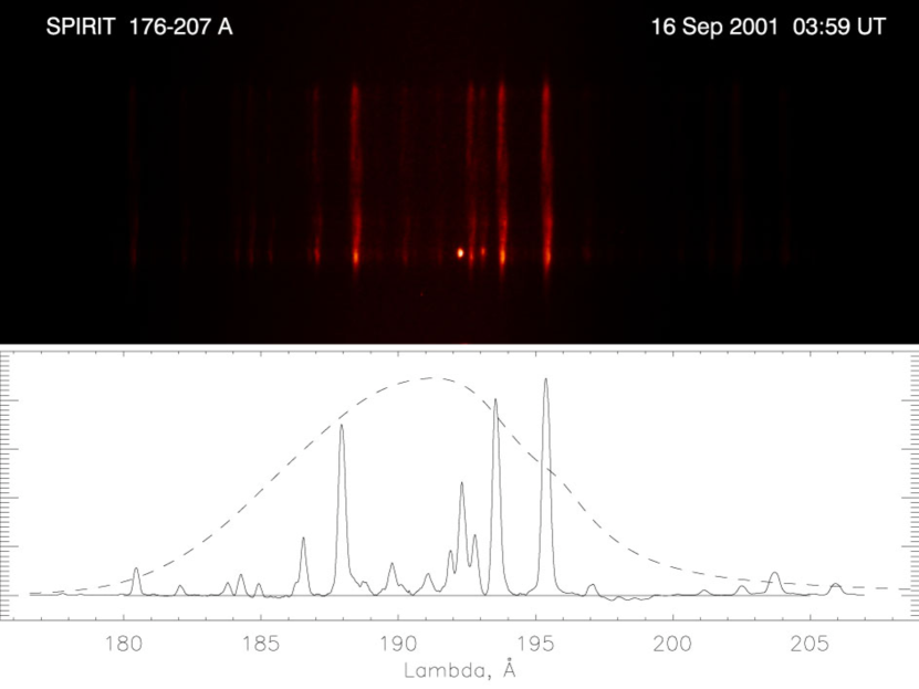
Figure 6: Top panel: the V190 spectoheliogram registered on 2001 Sep 9, convolved with EIT 195 Å bandpass function. Bottom panel: solid line — SPIRIT spectra from the forementioned spectroheliogram integrated along the spatial axis and multiplied by EIT 195 Å bandpass function. Dashed line — normalized EIT 195 Å bandpass function.

4 Results

We have analysed spectra of the four flares and note three main results of our analysis:

• A catalog of EUV spectral lines observed in large solar flares;

• DEM and $n_{e}$ of the emitting plasma;

• A benchmark of the atomic database, by analysing ratios of the observed and calculated spectral line intensities.

4.1 Catalog of spectral lines

Comparisons of observational and fitted spectra are given in Figure 7 (V190) and Figure 8 (U304). The black curve denotes observational data, blue vertical lines denote individual spectral lines from the catalog, and the red curve denotes fitted spectra.

The catalog of spectral lines is given in Table 4.1 (V190 channel) and Table 4.1 (U304 channel). Only the strongest 70 lines were included in the tables, but during the identification we operated with a larger number of lines.

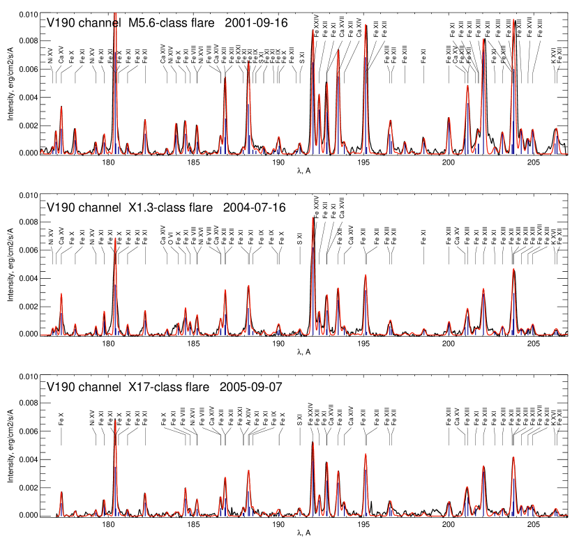
Figure 7: V190 spectra of flares: X1.3 observed on 2004-07-16; M5.6 observed on 2001-09-16; and X17 observed on 2005-09-07. The black curve denotes observational data, blue vertical lines denote individual spectral lines from catalog, and the red curve denotes fitted spectra (calculated using instrument FWHM).

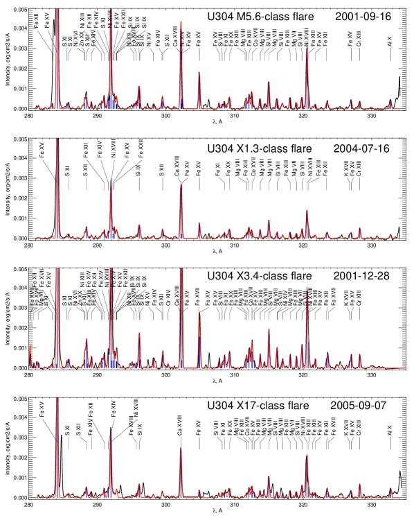
Figure 8: U304 spectra of flares: X1.3 observed on 2004-07-16; M5.6 observed on 2001-09-16; X17 observed on 2005-09-07; and X3.4 observed on 2001-12-28. The black curve denotes observational data, blue vertical lines denote individual spectral lines from catalog, and the red curve denotes fitted spectra (calculated using instrument FWHM).

Table 3: Intensities of spectral lines [$\cdot 10^{-5}$ erg/s/cm²] in the solar flares in the V190 channel.

Note. — Columns correspond to different flares, rows denote different spectral lines. The flux in a particular spectral line corresponds to the whole flaring region (and do not contain $\frac{1}{sr}$ factor). Minus ’–’ sign denotes that the line was too weak in a particular spectrum, ’N/A’ in the X3.4 flare means that the flare was not observed by V190 channel of SPIRIT.

Table 4: Intensities of spectral lines [$\cdot 10^{-5}$ erg/s/cm²] in the U304 channel.

Note. — Columns correspond to different flares, rows denote different spectral lines. The flux in a particular spectral line corresponds to the whole flaring region (and do not contain $\frac{1}{sr}$ factor). Minus ’–’ sign denotes that the line was too weak in a particular spectrum.

In the V190 channel the strongest lines are: Fe X 177.25 Å, Fe XI 180.41 Å, selfblend Fe XII 186.85+.89 Å, selfblend Fe XI 188.23+.29 Å, Fe XXIV 192.03 Å, Fe XII 192.39 Å, blend of Fe XI 192.83 + Ca XVII 192.85 Å, Fe XII 193.51 Å, Fe XII 195.12 Å, Fe XIII 196.54 Å, Fe XII 196.63 Å, Fe XIII 200.02 Å, Fe XIII 202.04 Å, selfblend Fe XIII 203.80+.83 Å, which have intensities of order $2\cdot 10^{-4}\mbox{ erg/s/cm${}^{2}$}$ and higher.

In the U304 channel the strongest lines are: Fe XV 284.16 Å, blend S XII 288.42 Å+ Fe XIV 289.15 Å, Ni XVIII 291.98 Å, selfblend Si IX 296.11+.21 Å, Ca XVIII 302.19 Å, blend Fe XVII 304.82 Å+ Fe XV 304.89 Å, Mg VIII 315.02 Å, blend Ni XVIII 320.57 Å+ Fe XIII 320.81 Å, which have intensities of order $2\cdot 10^{-4}\mbox{ erg/s/cm${}^{2}$}$ and higher. The strongest line in the spectral region — the Si XI/He II blend with $\lambda\sim 304$ Å was removed from the spectra before the analysis.

Emission of hot spectral lines such as Fe XXIV 192.03 Å ($T_{m}=16$ MK), Ca XVII 192.85 Å ($T_{m}=6.3$ MK), Fe XXII 292.46 Å ($T_{m}=13$ MK), Ca XVIII 302.19 Å ($T_{m}=10$ MK), Fe XX 309.29 Å ($T_{m}=10$ MK) is produced only during flares. Spectral images of a flare in these lines are compact and usually not intermingled with other spectral lines (we inspected a large number of the SPIRIT spectroheliograms). Thus, these lines can be used for detection of a solar flare and they are ideal for high-temperature DEM and Doppler shift analysis.

The obtained spectra of all flares are similar, but still there are some differences. Absolute fluxes in separate spectral lines measured by SPIRIT in the M5.6 and X3.4 are similar and twofold higher than those in the X1.3 and X17 flares. The decrease is in direct correlation with the decrease of the total flux in the EIT images. The decrease may be caused by variation in solar irradience — the M5.6 and X3.4 flares were registered at the end of 2001 (near the maximum of solar activity), the X1.3 was observed on July 2004, and the X17 flare was observed on September 2005 (near the minimum of solar activity), as well as degradation of EIT sensitivity (BenMoussa et al., 2013).

4.2 Plasma diagnostics

The result of the DEM reconstruction is presented in Figure 9: red lines correspond to different runs (we used 100 runs), black line is an average (median) DEM, and a green line denotes initial DEM, obtained on the 0-level step.

The obtained DEMs have a similar shape — a local minimum at $T\sim 0.6-0.8$ MK (cold plasma), a local maximum at $T\sim 2.5$ MK (warm plasma), and a global maximum at $T\sim 10$ MK (hot plasma). The two-peaks shape may be associated with different structures: the warm plasma fill loops, which are adjacent to the flaring region (Schmelz et al., 2011), whereas the hot plasma is produced in the flaring region. The M5.6 and X1.3 flares have narrower hot-component peaks, which may be attributed to the earlier phases of the flare decays ($\Delta\tau\sim 10$ and $7$ minutes after the flare maxima). The X3.4 and X17 were registered on later phases ($\Delta\tau\sim 40$ and $\sim 3$ hours after the flare maxima), therefore the hot plasma had time to warm up the surroundings. The warm-component peak in the latter two flares has two-peaks shape with $T_{1}=1.6$ MK (both flares) and $T_{2}=2.5$ MK (the X3.4 flare) and $T_{2}=4.0$ MK (the X17 flare). These double peaks in warm plasma may also be attributed to spatially separated structures.

The steep decrease in DEMs with $T>10$ MK observed in the M5.6, X1.3 and X17 flares is determined by the intensities of hot lines, among which are Ca XVII ($T_{m}=6.3$ MK), Fe XXII ($T_{m}=13$ MK), Ca XVIII ($T_{m}=10$ MK), Fe XX ($T_{m}=10$ MK), but the primary contribution is definitely due to the Fe XXIV 192.03 Å line, which has $T_{m}=16$ MK. Since the V190 channel observations were unavailable for the X3.4 flare, it is possible that DEM values with $T>10$ MK are overestimated in the flare.

The confidence level of the DEMs is assessed by the relative spread of different DEM solutions and amounts as much as a factor of 2 (each solution from the range equally well describes the observational data, so each solution from the range is equally possible).

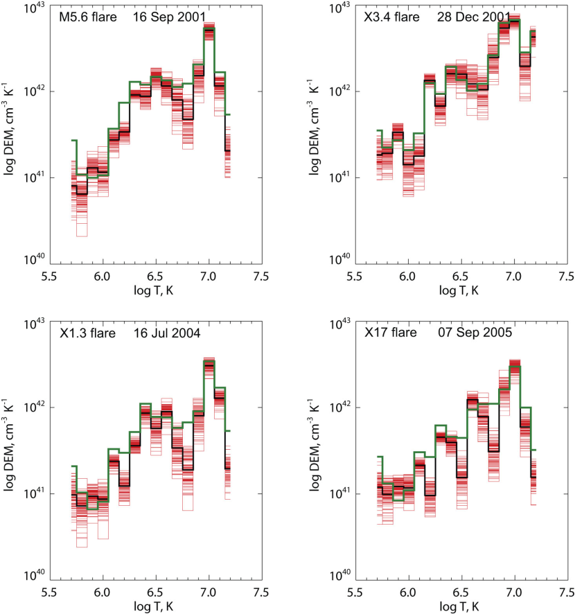
Figure 9: DEMs of the flares. Red lines denote DEMs obtained during different iterations of the GA procedure, black lines denote average value, and a dashed line denotes DEM, obtained during 0-level analysis.

The results of $n_{e}$ analysis are presented on Figure 10 — the L-functions of the Fe XI, Fe XII, Fe XIII and Fe XV ions for the M5.6, X1.3 and X17 flares are given (black lines denote V190, red lines denote U304). Whereas L-functions of a single ion should cross in a single point, one can see considerable disagreement in several cases. We note that during the iterative steps we tried to improve the agreement of the L-functions varying the intensities of blended lines; however, better agreement was not reached.

The best consistency among different spectral lines is observed in the Fe XII ion. The $n_{e}$ values are $\sim 6.5\times 10^{9}$ cm^-3 (the L-functions intersect in the range $\log n_{e}=[9.7-9.9]$) in all flares. The most reliable Fe XI lines — 179.76, 180.41, 188.23 Å — also favour this value. The L-functions of the Fe XIII ion show considerable discrepancy. The 200.02, 202.04, and the blend $203.80+.83$ Å lines show systematically lower density $n_{e}\sim 2\times 10^{9}$ cm^-3, whereas 196.54 and 200.02, $203.80+.83$ Å lines cross at density $\sim 6.5\times 10^{9}$ cm^-3. The Fe XV lines show systematic discrepancies in all flares. We will discuss possible causes of the discrepancies in the next section. We used a value of $n_{e}=6.5\times 10^{9}$ cm^-3 for all the flares for DEM analysis and calculation of synthetic spectra.

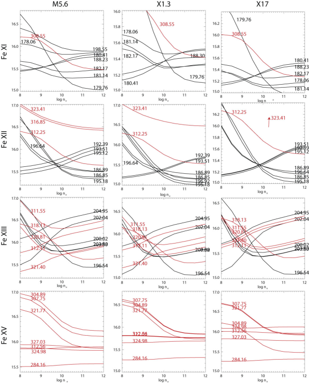
Figure 10: The L-function of Fe XI–Fe XIII, and Fe XV ions for the M5.6, X1.3 and X17 flares. Black lines denote spectral lines from the V190 channel; red lines denote the U304 channel.

4.3 Comparison of observational and theoretical line intensities

We compared the observational and theoretical intensities using different approaches: in the DEM reconstruction procedure, by using L-function plots, and by comparing observational and synthetic spectra. All these approaches, in essence, consist of comparison of observational and theoretical line intensities, whereas each approach gives some additional convenience in data analysis.

In the vast majority of spectral lines the correspondence of observational and theoretical intensity is within factor of 2. The most striking discrepancy $R$ (ratio of observational/theoretical intensity) is observed in the DEM reconstruction in the following lines: Fe XII 323.41 Å ($\sim 8$), Fe XIII 312.11 Å ($\sim 2.5$), Fe XII 312.25 Å ($\sim 2.5$), Fe XIII 202.04 Å ($\sim 2.0$), Fe XVII 323.65 Å ($\sim 0.7$), Fe XV 327.05 Å ($\sim 0.7$). There is also a systematic discrepancy in relative intensities of Mg VIII and Si VIII lines — whereas these spectral lines have similar dependence on temperature and density, the ratio $R$ for Mg VIII is constantly higher and for Si VIII is constantly lower than 1. The L-function plots show discrepancies in the Fe XIII and Fe XV lines. Comparison of the observational and synthetic spectra reveal several discrepancies in other lines. The observed discrepancies are typical for the analyzed flares, and we will discuss them all together.

The observed intensity of the Fe XII 323.41 Å line is approximately 8 times higher than those, predicted in the DEM reconstruction. The discrepancy can not be attributed to problems with SPIRIT spectral sensitivity due to good correspondence of other intense lines with close wavelengths. The Fe XII 323.41 Å line is blended with Fe XVII 323.65 Å; however, the spectral profile of the blend seems unlikely to the blend of two close spectral lines. The incorrect identification of one of the lines seems quite reasonable.

The next two lines with ratio $R\sim 2.5$ are Fe XIII 312.11 Å and Fe XII 312.25 Å. The lines fall within a wide blend, which encompassess Fe XIII 311.55 Å, Ni XV 311.76 Å, Mg VIII 311.76 Å, Fe XIII and Fe XII, Co XVII 312.54 Å, Fe XV 312.56 Å, and Fe XIII 312.87 Å (the strongest lines according to the synthetic spectra). Detailed analysis of the blend deserves effort and attention; a quick look (using both spectra in Figure 8 and L-functions in Figure 10) shows no simple solution for improving the $R$ ratios neither via changes of $n_{e}$, nor changes of relative intensity of lines involved in the blend. Fortunately, in the U304 channel there are a number of strong lines suitable for reconstruction of intensities of Mg VIII and Fe XIII spectral lines.

The Fe XIII 202.04 Å line is among the most intense lines of the Fe XIII ion; however, its ratio $R$ is approximately 2 in all analyzed flares. The observed discrepancy cannot be attributed to problems with SPIRIT spectral sensitivity, since the line falls between other strong Fe XIII lines — 200.02 Å and a blend of $203.80+.83$ Å (observed intensity of these lines is consistent with theory). During the DEM reconstruction other Fe XIII lines (196.54, 200.02, 203.80, 312.11, 318.13, and 320.81 Å) were predicted with higher accuracy (usually better than 40%), eliminating possible issues with abundances or temperature distribution of the emitting plasma. The L-functions of all Fe XIII lines are density-sensitive (see Figure 10) and correction of the $n_{e}$ value seems reasonable and sufficient. However, the L-functions of the 200.02, 203.80, 203.83, and 320.81 Å lines have the same dependence on density and their absolute values are in a good agreement with theory. Density values $n_{e}$ obtained by the crossing of the 202.04 Å line and 200.02 and $203.80+.83$ Å lines, is systematically lower ($\sim 2\times 10^{9}$ cm^-3) than $n_{e}$ obtained with the Fe XI and Fe XII ions, which favors against the 202.04 Å line. A good agreement with the density $n_{e}$, obtained with the Fe XI and Fe XII ions, was obtained by crossing the L-functions of the 196.54 Å line with the 200.02, $203.80+.83$ Å lines. This result is in a slight contradiction with Brosius et al. (1998) and Shestov et al. (2009), who found good correspondence of the $n_{e}$ values measured by Fe XI and Fe XIII lines. The L-functions of the 204.95, 312.11, and 321.40 Å lines have similar behavior with density, and in some flares their absolute values are in a good agreement. However, the L-function of the 204.95 Å line does not produce a reasonable $n_{e}$ value (observed $n_{e}<10^{9}$ cm^-3). In two flares (M5.6 and X1.3) the L-function of the 321.40 Å line has a common crossing with the 196.54, 200.02, and $203.80+.83$ Å lines, which confirms the correctness of the latter lines.

Given the above information, overall agreement of the Fe XIII L-functions may be improved by decreasing the L-functions of the 202.04 Å line by factor of $\sim 2$ and of the 204.95 Å line by factor of $\sim 4$. The observed excess in the L-functions may be caused by unaccounted blending of spectral lines or inappropriate atomic data. The atomic structure of the Fe XIII ion has recently been extensively studied by Del Zanna (2011), and the author did not find any problems with the ion. However, observed discrepancies in the SPIRIT data (with no strong blend candidates provided by CHIANTI) and inconsistency in the $n_{e}$ values obtained with Fe XIII indicate that some questions still remain.

The Fe XVII 323.65 Å line has a ratio $R\sim 0.7$ and is blended with Fe XII 323.41 Å. The latter line shows a striking discrepancy with $R\sim 8$). The spectral profile of the blend seems unlikely to the blend of two close spectral lines, and wrong identification of one of the lines seems quite reasonable.

The Fe XV 327.03 Å line has a ratio $R\sim 0.7$. It is blended with K XVII 326.78 Å  and taking into account that both lines are on the edge of the SPIRIT spectral range, the ratio $R$ is not too bad.

The other issue is the systematic discrepancy of intensities between the Mg VIII and Si VIII spectral lines. The two ions have similar atomic structure ($2s2p^{2}\rightarrow 2s^{2}2p$ transitions in Mg VIII and $2s2p^{4}\rightarrow 2s^{2}2p^{3}$ transitions in Si VIII), similar abundances (both in coronal and photospheric models), close wavelengths — 311.77, 313.74, 315.02, and 317.03 Å (Mg VIII) and 314.36, 316.22, 319.84 Å (Si VIII) — and contribution functions of the lines have similar dependence on temperature and density. Nevertheless, ratios $R$ for Mg VIII lines are 1.6, 1.4, and 1.03 for the 313.74, 315.02, and 317.03 Å lines (averaged by flares), whereas the ratios $R$ for Si VIII approach 0.7, 0.6, and 0.8 for the 314.36, 316.22, 319.84 Å lines. Inadequate abundances are the most likely cause of the discrepancy. A similar possibility was pointed out by Schmelz et al. (2012) in their analysis of SERTS data.

The L-functions of the Fe XV ion can be separated into two groups: those that decrease with density (the 304.89, 307.75, and 321.77 Å lines) and those that do not change with density (the 284.16, 312.56, 324.98, and 327.03 Å lines). The L-functions inside each group should coincide. According to the observational data, the L-function of the 284.16 Å line is usually 4 times lower than the others. The discrepancy can be caused by different factors: the SPIRIT detector saturation, problems with SPIRIT spectral sensitivity, optical thickness of the emitting plasma, and others. That is why the 284.16 Å line was not taken into account in the DEM reconstruction. The two L-function groups are likely to cross at densities $n_{e}>10^{10}$ cm^-3 (higher than the density obtained by the Fe XI and Fe XII ions).

The other method for analyzing the correspondence of observational data with theoretical values is comparison with unmodified synthetic spectra — that was calculated using DEM and $n_{e}$ (and other model parameters) and has not been modified to match observational data. Such a comparison for the M5.6 flare is given in Figure 11. The main discrepancies are observed in the V190 channel, with the $R$ ratios of different lines being both larger and smaller than the unity: Ni XV 176.74 Å ($R\ll 1$), Ca XV 176.93 Å ($R\gg 1$), Fe X 177.24 Å ($R\sim 0.5$), Fe XI 178.06 Å ($R\sim 2$), line with $\lambda\sim 186.00$ Å (candidates are Ni XV 185.73 Å, Fe XIII 185.76 Å and Fe XII 186.24 Å, which all have $R\ll 1$). Many spectral lines of the Fe XIII ion with wavelengths $\lambda\sim 200-205$ deviate from theoretical values. In the U304 channel the spectral lines are more or less consistent with the theory, with the following exceptions: Fe XV 284.16 Å ($R\sim 0.25$), Fe XV 292.28 Å ($R\sim 0.5$), blend of Fe XVII 304.82 + Fe XV 304.89 Å ($R\sim 0.5$), Si VIII 308.19 Å ($R\sim 3$), complex blend with $\lambda\sim 312$ Å (Mg VIII, Fe XIII, Fe XII, Co XVII and others ions), Mg VIII 315.02 Å, Fe XII 323.41 Å.

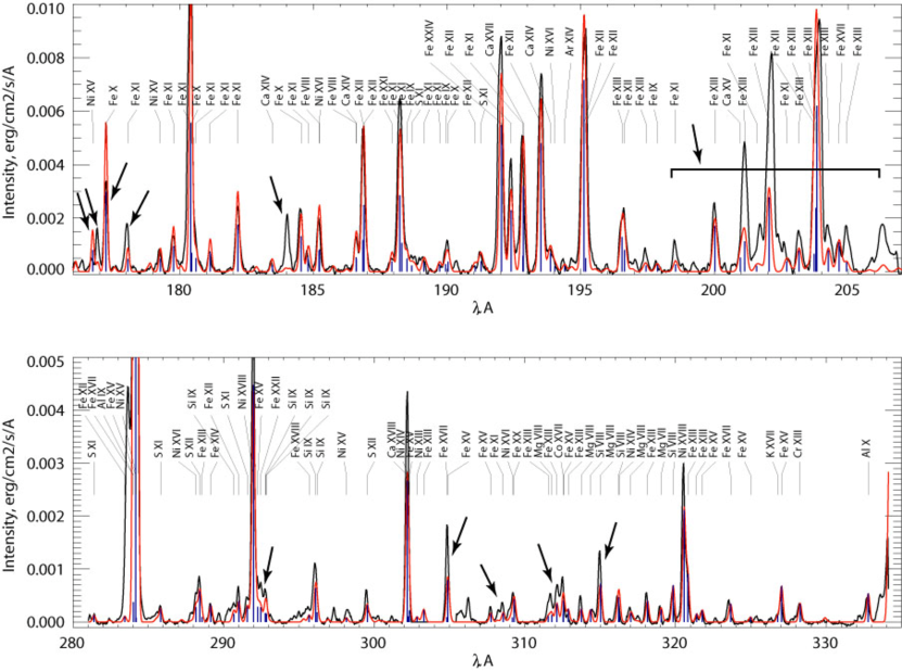
Figure 11: Comparison of observational and synthetic (calculated using DEM and $n_{e}$ with CHIANTI) spectra for the M5.6 flare. Top panel — V190 channel, bottom panel — U304 channel. The black curve denotes observational data, blue vertical lines denote individual spectral lines, and the red curve denotes synthetic spectra (calculated using instrument FWHM). The arrows show major discrepancies of observational and synthetic spectra.

5 Discussion

During the identification we fit observational data with synthetic spectra calculated using CHIANTI. The procedure does not take into account unknown lines, and this is the main disadvantage of the proposed method of the identification. However, comparison of observed and calculated intensities gives a lot of information about the reliability (qualitative — correct or incorrect) and accuracy (quantitative — say 10% or 50%) of the identification. The accuracy depends on two factors — a) quality of the observational data (accuracy of spectral calibration, low noise, absence of scattered light in the instrument, the compactness of the emitting plasma etc.); b) accuracy of the used atomic data.

We analyzed how the identification of the obtained spectra depended on the relative calibration of SPIRIT and conclude that the relative calibration is better than a factor of 2 (there are a number of lines whose intensity ratio do not depend on density and which comply with theory). The absolute calibration was obtained using simultaneous EIT images — 195 Å for the V190 channel and 304 Å for the U304 channel. After the absolute calibration, the average line intensities in the both channels (which were calibrated independently) satisfy each other. However, the resulting absolute calibration of SPIRIT is as good as EIT calibration. Any errors in EIT calibration — for example due to the decay of the EIT sensitivity (BenMoussa et al., 2013) — will affect the absolute calibration of the presented spectra.

We analyzed how the results of the DEM reconstruction depend on the errors (up to 30%), artificially introduced into the observational data. The obtained discrepancy turned out to be within the DEM confidence level, obtained in the genetic algorithm. Other factors (beside adequate identification) do not play such an important role in the final accuracy. We assess the final accuracy of the observational data (including the absolute calibration) to be a factor of 4.

The performed analysis of simultaneous EIT and SPIRT data proved that telescopic and spectroscopic observations significantly enhance each other. SPIRIT gives direct information about the relative flux in each spectral line contributing to the EIT image, and relative flux measured by EIT (in dn units) allows to calibration of uncalibrated SPIRIT data. Using spectroscopic instrumentation with relatively high spectral resolution could enhance the informational content of other instruments, like AIA or EVE.

The other important aspect for spectroscopic analysis is spectral resolution. The instrumental resolution of SPIRIT is $\sigma\sim 0.1$ Å (for comparison, the spectral resolution of EIS is $\sigma\sim 0.020$ Å). Many strong and important lines are not resolved by SPIRIT, such as the Fe XIII 203.80 and 203.83 Å lines, or Ni XVIII 291.98 Å, Fe XV 292.26 Å, and Fe XXII 292.45 Å lines. Nevertheless, the identification procedure used, allowed the deconvolution of blends and the calculation of intensities. In some cases we obtained good correspondence of observational and theoretical intensities: the example is the blend of the Fe XIII 203.80 and 203.83 Å lines, which are in a good agreement with the Fe XIII 200.02 Å line; the blend of the Fe XIII 196.54 Å and Fe XII 196.64 Å lines also complies with the rest of the Fe XII and Fe XIII. In some cases agreement was not achieved: the multiple blend with $\lambda\sim 312$ Å is an example, where the lines contributing to the blend show poor correspondence with the theory. Nevertheless, the method of deconvolving blends using a synthetic spectrum is a powerful tool for spectroscopic analysis.

Let’s compare the calculated DEMs with those obtained from other instruments. The DEM which is widely used for modelling of the EUV spectra is that presented by Dere & Cook (1979) (this DEM is actually provided by CHIANTI as a flare.dem). The authors analyzed the decay phase of an M2 flare using observations from the S082A EUV spectroheliograph and the S082B UV spectrograph aboard Skylab. During the DEM calculation the authors used the quantity “total line power radiated by the plasma” (which actually coincides with our approach). However, the DEM values provided by CHIANTI are expressed in units cm^-5 K^-1. The DEMs, calculated in our analysis correspond to the whole flaring region, and we need to assess the area associated with the flare. In order to assess the area we inspected monochromatic images of the flares and conclude that the images have symmetrical Gaussian shape with typical FWHM $\sim 8$ pixels (good examples are the bright lines of the Ni XVIII, S XII, Ca XVIII ions in Figure 3). This is the minimal size of the structure observed on the spectroheliograms, and the size is determined by the PSF of the instrument (primarily, its focusing mirror). Thus, the spatial size of a flare should not exceed $\sim 3\times 3$ pixels so as not to increase flare images. Taking into account the angular size of a pixel of SPIRIT — 6.7 arcsec, we obtain that $3\times 3$ pixels correspond to the area $2\cdot 10^{18}$ cm². We multiply flare.dem from CHIANTI by this factor and compare it with the current DEMs. The correspondence is good enough: beside similar shape (local minima and maxima coincide in the two datasets) we get compliance of the orders of magnitude — $\sim 8\times 10^{40}$ cm^-3 K^-1 (cold component) and $\sim 6\times 10^{42}$ cm^-3 K^-1 (hot component).

We performed another verification of the calculated DEMs: we simulated GOES X-ray fluxes using the calculated DEMs and GOES response functions (goes_resp2.dat from Solar Software). The calculated fluxes complied within an order of magnitude or better with those, actually measured by GOES.

To investigate heating dynamics in observed flares — impulsive or continuous — we compared hot component lifetime ($\tau_{life}$, few hours) with its conductive cooling time ($\tau_{cond}$): if $\tau_{cond}\ll\tau_{life}$, then heating is continuous; if $\tau_{cond}\sim\tau_{life}$, then heating is impulsive. We estimated $\tau_{cond}$ with the formula (Culhane et al., 1994):

$$\tau_{cond}=\frac{21n_{e}k_{b}h^{2}}{5\kappa T^{5/2}}$$ (4)

where, $n_{e}$ — plasma electron density, $k_{b}$ — Boltzmann constant, $h=1.5\times 10^{7}$ m — characteristic size, $\kappa=9.2\times 10^{-7}$ erg s^-1 cm^-1 K^-7/2 — the Spitzer conductivity, $T=10$ MK — plasma temperature. Electron density in flares ranges from $10^{10}$ cm^-3to $10^{12}$ cm^-3  (Milligan et al., 2012). For $n_{e}=10^{10}$ cm^-3 $\tau_{cond}\sim$ 30 seconds ($\tau_{cond}\ll\tau_{life}$), which requires continuous heating; for $n_{e}=10^{12}$ cm^-3 $\tau_{cond}\sim$ 1 hour ($\tau_{cond}\sim\tau_{life}$), which favors impulsive heating. SPIRIT spectra don’t have high-temperature spectral lines, suitable for the density diagnostics, so we estimate $n_{e}$ using the obtained DEMs:

$$EM_{hot}\sim n_{e}^{2}h^{3}\Rightarrow n_{e}\sim\sqrt{\frac{EM_{hot}}{h^{3}}}\sim 10^{11}\ \textmd{cm${}^{-3}$}$$ (5)

This is a rough estimation: the DEMs accuracy is a factor of 4, and the real volume of the hot component is probably less than $h^{3}$ (most likely it is not spherical, but has loop-like geometry). So $n_{e}$ is probably closer to $10^{12}$ cm^-3 than to $10^{10}$ cm^-3, and heating in observed flares is most likely impulsive.

6 Conclusion

Initially, the main goal of the work was to present unique observational data — EUV spectra of large solar flares, observed by the SPIRIT spectroheliograph. Due to the relatively low spectral resolution of SPIRIT, many lines are blended, which prevents a straightforward method for line identification and measurement. The original procedure for spectra analysis, based on calculation of synthetic spectra and measurement of plasma DEM and $n_{e}$, not only allowed identification and measurement of intensity of as many as 70 spectral lines in each spectral band in each flare, but also provided a lot of other important information. The performed spectroscopic analysis demonstrated the accuracy of the adopted spectral calibration of the SPIRIT spectroheliograph. Simultaneous observations of the EIT telescope and the SPIRIT spectroheliograph allowed calculation of absolute fluxes in each spectral line.

Whereas the analysed flares belong to different X-ray classes and were registered on different stages of their decay, registered spectra and calculated DEMs have many in common. All DEMs have similar shape with global maxima at $T\sim 10$ MK and local maxima at $T\sim 2.5$ MK.

The performed comprehensive analysis allowed interpretation of observational data with good quality — most of the spectral line intensities correspond to their theoretical values with 40% accuracy. The remaining lines with consistency of a factor of 2 and worse require additional analysis, which may involve, along with refinement of spectral calibration, more complicated plasma models, verification of abundances or atomic rates etc.

The registered spectra, as well as proposed identification and DEMs, could be used for further spectral analysis. The obtained spectra, synthetic spectra, DEMs, and proposed IDL software are available at http://xras.lebedev.ru/SPIRIT/ or on request from S. Shestov.

References

- BenMoussa et al. (2013) BenMoussa, A., Gissot, S., Schühle, U., et al. 2013, Sol. Phys.
- Brosius et al. (1998) Brosius, J. W., Davila, J. M., & Thomas, R. J. 1998, The Astrophysical Journal Supplement Series, 119, 255
- Brosius et al. (1996) Brosius, J. W., Davila, J. M., Thomas, R. J., & Monsignori-Fossi, B. C. 1996, The Astrophysical Journal Supplement Series, 106, 143
- Chamberlin et al. (2012) Chamberlin, P. C., Milligan, R. O., & Woods, T. N. 2012, Sol. Phys., 279, 23
- Culhane et al. (1994) Culhane, J. L., Phillips, A. T., Inda-Koide, M., et al. 1994, Sol. Phys., 153, 307
- Culhane et al. (2007) Culhane, J. L., Harra, L. K., James, A. M., et al. 2007, Sol. Phys., 243, 19
- Czaykowska et al. (1999) Czaykowska, A., de Pontieu, B., Alexander, D., & Rank, G. 1999, in ESA Special Publication, Vol. 448, Magnetic Fields and Solar Processes, ed. A. Wilson & et al., 773
- Del Zanna (2011) Del Zanna, G. 2011, A&A, 533, A12
- Del Zanna et al. (2011) Del Zanna, G., Mitra-Kraev, U., Bradshaw, S. J., Mason, H. E., & Asai, A. 2011, A&A, 526, A1
- Del Zanna et al. (2006) Del Zanna, G., Schmieder, B., Mason, H., Berlicki, A., & Bradshaw, S. 2006, Sol. Phys., 239, 173
- Dere (1978) Dere, K. P. 1978, The Astrophysical Journal, 221, 1062
- Dere & Cook (1979) Dere, K. P., & Cook, J. W. 1979, ApJ, 229, 772
- Dere et al. (1997) Dere, K. P., Landi, E., Mason, H. E., Monsignori Fossi, B. C., & Young, P. R. 1997, Astronomy and Astrophysics Supplement Series, 125, 149
- Dere et al. (2009) Dere, K. P., Landi, E., Young, P. R., et al. 2009, A&A, 498, 915
- Doschek et al. (2013) Doschek, G. A., Warren, H. P., & Young, P. R. 2013, ApJ, 767, 55
- Harrison et al. (1995) Harrison, R. A., Sawyer, E. C., Carter, M. K., et al. 1995, Sol. Phys., 162, 233
- Hudson et al. (2011) Hudson, H. S., Woods, T. N., Chamberlin, P. C., et al. 2011, Sol. Phys., 273, 69
- Landi & Landini (1998) Landi, E., & Landini, M. 1998, Astronomy and Astrophysics, 340, 265
- Malinovsky & Heroux (1973) Malinovsky, M., & Heroux, L. 1973, The Astrophysical Journal, 181, 1009
- Milligan et al. (2012) Milligan, R. O., Kennedy, M. B., Mathioudakis, M., & Keenan, F. P. 2012, ApJ, 755, L16
- Neupert et al. (1992) Neupert, W. M., Epstein, G. L., Thomas, R. J., & Thompson, W. T. 1992, Solar Physics, 137, 87
- O’Dwyer et al. (2011) O’Dwyer, B., Del Zanna, G., Mason, H. E., et al. 2011, A&A, 525, A137
- Oraevsky & Sobelman (2002) Oraevsky, V. N., & Sobelman, I. I. 2002, Astronomy Letters, 28, 568
- Parenti et al. (2003) Parenti, S., Landi, E., & Bromage, B. J. I. 2003, ApJ, 590, 519
- Schmelz et al. (2012) Schmelz, J. T., Kimble, J. A., & Saba, J. L. R. 2012, ApJ, 757, 17
- Schmelz et al. (2011) Schmelz, J. T., Rightmire, L. A., Saar, S. H., et al. 2011, ApJ, 738, 146
- Shestov et al. (2010) Shestov, S. V., Kuzin, S. V., Urnov, A. M., Ul’Yanov, A. S., & Bogachev, S. A. 2010, Astronomy Letters, 36, 44
- Shestov et al. (2009) Shestov, S. V., Urnov, A. M., Kuzin, S. V., Zhitnik, I. A., & Bogachev, S. A. 2009, Astronomy Letters, 35, 45
- Siarkowski et al. (2008) Siarkowski, M., Falewicz, R., Kepa, A., & Rudawy, P. 2008, Annales Geophysicae, 26, 2999
- Thomas & Neupert (1994) Thomas, R. J., & Neupert, W. M. 1994, The Astrophysical Journal Supplement Series, 91, 461
- Tousey et al. (1977) Tousey, R., Bartoe, J.-D. F., Brueckner, G. E., & Purcell, J. D. 1977, Aplied Optics, 16, 870
- Tripathi et al. (2011) Tripathi, D., Klimchuk, J. A., & Mason, H. E. 2011, ApJ, 740, 111
- Tripathi et al. (2010) Tripathi, D., Mason, H. E., Del Zanna, G., & Young, P. R. 2010, A&A, 518, A42
- Ugarte-Urra et al. (2005) Ugarte-Urra, I., Doyle, J. G., & Del Zanna, G. 2005, A&A, 435, 1169
- Watanabe et al. (2010) Watanabe, T., Hara, H., Sterling, A. C., & Harra, L. K. 2010, ApJ, 719, 213
- Woods et al. (2012) Woods, T. N., Eparvier, F. G., Hock, R., et al. 2012, Sol. Phys., 275, 115
- Zhitnik et al. (2002) Zhitnik, I. A., Bougaenko, O. I., Delaboudiniere, J.-P., et al. 2002, in ESA Special Publication, Vol. 506, Solar Variability: From Core to Outer Frontiers, ed. J. Kuijpers, 915–918