Fluctuation Amplitude of a Trapped Rigid Sphere
Immersed in a Near-Critical Binary Fluid Mixture
within the Regime of the Gaussian Model

Abstract

The position of a colloidal particle trapped in an external field thermally fluctuates at equilibrium. As is well known, the ambient fluid is not a simple heat bath and the particle mass appears to increase, which influences the mean square velocity of the particle. In this study, we suppose that the particle is surrounded by a binary fluid mixture in the homogeneous phase near, but not too close to, the critical point. Usually, one component is preferably attracted by the particle surface, and the resultant adsorption layer becomes significant because of the near-criticality. When the particle fluctuates in this situation, its mean square displacement should also be influenced by the ambient fluid because the adsorption layer does not follow the particle motion totally. We calculate the influence in a simple case, where a rigid spherical particle fluctuates with a small amplitude and its surface attracts one component weakly. We utilize the hydrodynamics in the limit of no dissipation to examine the contribution from the ambient mixture to the equal-time correlation, which is shown to be reduced by an additional stress, including osmotic pressure.

I Introduction

Suppose a colloidal particle, about $0.1$–$1\ \mu$m in size, trapped by optical tweezers. The particle position fluctuates at equilibrium, which is experimentally observed with high resolutions of space ($<1$ nm) and time ($<1\ \mu$s) lukic ; nat ; natp ; grim . For simplicity, we assume the one-dimensional motion of a rigid sphere (mass $m$) trapped in a harmonic potential (natural angular frequency $\omega_{0}$) to consider the fluctuation. The positional deviation of the particle center from the potential bottom is denoted by $\zeta$, while the equilibrium average at the temperature $T$ is indicated by $\langle\cdots\rangle$. The equal-time correlations can be calculated as

$$\langle\zeta^{2}\rangle={k_{\rm B}T\over m\omega_{0}^{2}}\quad{\rm and}\quad\langle\left({d\zeta\over dt}\right)^{2}\rangle={k_{\rm B}T\over m+m_{\rm ind}}\ .$$ (1)

Here, $k_{\rm B}$ denotes the Boltzmann constant, while $m_{\rm ind}$ denotes the induced mass, which equals half the mass of the displaced fluid lamb . The ambient fluid cannot be regarded as a heat bath; the particle mass appears to increase because the particle motion causes flow. The induced mass can be calculated in terms of the hydrodynamics for a one-component fluid.

In Eq. (1), the mean square displacement $\langle\zeta^{2}\rangle$ is not influenced by the fluid motion. It is expected not to be the case, however, if the ambient fluid is a near-critical binary fluid mixture. The reason is as follows. It is usual that one component is preferably attracted by the particle surface Cahn . Suppose that the correlation length of the mixture is several nanometers, which is much smaller than the particle radius, and that the ambient fluid is in the homogeneous phase. The adsorption layer, where the preferred component is more concentrated, appears around the particle and has a thickness comparable to the correlation length binder ; holyst . The adsorption layer is isotropic when the particle is fixed, as is drawn schematically in Fig. 1(a). There, although the resultant gradient of the mass-density difference between the two components generates osmotic pressure, the total force exerted on the particle by the ambient fluid vanishes. When the particle moves rather rapidly, the adsorption layer cannot follow the motion and is deformed, as shown in Fig. 1(b). Then, the additional force due to the gradient of the mass-density difference can be exerted on the particle in total. It is thus possible that the ambient fluid influences the mean square displacement, unlike in Eq. (1). In this paper, we calculate this influence in a simple case. We assume the particle to be neutral electrically and no ion to be involved in the mixture.

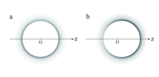
Figure 1: Cross section of a spherical particle immersed in a near-critical binary fluid mixture is schematically drawn. The gray scale reflects the mass-density difference between the two components; the shaded region represents the adsorption layer. (a) The particle is fixed with its center being located at the origin $O$. The adsorption layer is concentric with the particle contour in this figure; the mass-density difference is isotropic as viewed from the particle center. (b) At a transient position of the particle in its motion along the $z$-axis, the adsorption layer is deformed to become anisotropic because the ambient fluid is not shifted translationally.

We refer to some backgrounds. In this paragraph, we mention how the induced mass appears in Eq. (1), where the ambient near-criticality combined with the preferential attraction is not assumed. The evolution of the particle position $\zeta$ with respect to the time $t$ can be described by the Langevin equation kubo ; grim

$$m{d^{2}\over dt^{2}}\zeta(t)=-m\omega_{0}^{2}\zeta(t)+F_{\rm hy}(t)+F_{\rm th}(t)\ ,$$ (2)

where $F_{\rm hy}$ and $F_{\rm th}$ denote the force exerted by the ambient fluid and thermal noise, respectively. No particle rotation is assumed. The force $F_{\rm hy}$ consists of the term $-m_{\rm ind}d^{2}\zeta/(dt^{2})$, the term causing the Stokes law, and the term having the memory effect. The latter two terms involve the viscosity. To calculate the equal-time correlation, we need not take into account the dissipation and noise, irrespective of the real dynamics. The reversible part of the dynamics,

$$\left(m+m_{\rm ind}\right){d^{2}\over dt^{2}}\zeta(t)=-m\omega_{0}^{2}\zeta\ ,$$ (3)

describes the oscillation about the equilibrium point. From this, we find

$${1\over 2}m\omega_{0}^{2}\zeta^{2}+{1\over 2}(m+m_{\rm ind})\left({d\zeta\over dt}\right)^{2}$$ (4)

to give the total energy const . Thus, we arrive at Eq. (1) with the aid of the equipartition theorem.

Similarly, we can use the reversible part of the hydrodynamics to calculate the mean square displacement influenced by the deformed adsorption layer, considering that the particle radius is much larger than the correlation length. To formulate the hydrodynamics, we use the Gaussian free-energy functional by assuming the mixture to be in the homogeneous phase near, but not too close to, the critical point. In Appendix A, we estimate the temperature range validating the Gaussian model when the mixture has the critical composition far from the surface. The hydrodynamics formulated from the coarse-grained free-energy functional can be found in the model H, where the dissipation is assumed for studying the relaxation of the two-time correlation in a near-critical fluid Kawa ; Hohenberg ; Onukibook . In the present study, not interested in the critical slowing down, we utilize only the reversible part for calculating the equal-time correlation although the real dynamics is dissipative ofk ; furu ; wetraft ; wetdrop ; visc ; yabu .

The preferential attraction is assumed here to be caused by a short-range interaction. It is thus represented by the additional free-energy functional determined by the mass-density difference immediately near the particle surface. Similar problems were studied in terms of the three-dimensional Ising model in a finite lattice binder ; bray ; diehl86 ; burk ; diehl97 . If the coupling between neighboring spins is much stronger at the lattice boundary than in the bulk, the bulk suffers the extraordinary second-order transition in the presence of the spontaneously ordered surface when there is no external field. The normal transition occurs when the surface is ordered by a surface field imposed externally. These two transitions share the same universal properties, and the latter can also be observed in a binary fluid mixture in a container with the preferential attraction. These properties appear beyond the regime of the Gaussian model. In the present study, to show that the deformed adsorption layer can generate the additional force exerted on the particle, we consider a simple preferential attraction; the additional free-energy density is assumed to be a linear function ofk ; furu ; wetraft ; wetdrop ; visc ; yabu .

The present author has recently studied the mean square amplitude of the shape fluctuation of a fluid membrane immersed in a near-critical binary fluid mixture within the regime of the Gaussian model, and showed that the deformed adsorption layer tends to suppress the amplitude pre . Although the particle itself is not deformed during its motion, unlike the membrane, the suppression effect of the deformed adsorption layer is also expected for the fluctuation amplitude of the particle position. Our formulation and the outline of the calculation procedure are given in Sect. II; the formulation for the mixture is the same as that used in Ref. pre, . We show the result in Sect. III, and then describe the calculation procedure in Sect. IV. Our calculation is performed within the linear approximation of the fluctuation amplitude and on the assumption of weak preferential attraction. Equation (23) represents the small oscillation of the particle about the equilibrium point. From this equation, we can find the potential energy modified by the deformed adsorption layer. Applying the equipartition theorem, we find the mean square displacement to be given by Eq. (25), instead of the first equation of Eq. (1). The procedure becomes rather involved because a boundary layer appears in the limit of vanishing interdiffusion. We discuss the result by using typical values of material constants and give some outlook in Sect. V.

II Formulation

For the mass-density difference between the two components, we write $\varphi$, which depends on the position $\bm{r}$ in the mixture. As mentioned in Sect. I, we assume the $\varphi$-dependent part of the free-energy functional to be

$$\int_{C^{\rm e}}d\bm{r}\ \left[f(\varphi(\bm{r}))+{1\over 2}M\left|\nabla\varphi(\bm{r})\right|^{2}\right]$$

$$\qquad+\int_{\partial C}dS\ f_{{\rm s}}(\varphi(\bm{r}))\ ,$$ (5)

where the coefficient $M$ is a positive constant. The first term is the volume integral over the mixture region ($C^{\rm e}$), while the second is the surface integral over the particle surface ($\partial C$). We assume the Gaussian model and the preferential attraction caused by the surface field; $f$ is a quadratic function and $f_{\rm s}$ is a linear function. We write $h$ for the surface field, which is a constant defined as $-f_{\rm s}^{\prime}=-df_{\rm s}(\varphi)/(d\varphi)$. Hereafter, the prime indicates the derivative with respect to the variable, and the double prime indicates the second derivative.

If we regard the mixture as a simple bath, we can calculate the mean square displacement directly from Eq. (5) without using the hydrodynamics, as shown in Appendix B. Then, the chemical potential conjugate to $\varphi$ is homogeneous and constant, and the profile of $\varphi$ is shifted translationally to follow the particle motion, i.e., the adsorption layer moves with its distribution around the moving particle being kept the same as shown in Fig. 1(a). Thus, in this improper calculation, the total force exerted on the particle remains unchanged from the one considered in Eq. (3). To properly consider the change in the chemical potential correlated with the particle motion, we use the reversible dynamics based on Eq. (5) to study the small oscillation of a particle about the equilibrium point, as mentioned in Sect. I. We write $\bm{v}$ for the velocity field in the mixture. Assuming the mass density of the mixture $\rho$ to be a constant, we have

$$\nabla\cdot\bm{v}(\bm{r},t)=0\ .$$ (6)

The chemical potential conjugate to $\varphi$ is given by

$$\mu(\bm{r},t)=f^{\prime}(\varphi(\bm{r},t))-M\Delta\varphi(\bm{r},t)\ ,$$ (7)

while the local equilibrium at the interface gives Cahn ; ofk ; jans

$$M\bm{n}\cdot\nabla\varphi=-h\quad{\rm at}\ \partial C\ .$$ (8)

Here, $\bm{n}$ denotes the unit vector which is normal to the particle surface and is directed outwards. We need not assume the viscosity to calculate the equal-time correlation, and have

$$\rho{\partial\bm{v}\over\partial t}=-\nabla{p}-\varphi\nabla\mu\ ,$$ (9)

where the convective term is neglected in anticipation of the later linear approximation. The scalar ${p}$ originates from the $\rho$-dependent part of the free energy, but can be regarded as dependent on $\bm{r}$ and $t$ irrespective of the local state in the incompressible fluid. The boundary-layer problem appears in the limit of zero viscosity. We can deal with this problem by assuming the slip boundary condition at the particle surface. There, the tangential components of the velocity need not be continuous, while the normal component is continuous. The stress exerted on the particle is evaluated immediately outside the boundary layer.

The diffusive flux between the two components is proportional to the gradient of $\mu$. The mass conservation of each component leads to

$${\partial\varphi\over\partial t}=-\bm{v}\cdot\nabla\varphi+L\Delta\mu\ ,$$ (10)

where the Onsager coefficient $L$ is assumed to be a positive constant. The diffusion flux cannot pass across the particle surface, which leads to

$$\bm{n}\cdot L\nabla\mu=0\quad{\rm at}\ \partial C\ .$$ (11)

The diffusion should not be involved in the reversible dynamics, and we should take the limit of $L\to 0+$. (Here, $0+$ means that the limit $L\to 0$ is taken with $L>0$ maintained.) However, care should be taken because $L$ is associated with the highest-order derivative in Eq. (10) bender . If $h$ does not vanish, the limit $L\to 0+$ causes another boundary-layer problem, which is unfamiliar unlike the problem in the limit of zero viscosity. Hence, we do not take the limit of $L\to 0+$ until we are able to examine the influence of the boundary layer. Details are shown in Sects. IV.4 and IV.5.

Far from the particle, the mixture is assumed to be static and in the homogeneous phase, i.e., $\bm{v}$ vanishes and $\varphi$ is constant. There, $\mu$ and ${p}$ are also constants, considering Eqs. (7) and (9). We write $\varphi_{\infty}$, $\mu^{(0)}\equiv f^{\prime}(\varphi_{\infty})$, and ${p}^{(0)}$ for the constant values of $\varphi$, $\mu$, and ${p}$, respectively. We assume the Gaussian model

$$f(\varphi)={a\over 2}\left(\varphi-\varphi_{\infty}\right)^{2}+\mu^{(0)}\left(\varphi-\varphi_{\infty}\right)\ .$$ (12)

Here, $a$ is a positive constant proportional to $T-T_{\rm c}$, where $T_{\rm c}$ denotes the critical temperature. The correlation length far from the particle, denoted by $\xi_{\rm c}$, is given by $\sqrt{M/a}$. We nondimensionalize it to define $s_{\rm c}$ as

$$s_{\rm c}\equiv{\xi_{{\rm c}}\over r_{0}}={1\over r_{0}}\sqrt{{M\over a}}\ ,$$ (13)

where $r_{0}$ denotes the particle radius.

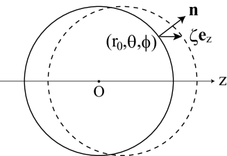
Figure 2: We draw a cross section including the $z$-axis. The bottom of the harmonic potential is fixed at the origin $O$. In the unperturbed state, the particle center is fixed at $O$ and the particle surface is represented by the solid circle. A point on the surface, with its spherical coordinates given by $(r_{0},\theta,\phi)$, moves when the particle is shifted; $r_{0}$ denotes the particle radius. A transient particle surface is drawn with the dashed circle, and the displacement vector of the point is given by $\zeta\bm{e}_{z}$. The unit normal vector $\bm{n}$ at the point remains unchanged in the particle motion. The dimensionless radial length is defined as $s\equiv r/r_{0}$.

We take the spherical polar coordinates $(r,\theta,\phi)$, locating the origin at the bottom of the harmonic potential imposed externally. The particle motion is assumed to be along the $z$-axis (polar axis); $\bm{e}_{z}$ denotes the unit vector in the $z$-direction (Fig. 2). We write $\zeta(t)$ for the $z$-coordinate of the particle center. The total force exerted on the particle by the mixture is along the $z$-axis; its $z$-component is denoted by ${\cal F}_{z}(t)$. The reversible dynamics of the particle is given by

$$m{d^{2}\over dt^{2}}\zeta(t)={{\cal F}}_{z}(t)-m\omega_{0}^{2}\zeta(t)$$ (14)

instead of Eq. (3). We should calculate ${{\cal F}}_{z}$ from the fields of the mixture. Let us introduce the dimensionless parameter $\varepsilon$ so that we have

$$\zeta(t)=\varepsilon\zeta^{(1)}(t)\ .$$ (15)

Assuming $|\varepsilon|$ to be small, we calculate ${\cal F}_{z}$ up to the order of $\varepsilon$ in Sect. IV.5.

The equilibrium state occurring when the particle center is fixed at the origin is regarded as the reference state or the unperturbed state, where $\mu$ is homogeneous over a mixture region and so is ${p}$ because of Eq. (9) ofk . They are respectively given by the constants $\mu^{(0)}$ and ${p}^{(0)}$. The superscript ⁽⁰⁾ is used to indicate the field in the unperturbed state. Because of the symmetry of the unperturbed state, $\varphi^{(0)}$ depends only on $r\equiv|\bm{r}|$. As shown in Sect. IV.2, we find it to be given by

$$\varphi^{(0)}(r)=\varphi_{\infty}+{hr_{0}e^{(1-s)/s_{\rm c}}\over Ms(1+s_{\rm c}^{-1})}\ ,$$ (16)

where $s\equiv r/r_{0}$ is the dimensionless radial length. This result is obtained in Ref. holyst, and is used in Ref. ofk, . Up to the order of $\varepsilon$, we expand the fields as

$$\varphi(\bm{r},t)=\varphi^{(0)}(r)+\varepsilon\varphi^{(1)}(\bm{r},t)\ ,$$

$$\ \mu(\bm{r},t)=\mu^{(0)}+\varepsilon\mu^{(1)}(\bm{r},t)\ ,$$

$${p}(\bm{r},t)={p}^{(0)}+\varepsilon{p}^{(1)}(\bm{r},t)\ ,$$

$$\ {\rm and}\ \bm{v}(\bm{r},t)=\varepsilon\bm{v}^{(1)}(\bm{r},t)\ .$$ (17)

The field with the superscript ⁽¹⁾ is defined so that it becomes proportional to $\varepsilon$ after being multiplied by $\varepsilon$. The fields with the superscript ⁽¹⁾ in Eq. (17) vanish far from the particle.

We add an overtilde to the Fourier transform with respect to $t$, e.g.,

$${\tilde{p}}^{(1)}(\bm{r},\omega)={1\over 2\pi}\int_{-\infty}^{\infty}dt\ p^{(1)}(\bm{r},t)e^{i\omega t}\ .$$ (18)

Let $(r,\theta,\phi)$ be the components of the positional vector $\bm{r}$ in the mixture. Using a spherical harmonics $Y_{10}(\theta)=\sqrt{3/(4\pi)}\cos{\theta}$, because of the symmetry of the state, we can assume

$${\tilde{p}}^{(1)}(\bm{r},\omega)=p_{10}(r,\omega)Y_{10}(\theta)\ ,$$ (19)

whereby the coefficient function $p_{10}$ is defined. Similarly, we introduce the coefficient functions for the Fourier transforms of the other mixture fields at the order of $\varepsilon$. From Eqs. (6), (7), (9), and (10), we can obtain a set of simultaneous equations with respect to these coefficient functions. The equations are given by Eqs. (41), (44), and (56) in Sect. IV; we assume the preferential attraction to be weak to solve them approximately. Before describing our calculation procedure, we show the result in the next section.

III Result

We define $\Xi(s)$ so that ${\varphi^{(0)}}^{\prime}(r)$ equals $r_{0}\Xi(s){\varphi^{(0)}}^{\prime\prime}(r_{0})$, i.e.,

$$\Xi(s)=-{s+s_{\rm c}\over s^{2}\kappa\left(1+s_{\rm c}\right)}e^{(1-s)/s_{\rm c}}\ ,$$ (20)

where we use

$$\kappa\equiv 2+{1\over s_{\rm c}\left(1+s_{\rm c}\right)}\ .$$ (21)

We have ${\varphi^{(0)}}^{\prime\prime}(r_{0})=h\kappa/(Mr_{0})$ because of Eq. (16). Let us define the positive dimensionless parameter $\Lambda$ so that we have

$$\Lambda^{2}\equiv{h^{2}\kappa\over\rho\omega^{2}r_{0}^{2}M}\ .$$ (22)

The calculation in Sect. IV.5 supposes $\Lambda^{2}\ll 1$, which holds when $h^{2}$ is sufficiently small, i.e., when the preferential attraction is sufficiently weak. This inequality condition is paraphrased more conveniently at the end of Sect. IV.5.

After the calculation shown in Sect. IV, we can rewrite Eq. (14) as

$$\left(m+{2\pi\rho r_{0}^{3}\over 3}\right){d^{2}\zeta\over dt^{2}}=-\left\{m\omega_{0}^{2}\left[1+\lambda^{2}D(s_{\rm c})\right]\right\}\zeta$$ (23)

up to the order of $\varepsilon$. This represents the small oscillation of the particle about the equilibrium point. Here, $\lambda$ is a dimensionless parameter defined as $h\sqrt{6\pi r_{0}/(Mm)}/\omega_{0}$; $D$ is defined as

$$D(s_{\rm c})\equiv 2\kappa^{2}\int_{1}^{\infty}ds\ {\Xi(s)^{2}\over s^{6}}\ ,$$ (24)

which is plotted in Fig. 3 with the aid of the software Mathematica (Wolfram Research). The second term in the parentheses on the left-hand side (lhs) of Eq. (23) represents the induced mass, which equals half the mass of the displaced mixture, as stated below Eq. (1). The term involving $\lambda^{2}$ on the right-hand side (rhs) represents the additional restoring force due to the deformed adsorption layer. We can derive $D(s_{\rm c})\approx s_{\rm c}$ for a small $s_{\rm c}$, as shown by Eq. (91). In agreement with this, the numerical results in Fig. 3 for a small $s_{\rm c}$ have the slope of about unity.

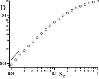
Figure 3: Circles represent $D(s_{\rm c})$ calculated from Eq. (24). The slope of unity is shown by the short line for reference.

From Eq. (23), we apply the equipartition theorem to obtain

$$\langle\zeta^{2}\rangle=k_{\rm B}T\left[m\omega_{0}^{2}+{6\pi h^{2}r_{0}\over M}D(s_{\rm c})\right]^{-1}\ ,$$ (25)

which gives the mean square displacement of the particle. The sum in the braces of Eq. (25) is the same as the one in the brackets of Eq. (23). Comparing Eq. (25) with the first equation of Eq. (1), we find that the effect of the deformed adsorption layer is represented by the second term in the braces of Eq. (25), which comes from the additional restoring force. This term reduces the mean square displacement, i.e., it suppresses the fluctuation amplitude. The suppression effect is more marked as $h^{2}$ and $\xi_{\rm c}$ are larger. Then, the adsorption layer is also remarkable in its thickness and amplitude, considering Eq. (16).

IV Calculation procedure

Here, we describe the calculation procedure leading to Eq. (23), with some details being relegated to Appendix C. A similar procedure is taken in Ref. pre, , where a fluid membrane fluctuating around a plane is studied. We have only to modify the procedure to consider the spherical surface of the particle in the present problem.

IV.1 Pressure tensor

The reversible part of the pressure tensor is given by Onukibook ; ofk

$$\Pi=\left(p-f+\mu\varphi-{M\over 2}\left|\nabla\varphi\right|^{2}\right)\bm{1}+M\nabla\varphi\nabla\varphi\ ,$$ (26)

where $\bm{1}$ denotes the isotropic tensor and $\mu$ is given by Eq. (7). In the above, the part other than $p\bm{1}$ is derived from the first term of Eq. (5), and $\varphi f^{\prime}-f$ gives the osmotic pressure deg . Because $\nabla\cdot\Pi$ equals $\nabla p+\varphi\nabla\mu$, we have Eq. (9). Let the local stress exerted on the particle by the ambient mixture be denoted by $\bm{F}(\bm{r}_{\rm s},t)$, where $\bm{r}_{\rm s}$ represents a point on the particle surface. We have

$$\bm{F}(\bm{r}_{\rm s},t)=-\Pi\cdot\bm{n}+\nabla_{\parallel}f_{\rm s}-{2f_{\rm s}\over r_{0}}\bm{n}\ .$$ (27)

Here, $\nabla_{\parallel}$ implies the projection of $\nabla$ on the tangent plane and $1/r_{0}$ gives the mean curvature of the particle surface. The last two terms above come from the stress due to the two-dimensional pressure $-f_{\rm s}$, as discussed in Appendix A of Ref. visc, . The tangential components of $\bm{F}$ vanish; the contribution from $M\nabla\varphi\nabla\varphi$ of Eq. (26) cancels with the tangential stress due to $f_{\rm s}$, as described in Appendix D of Ref. visc, . In fact, we use Eq. (8) to rewrite the rhs of Eq. (27) as

$$\left(-{p}+f+{M\over 2}|\nabla\varphi|^{2}-\mu\varphi-{h^{2}\over M}-{2f_{\rm s}\over r_{0}}\right)\bm{n}\ ,$$ (28)

which is evaluated immediately outside the boundary layer generated in the limit of zero viscosity. See the statement below Eq. (9).

IV.2 Profile in the unperturbed state

We write $\partial_{r}$ for the differentiation with respect to $r$, and $\partial_{r}^{2}$ for $\partial_{r}\partial_{r}$. As argued for a mixture in contact with a flat wall Cahn , Eq. (7) yields

$$f^{\prime}(\varphi^{(0)})-{M\over r}\partial_{r}^{2}r\varphi^{(0)}=\mu^{(0)}\ ,$$ (29)

while Eq. (8) yields

$$M{\partial\over\partial r}\varphi^{(0)}=-h\quad{\rm as}\ r\to r_{0}+\ .$$ (30)

Solving these equations, we arrive at Eq. (16). The equilibrium profile around a sphere was studied under conditions other than those considered here indekeu ; upton ; liu ; hanke .

IV.3 Equations at the order of $\varepsilon$

Suppose a point, $(r_{0},\theta,\phi)$, on the particle surface in the unperturbed state (Fig. 2). By the particle motion, its $z$-coordinate changes from $z_{0}\equiv r_{0}\cos{\theta}$ to $z_{0}+\zeta$. The slip boundary condition up to the order of $\varepsilon$ gives

$$\left.v_{r}^{(1)}\right|_{z_{0}}={d\zeta^{(1)}\over dt}\cos{\theta}\ ,$$ (31)

where the subscript $z_{0}$ means that the term is evaluated at the point on the surface in the unperturbed state, $(r_{0},\theta,\phi)$. Equation (8) is rewritten as

$$-h=\left.M\bm{n}\cdot\nabla\varphi\right|_{z_{0}+\zeta}\ ,$$ (32)

where the subscript $z_{0}+\zeta$ means that the term is evaluated at the point on the surface of the shifted particle. The unit normal vector $\bm{n}$ remains the same during the particle motion (Fig. 2). We have

$$\left.\varphi\right|_{z_{0}+\zeta}=\left.\varphi^{(0)}\right|_{z_{0}+\zeta}+\left.\varepsilon\varphi^{(1)}\right|_{z_{0}}+{\cal O}(\varepsilon^{2})\ ,$$ (33)

where ${\cal O}(\varepsilon^{2})$ means the terms whose quotient divided by $\varepsilon^{2}$ remains finite in the limit of $\varepsilon\to 0$. The first term on the rhs above is rewritten as

$$\varphi^{(0)}(r_{0})+\left.\zeta{\partial\over\partial z}\varphi^{(0)}(r)\right|_{z_{0}}\ .$$ (34)

Considering Eq. (30), we use these three equations to obtain

$$\left.{\partial\over\partial r}\varphi^{(1)}\right|_{z_{0}}=-\zeta^{(1)}{\varphi^{(0)}}^{\prime\prime}(r_{0})\cos{\theta}\ .$$ (35)

Using Eqs. (29), (30), and (35), we rewrite Eq. (28) so that it is evaluated on the particle surface in the unperturbed state. Integrating the result over the surface, we obtain up to the order of $\varepsilon$

$${\cal F}_{z}=2\varepsilon\pi r_{0}^{2}\int_{0}^{\pi}d\theta\ \sin{\theta}\cos{\theta}\left[-p^{(1)}-\mu^{(1)}\varphi^{(0)}\right.$$

$$\left.+\left(\varphi^{(1)}-{h\over M}\zeta^{(1)}\cos{\theta}\right)\left({2h\over r_{0}}+{M\over r_{0}}\partial_{r}^{2}r{\varphi^{(0)}}\right)\right]\ ,$$ (36)

where the integrand is evaluated at $(r_{0},\theta,\phi)$. We define ${\cal F}_{z}^{(1)}$ so that ${\cal F}_{z}$ equals $\varepsilon{\cal F}_{z}^{(1)}$ up to the order of $\varepsilon$.

As in Eq. (19), we define the coefficient functions $Q_{10}$ and $G_{10}$ so that we have

$${\tilde{\mu}}^{(1)}(\bm{r},\omega)=Q_{10}(r,\omega)Y_{10}(\theta)$$

$${\rm and}\ {\tilde{\varphi}}^{(1)}(\bm{r},\omega)=G_{10}(r,\omega)Y_{10}(\theta)\ .$$ (37)

We use the vector spherical harmonics

$$\bm{P}_{10}(\theta,\phi)=\bm{e}_{r}Y_{10}\ {\rm and}\$$ (38)

$$\bm{B}_{10}(\theta,\phi)={1\over\sqrt{2}}\bm{e}_{\theta}{\partial\over\partial\theta}Y_{10}(\theta)\ ,$$ (39)

where $\bm{e}_{r}$ and $\bm{e}_{\theta}$ denote the unit vectors tangent to the coordinate line of $r$ and curve of $\theta$, respectively. As in Ref. ofk, , we can assume

$${\tilde{\bm{v}}}^{(1)}(\bm{r},\omega)=R_{10}(r,\omega)\bm{P}_{10}(\theta,\phi)+T_{10}(r,\omega)\bm{B}_{10}(\theta,\phi)\ ,$$ (40)

where the functions $R_{10}$ and $T_{10}$ are introduced.

Below, we derive the equations to be satisfied by the coefficient functions. Using Eqs. (19) and (40) in Eqs. (6) and (9), we obtain Eqs. (79)–(81), which generate

$${r^{2}\over 2}\partial_{r}^{2}R_{10}+2r\partial_{r}R_{10}={{\varphi^{(0)}}^{\prime}Q_{10}\over i\rho\omega}\ .$$ (41)

We introduce $\zeta_{10}$ so that we have

$${\tilde{\zeta}}^{(1)}(\omega)=\sqrt{{3\over 4\pi}}\zeta_{10}(\omega)\ .$$ (42)

Equation (31) yields

$$\left.R_{10}\right|_{z_{0}}=-i\omega\zeta_{10}\ ,$$ (43)

and $R_{10}$ vanishes far from the particle, as stated below Eq. (17). If $h$ vanishes, $\mu$ and $\varphi$ are constant; the constant solutions satisfy Eqs. (7), (8), (10), and (11) together with the boundary conditions far from the particle. Then, we find $R_{10}(r,\omega)=-i\omega\zeta_{10}r_{0}^{3}/r^{3}$ from Eq. (41) and the boundary conditions. Thus, otherwise, $R_{10}$ is given by the sum of this solution for $h=0$ and terms dependent on $h$.

Equation (10) yields

$$-i\omega G_{10}=-R_{10}{\varphi^{(0)}}^{\prime}+L\left(\partial_{r}^{2}+{2\over r}\partial_{r}-{2\over r^{2}}\right)Q_{10}\ .$$ (44)

If we assume $L$ to vanish from the beginning, Eq. (44) gives

$$i\omega G_{10}=R_{10}{\varphi^{(0)}}^{\prime}\ ,$$ (45)

which is differentiated with respect to $r$ to give ${\varphi^{(0)}}^{\prime}\partial_{r}R_{10}=0$ at $r\to r_{0}+$ with the aid of Eq. (35). Thus, then, we have $\partial_{r}R_{10}\to 0$ at $r\to r_{0}+$ for $h\neq 0$. It is impossible to impose this boundary condition for any nonzero $h$ because Eq. (41) has two other boundary conditions mentioned at and below Eq. (43). This contradiction means that, if $h$ does not vanish, Eq. (45) is valid only outside the boundary layer. Then, even when $L$ approaches zero, the second term on the rhs of Eq. (44) cannot be neglected inside the boundary layer because of the steep change in $Q_{10}$. A similar problem occurs in the study of a fluid membrane fluctuating around a plane pre ; the thickness of the boundary layer of the chemical potential vanishes in the limit of $L\to 0+$. The solution outside the boundary layer is called the outer solution bender . Equation (45) thus holds only if $G_{10}$ and $R_{10}$ are replaced by their respective outer solutions.

IV.4 Nondimensionalization

We introduce the dimensionless fields

$${\cal G}(s,\omega)\equiv{MG_{10}(r,\omega)\over h\kappa\zeta_{10}(\omega)}$$

$${\rm and}\ {\cal Q}(s,\omega)\equiv{r_{0}^{2}Q_{10}(r,\omega)\over h\zeta_{10}(\omega)}\ ,$$ (46)

which do not diverge when $h$ vanishes because of the statement below Eq. (43). Hereafter, we sometimes write ${\cal G}$ or ${\cal G}(s)$ for ${\cal G}(s,\omega)$, and ${\cal G}^{\prime}$ for $\partial_{s}{\cal G}$. These ways of writing are also applied for other dimensionless functions. From Eq. (35) and the statement below Eq. (17), we have

$${\cal G}^{\prime}\to-1\ {\rm as}\ s\to 1+\ {\rm and}\quad{\cal G}\to 0\ {\rm as}\ s\to\infty\ .$$ (47)

From Eq. (11) and the statement below Eq. (17), we have

$${\cal Q}^{\prime}\to 0\ {\rm as}\ s\to 1+\ {\rm and}\quad{\cal Q}\to 0\ {\rm as}\ s\to\infty\ .$$ (48)

We write ${\cal G}_{\rm out}$ and ${\cal Q}_{\rm out}$ for the outer solutions of ${\cal G}$ and ${\cal Q}$, respectively. Equation (45) gives the first of our key equations,

$${\cal G}_{\rm out}=-\Xi{\cal R}_{\rm out}\ ,$$ (49)

where ${\cal R}_{\rm out}$ denotes the outer solution of

$${\cal R}(s,\omega)\equiv{iR_{10}(r,\omega)\over\omega\zeta_{10}(\omega)}\ .$$ (50)

We rewrite Eq. (41) as

$$\left({s^{2}\over 2}\partial_{s}^{2}+2s\partial_{s}\right){\cal R}=\Lambda^{2}\Xi{\cal Q}\ .$$ (51)

Equation (43) and the statement below it give

$${\cal R}\to 1\ {\rm as}\ s\to 1+\ {\rm and}\quad{\cal R}\to 0\ {\rm as}\ s\to\infty\ .$$ (52)

Applying the method of variation of parameters to Eqs. (51) and (52), we obtain the second of our key equations,

$${\cal R}(s)=s^{-3}+{2\over 3}\Lambda^{2}\int_{1}^{\infty}d\sigma\Gamma_{\rm R}(s,\sigma)\Xi(\sigma){\cal Q}(\sigma)\ ,$$ (53)

where the kernel is defined by

$$\Gamma_{\rm R}(s,\sigma)=\left\{\begin{array}[]{ll}s^{-3}\sigma^{-1}\left(1-\sigma^{3}\right)&{\rm for}\ \sigma<s\\ s^{-3}\sigma^{-1}\left(1-s^{3}\right)&{\rm for}\ s\leq\sigma\end{array}\right.\ .$$ (54)

Picking up terms at the order of $\varepsilon$ of Eq. (7) yields

$$-\mu^{(1)}=\left(M\Delta-a\right)\varphi^{(1)}\ .$$ (55)

Substituting Eq. (37) into the Fourier transform of Eq. (55), we obtain

$$-{\cal Q}=\kappa\left(\partial_{s}^{2}+{2\over s}\partial_{s}-{2\over s^{2}}-{1\over s_{\rm c}^{2}}\right){\cal G}$$ (56)

with the aid of Eq. (46). Applying the method of variation of parameters to Eq. (56), we use the second condition of Eq. (47) to obtain the last of our key equations,

$${\cal G}(s)={\cal G}^{\prime}(1+)\Xi(s)+{s_{\rm c}\over\kappa\sqrt{s}}\int_{1}^{\infty}d\sigma\ \sqrt{\sigma}\Gamma_{\rm G}(s,\sigma){\cal Q}(\sigma)\ ,$$ (57)

where the kernel $\Gamma_{\rm G}$ is defined by Eq. (84) and ${\cal G}^{\prime}(1+)$ denotes ${\cal G}^{\prime}(s)$ at $s\to 1+$. Because of the first condition of Eq. (47), we can substitute $-1$ into ${\cal G}^{\prime}(1+)$ above.

We can define ${\cal Q}_{\rm out}(s,\omega)$ for $s>1$ in the limit of $L\to 0+$. Subtracting it from ${\cal Q}(s,\omega)$, we define ${\cal Q}_{\rm in}(s,\omega)$ as the difference. It vanishes outside the boundary layer, but cannot be neglected in the following integral. Assuming that $s$ lies outside the boundary layer in Eq. (57), we obtain

$${\cal G}_{\rm out}(s)=-\Xi(s)\left[1+{1\over\kappa}\int_{1}^{\infty}d\sigma\ {\cal Q}_{\rm in}(\sigma)\right]$$

$$\quad+{s_{\rm c}\over\kappa\sqrt{s}}\int_{1}^{\infty}d\sigma\ \sqrt{\sigma}\Gamma_{\rm G}(s,\sigma){\cal Q}_{\rm out}(\sigma)$$ (58)

in the limit of $L\to 0+$.

IV.5 Weak preferential attraction

Assuming $\Lambda^{2}\ll 1$, we use the key equations in the preceding subsection to calculate ${\cal F}_{z}$ in Eq. (14). To do so, we obtain ${\cal Q}$ up to the order of $\Lambda$ and use the result in Eq. (53) to calculate ${\cal R}$ up to the order of $\Lambda^{3}$. To begin with, from Eqs. (49) and (53), we derive

$${\cal G}_{\rm out}(s)=-{\Xi(s)\over s^{3}}+{\cal O}(\Lambda^{2})\ ,$$ (59)

which leads to

$${\cal G}^{\prime}_{\rm out}(1+)=-1-{3\over\kappa}+{\cal O}(\Lambda^{2})\ .$$ (60)

Equation (56) remains valid if ${\cal Q}$ and ${\cal G}$ are respectively replaced by ${\cal Q}_{\rm out}$ and ${\cal G}_{\rm out}$. Thus, we can do the same replacement in Eq. (57) although ${\cal G}_{\rm out}^{\prime}(1+)$ is given not by the first condition of Eq. (47) but by Eq. (60). Thus, in the limit of $L\to 0+$, we find com

$${s_{\rm c}\over\kappa\sqrt{s}}\int_{1}^{\infty}d\sigma\ \sqrt{\sigma}\Gamma_{\rm G}(s,\sigma){\cal Q}_{\rm out}(\sigma)$$

$$\quad=-s^{-3}\Xi(s)+\left(1+{3\over\kappa}\right)\Xi(s)+{\cal O}(\Lambda^{2})\ .$$ (61)

Substituting Eq. (61) into Eq. (58), we use Eq. (59) to obtain

$$\int_{0}^{\infty}d\sigma\ {\cal Q}_{\rm in}(\sigma)=3+{\cal O}(\Lambda^{2})\ .$$ (62)

At Eq. (86), ${\cal Q}_{\rm out}$ is calculated up to the order of $\Lambda$.

Taking the limit of $s\to 1+$ in Eq. (57), we use Eqs. (61) and (62) to find

$${\cal G}(1+)={1\over\kappa}+{\cal O}(\Lambda^{2})$$ (63)

with the aid of Eqs. (20) and (21). Thus, up to the order of $\Lambda$, the difference in the first parentheses of Eq. (36) vanishes. We can rewrite the first two terms in the braces of Eq. (36) by using Eqs. (79) and (81). Using this result and Eq. (52), we obtain

$${\tilde{\cal F}}_{z}^{(1)}(\omega)=-{2\pi\rho\omega^{2}r_{0}^{3}\over 3}\left[2+{\cal R}^{\prime}(1+)+{\cal O}(\Lambda^{4})\right]{\tilde{\zeta}}^{(1)}(\omega)\ .$$ (64)

As shown in Appendix C, we can utilize Eqs. (53), (62), and (86) to obtain

$${\cal R}^{\prime}(1+)=-3+18\Lambda^{2}\kappa\int_{1}^{\infty}ds\ {\Xi(s)^{2}\over s^{6}}+{\cal O}(\Lambda^{4})\ .$$ (65)

From Eqs. (14), (64), and (65), we can derive Eq. (23). In its braces, the terms of $O(\lambda^{4})$ are neglected.

We can calculate ${\varphi}^{(1)}$ approximately from the first term on the rhs of Eq. (59). Comparing the values of $\varphi$ at the two points on the $z$-axis immediately outside the particle, we find that, if $h$ is positive, the value at $z=r_{0}+\zeta$ is larger (smaller) than the value at $z=-r_{0}+\zeta$ when $\zeta$ is positive (negative). Thus, within the approximation, the local difference of the mass density of the disliked component subtracted from the mass density of the preferred component is larger on the front side of the moving particle than on the rear side. This situation is shown by Fig. 1(b) if we regard the gray scale as representing the deviation of the local difference from its value far from the particle.

It is usual that the specific gravity of the particle is about unity. In Eq. (3), the normal-mode frequency is thus about $\sqrt{2/3}\omega_{0}$ because of $m_{\rm ind}\approx m/2$. The Fourier transform of Eq. (23) determines the normal-mode frequency $\omega$ changed by the deformed adsorption layer. Because the change is small in our perturbative calculation, we can use $\sqrt{2/3}\omega_{0}$ instead of $\omega$ in evaluating Eq. (22) approximately. As mentioned in the fourth paragraph of Sect. I, $s_{\rm c}=\xi_{\rm c}/r_{0}\ll 1$ is assumed in our hydrodynamics, which leads to $\kappa\approx 1$ in Eq. (21). Thus, the condition $\Lambda^{2}\ll 1$ can be identified with $\lambda^{2}/3\ll 1$, where $\lambda$ is defined above Eq. (24). Thus, assuming $\Lambda^{2}\ll 1$ amounts to assuming a sufficiently weak surface field. We also find that our approximate calculation supposes a sufficiently large $\omega_{0}^{2}$. This is reasonable, considering that the deformation of the adsorption layer becomes smaller as the particle moves more slowly.

V Discussion

The deformed adsorption layer generates the additional restoring force of a trapped particle, as shown in Eq. (23), and thus its mean square displacement is reduced, as shown by Eq. (25). No additional force can be calculated if we regard the ambient mixture as a simple bath and disregard its hydrodynamic effect, as shown in Appendix B. The suppression effect of the adsorption layer on the fluctuation amplitude was also pointed out for a fluid membrane immersed in a near-critical binary fluid mixture pre ; preprint . The relevance of the hydrodynamic effect is less distinct around the membrane, however, because incorrect but nonzero additional force can be calculated for the membrane even without the hydrodynamic effect being considered, as mentioned at the end of Appendix B.

For example, suppose a mixture of nitroethane and 3-methylpentane, which has $T_{\rm c}=300$ K. The mixture has $\xi_{\rm c}\approx 10$ nm for $T-T_{\rm c}\approx 0.3$ K at the critical composition iwan . On the basis of the discussion in Ref. liu, , $h\approx 10^{-6}$ m³/s² is estimated in Ref. pre, for a glass surface and an organic mixture, between which a strong hydrogen bonding is formed. Supposing a surface not forming the hydrogen bonding so strongly, we use $h=10^{-7}$ m³/s². The coefficient of the square gradient term in the free-energy density is sometimes called the influence parameter rowl ; poser . This parameter can be defined in general for each pair of components, $A$-$A$, $B$-$B$, and $A$-$B$, where $A$ and $B$ represent the kinds of the two components. The coefficient $M$ is for the last pair, which can be regarded roughly as the geometric mean of the parameters for the first two pairs aiche . We cannot find out the data for the influence parameters of the mixture mentioned above. Judging from the data for the pure fluid of alkane, we use $M=10^{-16}$ m⁷/(s²kg) vdwexp . For these parameter values, as discussed below Eq. (72), a correlation length longer than about $10$ nm cannot be assumed in the regime of the Gaussian model.

The spring constant of the optical tweezers typically ranges from $10^{-3}$ to $10^{-6}$ kg/s² daniel . Let us assume it to be $m\omega_{0}^{2}=4.14\times 10^{-4}$ kg/s², which leads to $\langle\zeta^{2}\rangle\approx 10$ nm² in Eq. (1) without the ambient near-criticality being assumed. Suppose a particle having $r_{0}=100$ nm with the specific gravity being about unity. We have $s_{\rm c}=0.1$ for the value of $\xi_{\rm c}$ mentioned above. As mentioned in the last paragraph of Sect. IV.5, our formulation supposes $\xi_{\rm c}\ll r_{0}$, i.e., $s_{\rm c}\ll 1$, which is satisfied by the values above. The prefactor of $D$ in Eq. (25) is calculated as $6\pi h^{2}r_{0}/M\approx 2\times 10^{-4}$ kg/s². Thus, we have $\lambda^{2}\approx 0.48$, which satisfies the condition for the weak preferential attraction, mentioned at the end of Sect. IV.5. According to Eq. (25), $\langle\zeta^{2}\rangle$ is reduced to about $9.5$ nm² by the deformed adsorption layer. Its square root is much smaller than $r_{0}$, which justifies the assumption of a small amplitude of the particle fluctuation. The change in $\langle\zeta^{2}\rangle$ from $10$ to $9.5$ nm² can be expected to be measured by means of the recent experimental technique, mentioned in Sect. I, although the increased turbidity in the near-critical mixture may make the measurement more delicate. The prefactor of $D$ contains $h^{2}/M$, while Eq. (16) contains a factor $h/M$. Thus, we can determine the material constants, $h$ and $M$, experimentally from the suppression effect and unperturbed profile if they are both measured. Similar discussions are found in Refs. pre, and relax, .

It is assumed in our calculation leading to the result, Eq. (25), that a rigid sphere fluctuates with a small amplitude, that the mixture in the homogeneous phase is not too close to the critical point, and that the particle surface attracts one component weakly. Thus, we cannot apply the result beyond the parameter range generating a weak suppression effect. A larger suppression effect may be observed experimentally in a setup with some appropriate parameter values. Predicting this requires future theoretical or numerical studies not requiring the assumptions above. The present study can be a guide for them. We also assume the preferential attraction to be caused by a short-range interaction and to be represented only by the surface field. How the suppression effect is altered without these assumptions also remains to be studied. We assume a particle size much larger than the correlation length to use the hydrodynamics based on the coarse-grained free-energy functional. For a smaller particle, the critical concentration fluctuation of the mixture would influence the particle motion, and a procedure other than that used in the present study should be taken. This is also a future problem.

Appendix A Validity of the Gaussian model

In cases more general than considered in the Gaussian model, we can use the renormalized local functional theory, which was proposed by Okamoto and Onuki JCP ; PRE . They studied the universal properties of a near-critical binary fluid mixture between two parallel walls or two spheres. Here, we assume that the mixture has the critical composition far from the solid surface. The order parameter and correlation length are not homogeneous and are respectively denoted by $\psi(\bm{r})\equiv\varphi(\bm{r})-\varphi_{\infty}$ and $\xi(\bm{r})$. The correlation length far from the surface, denoted by $\xi_{\infty}$, is asymptotically equal to $\xi_{0}\tau^{-\nu}$ as $\tau$ approaches zero, where $\xi_{0}$ is a nonuniversal constant, $\tau\equiv\left(T-T_{\rm c}\right)/T_{\rm c}$ is assumed to be positive, and the critical exponent $\nu$ is about $0.627$ for the binary fluid mixture. We also use the critical exponents $\gamma\approx 1.239$ and $\eta\approx 0.024$. In the Gaussian model, $\xi_{\rm c}$ is regarded as $\xi_{\infty}$.

Subtracting the volume integral of $\mu^{(0)}\varphi$ over $C^{\rm e}$ from Eq. (5) with Eq. (12) gives the free-energy functional for the open system in the Gaussian model. Apart from an additional constant, the corresponding functional in the renormalized local functional theory can be obtained by replacing $M$ and $f-\mu^{(0)}\varphi$ respectively by $C$ and $f_{\rm R}$ defined below. The coefficient $C$ depends on $\psi$ as

$$C(\psi)\equiv k_{\rm B}T_{\rm c}C_{1}w^{-\eta\nu}\ ,$$ (66)

where $C_{1}$ is a nonuniversal constant and $w$ is defined by $w\equiv\xi_{0}^{1/\nu}\xi^{-1/\nu}$, while $f_{\rm R}$ is given by

$$f_{\rm R}(\psi)\equiv k_{\rm B}T_{\rm c}\left({1\over 2}C_{1}\xi_{0}^{-2}w^{\gamma-1}\tau\psi^{2}\right.$$

$$\qquad\qquad\left.+{1\over 4}C_{1}^{2}u^{*}\xi_{0}^{-\epsilon}w^{\gamma-2\beta}\psi^{4}\right)\ ,$$ (67)

as a result of the $\epsilon$-expansion. In later numerical calculations, we use $\epsilon=1$ and approximate the constant $u^{*}$ to be $2\pi^{2}/9$. Equation (67) is found to be the same as Eq. (3.5) of Ref. JCP, with the aid of the scaling law $\left(\epsilon-2\eta\right)\nu=\gamma-2\beta$. Here, because the critical composition is assumed far from the surface, $\mu_{\infty}$ in Ref. JCP, vanishes.

The free-energy functional after the replacement above is the one renormalized up to the local correlation length without rescaling, as in the exact renormalization group theory litim . Thus, we can apply the mean-field theory to calculate $\xi$ at each locus, which leads to

$$w=\tau+C_{2}w^{1-2\beta}\psi^{2}\ ,$$ (68)

where we use $C_{2}\equiv 3u^{*}C_{1}\xi_{0}^{2-\epsilon}$. These equations can be found in Ref. JCP, ; see Eqs. (3.9) and (3.11) and the statement below its Eq. (3.16) in this reference. Defining $U\equiv w/\tau$ and

$$s\equiv C_{2}U^{1-2\beta}\tau^{-2\beta}\psi^{2}\ ,$$ (69)

we rewrite Eq. (68) as $U=1+s$. Here, $s$ is defined unlike in the text. Equation (67) is rewritten as

$$f_{\rm R}(\psi)={k_{B}T_{\rm c}C_{1}\tau^{2\beta+\gamma}\over 2C_{2}\xi_{0}^{2}}U^{2\beta+\gamma-2}\left(s+{s^{2}\over 6}\right)\ .$$ (70)

When only values of $s$ much smaller than unity are significant, we can neglect $s^{2}/6$ above to use $C(\psi)\psi^{2}/(2\xi_{\infty}^{2})$ as $f_{\rm R}(\psi)$ approximately. Then, regarding $C$ and $\xi_{\infty}$ as $M$ and $\xi_{\rm c}$, respectively, we find that the Gaussian model is valid.

By using the free-energy functional introduced above, let us consider the range of $\xi_{\rm c}$ validating the Gaussian model. To do so, limiting our discussion to cases of $\xi_{\rm c}\ll r_{0}$, we can assume the mixture to occupy the semi-infinite space bounded by a flat surface. Here, we take the $z$-axis so that the mixture lies in $z>0$. The order parameter is not rescaled in the renormalized local functional theory, and thus $f_{\rm s}$ remains unchanged in the renormalization process. As discussed in Sect. IIB of Ref. JCP, , the order-parameter profile at equilibrium is obtained by minimizing the free-energy functional because it is renormalized up to the local correlation length. Writing ${\bar{\psi}}(z)$ for the profile, we obtain

$$C({\bar{\psi}}(z))\left|{d{\bar{\psi}}(z)\over dz}\right|^{2}=2f_{\rm R}({\bar{\psi}}(z))$$ (71)

for $z>0$, and

$$C({\bar{\psi}(z)}){d{\bar{\psi}}(z)\over dz}=-h$$ (72)

as $z\to 0+$. In the limit of $z\to\infty$, ${\bar{\psi}}(z)$ vanishes. Let us write ${\bar{s}}(z)$ for the variable $s$ determined by this profile ${\bar{\psi}}(z)$, and ${\bar{s}}(0+)$ for ${\bar{s}}(z)$ in the limit of $z\to 0+$. We can derive the differential equation with respect to ${\bar{s}}(z)$ from Eqs. (69)–(71), and derive the algebraic equation with respect to ${\bar{s}}(0+)$ from Eqs. (70)–(72). The former shows that ${\bar{s}}(z)$ decreases monotonically to zero as $z$ increases from zero to infinity preprint . Using the material constants mentioned in Sect. V and $\xi_{0}=0.23$ nm for the mixture iwan , we numerically solve the latter to obtain Fig. 4(a). We find that ${\bar{s}}(0+)$ is much smaller than unity when $\tau$ is larger than about $2\times 10^{-3}$. Then, we have ${\bar{s}}(z)\ll 1$ for any $z>0$ and the Gaussian model is valid. Calculating the correlation length immediately near the surface $\xi(0+)$ from ${\bar{s}}(0+)$, we plot the results in Fig. 4(b), where $\xi_{\infty}$ is also plotted for comparison. These lengths turn out to agree only when the Gaussian model is valid, and then $\xi_{\infty}$ (or $\xi_{\rm c}$) is smaller than about $10$ nm. As $\tau$ is smaller, $\xi(0+)$ reaches a plateau. This is because the surface field prevents the mixture near the surface from approaching the critical point. The Gaussian model cannot describe the separation of $\xi(0+)$ and $\xi_{\infty}$.

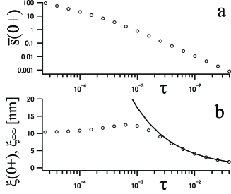
Figure 4: (a) We calculate ${\bar{s}}(0+)$, i.e., $\lim_{z\to 0+}{\bar{s}}(z)$, from Eqs. (69) and (72). (b) Circles represent $\xi(0+)$, while the solid curve represents $\xi_{\infty}$.

Below, we briefly show that the procedure mentioned above properly yields the well-known universal profile near the flat surface. Details can be found in Ref. preprint, , where the undulation amplitude of a fluid membrane is studied. When $\tau$ decreases beyond the regime of the Gaussian model, ${\bar{s}}(0+)$ is much larger than unity. Then, we have ${\bar{s}}(z)\gg 1$ up to a positive $z$. In this spatial region, Eqs. (69)–(71) lead to ${\bar{\psi}}^{\prime}\approx-\left({\bar{s}}\tau\right)^{\beta+\nu}/\left(\sqrt{6C_{2}}\xi_{0}\right)$ when $h$ is positive. Noting $\left({\bar{s}}\tau\right)^{\beta}\approx\sqrt{C_{2}}{\bar{\psi}}$, we find

$${\bar{\psi}}(z)\approx{1\over\sqrt{C_{2}}}\left[{\sqrt{6}\beta\xi_{0}\over\nu\left(z+l_{0}\right)}\right]^{\beta/\nu}\ ,$$ (73)

where $l_{0}\approx\sqrt{6}\beta\xi(0+)/\nu$ is found with the aid of Eq. (72). We find that ${\bar{s}}(z)\gg 1$ is valid for $z\ll\xi_{\infty}$. For $z\gg\xi_{\infty}$, the profile is shown to exhibit the same exponential decay as shown in the Gaussian model. This is well known, as well as the profile of Eq. (73) rudjas ; diehl94 ; smdilan . When $\tau$ is sufficiently small, we have the region of $l_{0}\ll z\ll\xi_{\infty}$, where Eq. (73) can be regarded as

$${\bar{\psi}}(z)\propto\left({\xi_{0}\over z}\right)^{\beta/\nu}=\tau^{\beta}\left({z\over\xi_{\infty}}\right)^{-\beta/\nu}\ ,$$ (74)

which is consistent with the universal form diehl97 ; diehl94 ; smdilan ; smock . Equation (73) is the same as Eq. (2.15) of Ref. JCP, in the case of $\tau=0$ and ${\bar{\psi}}(\infty)=0$ because of the statement below Eq. (3.15) in this reference. In this case, the region of the exponential decay vanishes, and the critical adsorption occurs.

Assuming $f_{\rm s}(\varphi)$ to be a linear function with a finite surface field, we can derive the universal form of the order-parameter profile, Eq. (74), in terms of the renormalized local functional theory, where the rescaling is not performed unlike in the conventional renormalization group theory. Here, we neglect the surface enhancement, i.e., the negative of the coefficient of the second-order term in $f_{\rm s}$. This should amount to assuming its bare value to be positive in the conventional renormalization group theory, where the surface enhancement is measured from the value at the special transition occurring at $h=0$ (see Ref. diehl97, and Eq. (3.95) of Ref. diehl86, ). We think that nonzero surface enhancement should not remarkably change the result in the present study, where the preferential attraction is assumed to be sufficiently weak.

Appendix B Naive average based on Eq. (5)

Here, we calculate the mean square displacement by regarding the mixture as a heat and particle bath. This procedure is improper, but is shown for comparison with the procedure described in the text. The following calculation is parallel with the one in the Appendix of Ref. pre, . We define $\Omega_{\rm b}$ as the first term of Eq. (5) with $f$ replaced by $f-\mu^{(0)}\varphi$, and define $\Omega_{\rm s}$ as the second term. Their sum is denoted by $\Omega$, which is the free-energy functional for the open system mentioned in the second paragraph of Appendix A. Suppose that $\varphi$ and $\zeta$ deviate from $\varphi^{(0)}$ and zero, respectively. Below, the resultant deviations of $\Omega_{\rm b}$, $\Omega_{\rm s}$, and $\Omega$, denoted by $\delta\Omega_{\rm b}$, $\delta\Omega_{\rm s}$, and $\delta\Omega$, respectively, are calculated up to the second order with respect to $\varphi_{1}\equiv\varphi-\varphi^{(0)}$ and $\zeta$. We add the subscript _ζ to $C^{\rm e}$ and $\partial C$ to indicate their dependences on $\zeta$. We find $\delta\Omega_{\rm s}[\varphi_{1},\zeta]$ to be given by

$$\int_{\partial C_{\zeta}}dS\ f_{\rm s}(\varphi)-\int_{\partial C_{0}}dS\ f_{\rm s}(\varphi^{(0)})$$

$$=-{h\zeta^{2}\over 2}\int_{\partial C_{0}}dS\ {\partial^{2}\over\partial z^{2}}\varphi^{(0)}-h\int_{\partial C_{\zeta}}dS\ \varphi_{1}$$ (75)

with the aid of Eq. (30). Similarly, writing $\Phi^{(0)}$ for $\varphi^{(0)}-\varphi_{\infty}$, we find $\delta\Omega_{\rm b}[\varphi_{1},\zeta]$ to be given by

$$\int_{C^{{\rm e}}_{\zeta}}d\bm{r}\ \left(a\Phi^{(0)}+M\nabla\varphi^{(0)}\cdot\nabla\right)\varphi_{1}$$

$$-{\zeta^{2}\over 4}\int_{\partial C_{0}}dS\ \cos{\theta}{\partial\over\partial z}\left(a{\Phi^{(0)}}^{2}+M\left|\nabla\varphi^{(0)}\right|^{2}\right)$$

$$+{1\over 2}\int_{C^{\rm e}_{0}}d\bm{r}\ \left(a\varphi_{1}^{2}+M\left|\nabla\varphi_{1}\right|^{2}\right)\ ,$$ (76)

which can be rewritten with the aid of Eqs. (29) and (30). The sum of Eqs. (75) and (76) gives $\delta\Omega[\varphi_{1},\zeta]$, which is rewritten as

$${1\over 2}\int_{\partial C_{0}}dS\ \left[\zeta^{2}h{\varphi^{(0)}}^{\prime\prime}\cos^{2}{\theta}-2\zeta M{\varphi^{(0)}}^{\prime\prime}\varphi_{1}\cos{\theta}\right.$$

$$\left.-M\bm{n}\cdot\left(\varphi_{1}\nabla\varphi_{1}\right)\right]+{1\over 2}\int_{C^{\rm e}_{0}}d\bm{r}\ \left(a\varphi_{1}^{2}-M\varphi_{1}\Delta\varphi_{1}\right)$$

(77)

with the aid of Eq. (30). Here, we also note that the surface integral of $(1-3\cos^{2}{\theta})$ over $\partial C_{0}$ vanishes.

In this procedure, the probability density of $\varphi_{1}$ and $\zeta$ at equilibrium is proportional to the Boltzmann weight, $\exp{\left(-\delta\Omega^{+}/k_{\rm B}T\right)}$, where $\delta\Omega^{+}$ is defined as $m\omega_{0}^{2}\zeta^{2}/2+\delta\Omega$. Integrating this density with respect to $\varphi_{1}$ yields the probability density of $\zeta$, from which we can find its variance, i.e., the mean square displacement. Apart from a multiplication constant, we can obtain the result of this integration by replacing $\delta\Omega^{+}$ by the minimum of $\delta\Omega^{+}$ for a given $\zeta$ in the Boltzmann factor because the probability density considered here is a Gaussian distribution. We write $\varphi_{1}^{*}$ for $\varphi_{1}$ minimizing $\delta\Omega^{+}$, and thus $\delta\Omega$, for a given $\zeta$. The stationary condition of Eq. (77) with respect to $\varphi_{1}$ is found to be given by Eq. (55) with its lhs being put equal to zero and Eq. (35) if $\varphi^{(1)}$ and $\zeta^{(1)}$ are respectively replaced by $\varphi_{1}^{*}$ and $\zeta$. The condition is satisfied by

$$\varphi_{1}^{*}(\bm{r})=-\zeta{\varphi^{(0)}}^{\prime}(r)\cos{\theta}\ .$$ (78)

The time variable $t$ need not be specified in this procedure. Replacing $\varphi_{1}$ with $\varphi_{1}^{*}$ in Eq. (77), we find it to vanish. This means that the probability density of $\zeta$ is not changed by the ambient mixture, and that the mean square displacement remains the same as the first equation of Eq. (1). In this procedure, considering that the rhs of Eq. (78) equals $\varphi^{(0)}\left(r-\zeta\cos{\theta}\right)-\varphi^{(0)}(r)$ up to the order of $\zeta$, the profile of $\varphi$ for a given $\zeta$ is obtained by the translational shift of the profile of Fig. 1(a) and such a deformed adsorption layer as shown in Fig. 1(b) cannot be obtained. It is thus reasonable that no additional force exerted on the particle can be calculated by this improper procedure. This is in contrast to the corresponding result for a fluctuating fluid membrane. Even if the ambient mixture is regarded as a simple bath improperly, the adsorption layer around the membrane is deformed and nonzero additional force can be calculated although the result is different from the one obtained from the proper calculation with hydrodynamic consideration pre ; preprint .

Appendix C Some details in the calculation

Substituting Eq. (40) into Eq. (6) gives

$$T_{10}={1\over\sqrt{2}r}\partial_{r}\left(r^{2}R_{10}\right)\ .$$ (79)

Picking up the terms with the order of $\varepsilon$ from the $r$- and $\theta$-components of Eq. (9) and substituting Eqs. (19) and (40) into their Fourier transforms, we obtain

$$-i\omega\rho R_{10}=-\partial_{r}P_{10}-\varphi^{(0)}\partial_{r}Q_{10}$$ (80)

$${\rm and}\ {-i\omega\rho rT_{10}\over\sqrt{2}}=-P_{10}-\varphi^{(0)}Q_{10}\ .$$ (81)

These three equations give Eq. (41).

Below, $I_{3/2}$ and $K_{3/2}$ represent modified Bessel functions. Using ${\tilde{s}}\equiv s/s_{\rm c}$ and ${\tilde{\sigma}}\equiv\sigma/s_{\rm c}$, we define

$$\Gamma_{\rm Gc}(s,\sigma)\equiv-{\hat{w}}(s_{\rm c})K_{3/2}({\tilde{s}})K_{3/2}({\tilde{\sigma}}){\tilde{\sigma}}\ .$$ (82)

Here, we use

$${\hat{w}}(s_{\rm c})\equiv{2e^{1/s_{\rm c}}\left[2s_{\rm c}{\rm cosh}s_{\rm c}^{-1}-\left(2s_{\rm c}^{2}+1\right){\rm sinh}s_{\rm c}^{-1}\right]\over\pi\left(1+s_{\rm c}\right)\kappa}\ ,$$ (83)

which equals Eq. (4.10) of Ref. ofk, if its $\zeta_{\rm c}$ is replaced by $s_{\rm c}$. The kernel used in Eq. (57) is defined as

$$\Gamma_{\rm G}(s,\sigma)\equiv\left\{\begin{array}[]{ll}\Gamma_{\rm Gc}(s,\sigma)+K_{3/2}({\tilde{s}})I_{3/2}({\tilde{\sigma}}){\tilde{\sigma}}&{\rm if}\ \sigma<s\\ \Gamma_{\rm Gc}(s,\sigma)+I_{3/2}({\tilde{s}})K_{3/2}({\tilde{\sigma}}){\tilde{\sigma}}&{\rm if}\ s\leq\sigma\end{array}\right.\ ,$$ (84)

which is the same as Eq. (4.11) of Ref. ofk, . In deriving Eq. (57), we utilize the identity

$$K_{3/2}(s)I^{\prime}_{3/2}(s)-I_{3/2}(s)K^{\prime}_{3/2}(s)=s^{-1}\ ,$$ (85)

and rewrite $I_{3/2}$ and $K_{3/2}$ in terms of the hyperbolic functions.

Equation (56) remains valid if ${\cal Q}$ and ${\cal G}$ are replaced by their respective outer solutions. Substituting Eq. (59) into the resultant equation gives

$${\cal Q}_{\rm out}(s)=-{3\kappa\over s^{2}\Xi(s)}{d\over ds}{\Xi(s)^{2}\over s^{2}}+{\cal O}(\Lambda^{2})\ .$$ (86)

Here, we note that the rhs of Eq. (56) with ${\cal G}(s)$ replaced by $\Xi(s)$ vanishes, which is found by substituting Eq. (12) into Eq. (29) and differentiating the result with respect to $r$. Taking the limit of $s\to 1+$ of the derivative of Eq. (53) with respect to $s$, we use Eqs. (20), (21), and (62) to obtain

$${\cal R}^{\prime}(1+)=-3-2\Lambda^{2}\left[-{3\over\kappa}+\int_{1}^{\infty}ds\ {\Xi(s)\over s}{\cal Q}_{\rm out}(s)\right]\ .$$ (87)

Substituting Eq. (86) into Eq. (87), we obtain Eq. (65) with the aid of the integration by parts.

Substituting Eq. (20) into Eq. (24) yields

$$D(s_{\rm c})={s_{\rm c}^{3}\over\left(1+s_{\rm c}\right)^{2}}\left[{E_{8}(s_{\rm c})\over s_{\rm c}^{2}}+{2E_{9}(s_{\rm c})\over s_{\rm c}}+E_{10}(s_{\rm c})\right]\ ,$$ (88)

where we use

$$E_{n}(s_{\rm c})\equiv{2^{n}e^{2/s_{\rm c}}\over s_{\rm c}^{n}}\int_{2/s_{\rm c}}^{\infty}d\tau\ \tau^{-n}e^{-\tau}\ .$$ (89)

As $s_{\rm c}\to 0+$, we have

$$E_{n}(s_{\rm c})\sim 1-{n\over 2}s_{\rm c}+{n(n+1)\over 4}s_{\rm c}^{2}+{\cal O}(s_{\rm c}^{3})\ .$$ (90)

Equations (88) and (90) give the asymptotic relation

$$D(s_{\rm c})\sim s_{\rm c}-4s_{\rm c}^{2}+{\cal O}(s_{\rm c}^{3})\quad{\rm as}\ s_{\rm c}\to 0+\ .$$ (91)

References

- (1) B. Lukić, S. Jeney, C. Tischer, A. J. Kulik, L. Forró, and E.-L. Florin, Phys. Rev. Lett. 95, 160601 (2005).
- (2) T. Franosch, M. Grimm, M. Belushkin, F. M. Mor, G. Foffi, L. Forró, and S. Jeney, Nature 478, 85 (2011).
- (3) R. Huang, I. Chavez, K. M. Taute, B. Lukić, S. Jeney, M. Raizen, and E.-L. Florin, Nat. Phys. 7, 576 (2011).
- (4) M. Grimm, T. Franosch, and S. Jeney, Phys. Rev. E 86, 021912 (2012).
- (5) H. Lamb, Hydrodynamics, (Dover, New York, 1932) 6th ed., Sect. 92.
- (6) J. W. Cahn, J. Chem. Phys. 66, 3667 (1977).
- (7) M. N. Binder, in Phase Transition and Critical Phenomena VIII, ed. C. Domb and J. L. Lebowitz (Academic, London 1983).
- (8) R. Holyst and A. Poniewierski, Phys. Rev. B 36, 5628 (1987).
- (9) R. Kubo, M. Toda, and N. Hashitsume, Statistical Physics II (Springer, Berlin, 1991) Chap. 1.6.
- (10) Why the energy is determined uniquely is discussed around Eq. (77) of Ref. pre, .
- (11) A. Onuki, Phase Transition Dynamics (Cambridge University Press, Cambridge, England, 2002) Chaps. 4 and 6.
- (12) K. Kawasaki, Ann. Phys. (N. Y.) 61, 1 (1970).
- (13) P. C. Hohenberg and B. I. Halperin, Rev. Mod. Phys. 49, 435 (1977).
- (14) A. Furukawa, A. Gambassi, S. Dietrich, and H. Tanaka, Phys. Rev. Lett. 111, 055701 (2013).
- (15) Y. Fujitani, J. Phys. Soc. Jpn. 83, 024401 (2014); 83, 108001 (2014) [erratum].
- (16) Y. Fujitani, J. Phys. Soc. Jpn. 83, 084401 (2014).
- (17) Y. Fujitani, J. Phys. Soc. Jpn. 82, 124601 (2013); 83, 088001 (2014) [erratum].
- (18) R. Okamoto, Y. Fujitani, and S. Komura, J. Phys. Soc. Jpn. 82, 084003 (2013).
- (19) S. Yabunaka, R. Okamoto, and A. Onuki, Soft Matter 11 5738 (2015).
- (20) A. J. Bray and M. A. Moore, J. Phys. A: Math. Gen. 10, 1927 (1977).
- (21) W. H. Diehl, in Phase Transition and Critical Phenomena X, ed. C. Domb and J. L. Lebowitz (Academic, London 1986).
- (22) T. W. Burkhardt and H. W. Diehl, Phys. Rev. B 50, 3894 (1994).
- (23) W. H. Diehl, Int. J. Mod. Phys. B 11, 3503 (1997).
- (24) Y. Fujitani, Phys. Rev. E 91 042402 (2015).
- (25) H. W. Diehl and H. K. Janssen, Phys. Rev. A 45, 7145 (1992).
- (26) C. M. Bender and S. A. Orszag, Advanced Mathematical Methods for Scientists and Engineers (Springer, New York, 1999) Chaps. 1.5 and 9.2.
- (27) P. G. de Gennes, Scaling Concepts in Polymer Physics (Cornell Univ Press, Ithaca, 1979) Sect. III. 1. 3.
- (28) J. O. Indekeu, P. J. Upton, and J. M. Yeomans, Phys. Rev. Lett. 61, 2221 (1988).
- (29) P. J. Upton, J. O. Indekeu, and J. M. Yeomans, Phys. Rev. B 40, 666 (1989).
- (30) A. J. Liu and M. E. Fisher, Phys. Rev. A 40, 7202 (1989).
- (31) A. Hanke and S. Dietrich, Phys. Rev. E 59, 5081 (1999).
- (32) Substituting Eq. (86) into the lhs of Eq. (61) yields the rhs. This is an alternative way of deriving Eq. (61).
- (33) Y. Fujitani, J. Phys. Soc. Jpn. 86, 044602 (2017).
- (34) I. Iwanowski, K. Leluk, M. Rudowski, and U. Kaatze, J. Phys. Chem. A 110, 4313 (2006).
- (35) J. S. Rowlinson and B. Widom, Molecular Theory of Capillarity (Clarendon Press, UK, 1982), Chaps. 3, 4.6, and 9.1-2.
- (36) C. I. Poser and I. C. Sanchez, Macromolecules 14, 361 (1981).
- (37) B. S. Carey, L. E. Scriven, and H. T. Davis, AIChE J. 26 705 (1980).
- (38) P. M. W. Cornelisse, C. J. Peters and J. de Swaan Arons, Fluid Phase Equilib. 117, 312 (1996).
- (39) D. Riveline, J. Nanobiotechnol. 11, 51 (2012).
- (40) Y. Fujitani, Eur. Phys. J. E. 39, 31 (2016).
- (41) D. F. Litim, Phys. Rev. D, 64 105007 (2001); J. Berges, arXiv:hep-ph/9902419v1.
- (42) R. Okamoto and A. Onuki, J. Chem. Phys. 136, 114704 (2012).
- (43) R. Okamoto and A. Onuki, Phys. Rev. E 88, 022309 (2013).
- (44) J. Rudnick and D. Jasnow, Phys. Rev. Lett 48, 1059 (1982).
- (45) W. H. Diehl, Ber. Bunsenges, Phys. Chem. 98, 466 (1994).
- (46) M. Smock, H. W. Diehl, and D. P. Landau, Ber. Bunsenges, Phys. Chem. 98, 486 (1994).
- (47) H. W. Diehl and M. Smock, Phys. Rev. B 47, 5841 (1993); 48, 6740 (1993) [erratum].