The de Broglie-Bohm pilot-wave formulation of quantum theory allows the existence of physical states that violate the Born probability rule. Recent work has shown that in pilot-wave field theory on expanding space relaxation to the Born rule is suppressed for long-wavelength field modes, resulting in a large-scale power deficit $\xi(k)$ which for a radiation-dominated expansion is found to have an approximate inverse-tangent dependence on $k$ (assuming that the width of the initial distribution is smaller than the width of the initial Born-rule distribution and that the initial quantum states are evenly-weighted superpositions of energy states). In this paper we show that the functional form of $\xi(k)$ is robust under changes in the initial nonequilibrium distribution – subject to the limitation of a subquantum width – as well as under the addition of an inflationary era at the end of the radiation-dominated phase. In both cases the predicted deficit $\xi(k)$ remains an inverse-tangent function of $k$. Furthermore, with the inflationary phase the dependence of the fitting parameters on the number of superposed pre-inflationary energy states is comparable to that found previously. Our results indicate that, for the assumed broad class of initial conditions, an inverse-tangent power deficit is likely to be a fairly general and robust signature of quantum relaxation in the early universe.

1 Introduction

According to inflationary cosmology, the temperature anisotropies in the cosmic microwave background (CMB) were seeded by primordial quantum fluctuations [1, 2, 3]. Precision measurements of the CMB may therefore provide us with tests of the quantum Born probability rule at very early times [4, 5, 6, 7, 8, 9].

The de Broglie-Bohm pilot-wave formulation of quantum theory [10, 11, 12, 13, 14] provides a natural extension of the usual quantum formalism, in which corrections to the Born rule are possible. In pilot-wave theory, the Born rule is not fundamental but only describes a state of statistical equilibrium [15, 16, 17, 18, 19, 20, 4, 5, 21, 6, 22, 23].

One may consider a universe that begins in a state of ‘quantum nonequilibrium’, with non-Born rule probabilities [17, 18, 19, 4, 5, 6]. The dynamics of pilot-wave theory allows us to evolve such a state forward in time. Extensive numerical simulations have been performed for a free scalar field evolving on a radiation-dominated background [7, 8], with a view to applying the results to a cosmology with a radiation-dominated pre-inflationary phase [24, 25]. The simulations yield efficient relaxation to the equilibrium Born rule at short (sub-Hubble) wavelengths, with a suppression or retardation of relaxation at long (super-Hubble) wavelengths. If we assume that the initial distribution at the beginning of pre-inflation has a width smaller than the width of the initial Born-rule distribution, then for such initial conditions we may expect that at the beginning of inflation there will be an anomalous deficit in the primordial spectrum at sufficiently long wavelengths [4, 5, 6, 7, 8].

Data from the Planck satellite appear to show a large-scale power deficit in the CMB [26, 27]. The CMB two-point angular correlation function at large scales is also smaller than expected [28]. These effects could be mere statistical fluctuations or they could amount to genuine anomalies in the primordial spectrum – possibly arising from new physics. Theoretical models that predict a power deficit at large scales will help to assess the nature and significance of the apparent anomalies in the data.

It is conceivable that the large-scale power deficit in the CMB arises from incomplete relaxation to quantum equilibrium during a pre-inflationary era [4, 5, 6, 7, 8]. The lengthscale at which the deficit sets in cannot be predicted by our model as it depends on the unknown number of inflationary e-folds. However, we are able to predict the ‘shape’ of the deficit as a function of wavenumber $k$. This arises by performing simulations of quantum relaxation on an expanding radiation-dominated background for scalar field modes of varying wavelength – where the extent of relaxation broadly increases with decreasing wavelength. As a result, the primordial spectrum is diminished by a factor $\xi(k)$ which is considerably less than $1$ for small $k$ and which approaches $1$ (approximately) for large $k$. Specifically, we find that $\xi(k)$ varies with $k$ approximately as an inverse-tangent [8].

It would be an advantage to make predictions that are broadly independent of the details of the putative pre-inflationary era. In this paper, we show that our prediction of an inverse-tangent power deficit function $\xi(k)$ is robust under: (i) changes in the initial nonequilibrium distribution, and (ii) the addition of an inflationary period at the end of the radiation-dominated phase (adding to the time interval over which the relaxation process is simulated). In both cases the final result for $\xi(k)$ remains an inverse-tangent function of $k$. With the inflationary phase, the dependence of the fitting parameters on the number of superposed pre-inflationary energy states is also comparable to that found previously. We then have a fairly robust prediction for the wavelength-dependence of the power deficit, which may be compared with data [29].

2 Quantum relaxation on expanding space

In de Broglie-Bohm pilot-wave theory [10, 11, 12, 13, 14], a system with wave function $\psi(q,t)$ has a configuration $q(t)$ with velocity

$$\frac{dq}{dt}=\frac{j}{|\psi|^{2}}\ ,$$ (1)

where $j=j\left[\psi\right]=j(q,t)$ is the Schrödinger current [30]. An ensemble of systems with the same $\psi$ can have an arbitrary distribution $\rho(q,t)$ of configurations, where $\rho(q,t)$ necessarily obeys the continuity equation

$$\frac{\partial\rho}{\partial t}+\partial_{q}\cdot\left(\rho\dot{q}\right)=0\ .$$ (2)

An initial distribution $\rho(q,t_{i})=\left|\psi(q,t_{i})\right|^{2}$ evolves into a final distribution $\rho(q,t)=\left|\psi(q,t)\right|^{2}$ – the state of quantum equilibrium, for which we obtain the Born rule and the usual quantum predictions [12, 13]. For a nonequilibrium ensemble we have $\rho(q,t)\neq\left|\psi(q,t)\right|^{2}$ and the statistical predictions generally disagree with quantum theory [15, 16, 17, 4, 23].

In pilot-wave theory, the state of quantum equilibrium may be understood to arise dynamically by a process of relaxation or equilibration [15, 17, 19, 31, 32, 33, 34, 35], which may have taken place in the early universe [15, 16, 17, 18, 19, 4, 5, 6].

For our purposes, it suffices to consider a free, minimally-coupled, real massless scalar field $\phi$ on an expanding background with line element $d\tau^{2}=dt^{2}-a^{2}d\mathbf{x}^{2}$ where $a=a(t)$ is the scale factor (with $c=1$). Working with Fourier components

$$\phi_{\mathbf{k}}=\frac{\sqrt{V}}{(2\pi)^{3/2}}\left(q_{\mathbf{k}1}+iq_{\mathbf{k}2}\right)\ ,$$ (3)

where $V$ is a normalisation volume and the $q_{\mathbf{k}r}$’s ($r=1,2$) are real, the field Hamiltonian is a sum $H=\sum_{\mathbf{k}r}H_{\mathbf{k}r}$ where

$$H_{\mathbf{k}r}=\frac{1}{2a^{3}}\pi_{\mathbf{k}r}^{2}+\frac{1}{2}ak^{2}q_{\mathbf{k}r}^{2}\ .$$ (4)

For an unentangled mode $\mathbf{k}$ with wave function $\psi_{\mathbf{k}}(q_{\mathbf{k}1},q_{\mathbf{k}2},t)$, we have the Schrödinger equation (dropping the index $\mathbf{k}$) [4, 5, 6]

$$i\frac{\partial\psi}{\partial t}=\sum_{r=1,\ 2}\left(-\frac{1}{2a^{3}}\partial_{r}^{2}+\frac{1}{2}ak^{2}q_{r}^{2}\right)\psi$$ (5)

for $\psi=\psi(q_{1},q_{2},t)$ (where $q_{1},q_{2}$ are proportional to the real and imaginary parts of the field mode) and the de Broglie-Bohm velocities

$$\dot{q}_{r}=\frac{1}{a^{3}}\operatorname{Im}\frac{\partial_{r}\psi}{\psi}$$ (6)

for the configuration $(q_{1},q_{2})$ (with $\partial_{r}\equiv\partial/\partial q_{r}$). The marginal distribution $\rho=\rho(q_{1},q_{2},t)$ obeys

$$\frac{\partial\rho}{\partial t}+\sum_{r=1,\ 2}\partial_{r}\left(\rho\frac{1}{a^{3}}\operatorname{Im}\frac{\partial_{r}\psi}{\psi}\right)=0\ .$$ (7)

Mathematically, a single field mode is equivalent to a two-dimensional oscillator with time-dependent mass $m=a^{3}$ and time-dependent angular frequency $\omega=k/a$ [4, 5]. This is in turn equivalent to a standard oscillator – with constant mass and constant angular frequency – but with appropriately rescaled variables for each system and with standard time $t$ replaced by a ‘retarded time’ $t_{\mathrm{ret}}(t,k)$, where the function $t_{\mathrm{ret}}=t_{\mathrm{ret}}(t,k)$ may be determined [7].

Cosmological relaxation over a time $t$ for a field mode of wavenumber $k$ may then be conveniently studied in terms of a standard oscillator evolving over a retarded time $t_{\mathrm{ret}}(t,k)$. Specifically, the time evolution from initial conditions at $t_{i}$ to final conditions at $t_{f}$ may be obtained by evolving a standard oscillator – with the same initial conditions – from the same initial time $t_{i}$ up to the retarded final time $t_{\mathrm{ret}}(t_{f},k)$. Note, however, that this is merely a convenient means of evolving the continuity equation (7), which could be integrated directly (though less efficiently) yielding the same results.

Extensive results have been obtained for a radiation-dominated expansion ($a\propto t^{1/2}$) [7, 8]. In the short-wavelength (sub-Hubble) limit, $t_{\mathrm{ret}}(t,k)\rightarrow t$ and we recover the usual rapid relaxation for a superposition of energy states (as on Minkowski spacetime). At long (super-Hubble) wavelengths, $t_{\mathrm{ret}}(t,k)<<t$ and relaxation is suppressed or retarded.

The suppression of relaxation at long wavelengths may be quantified in terms of a deficit in the width of the nonequilibrium distribution. Each degree of freedom $q_{r}$ has an equilibrium variance $\Delta_{r}^{2}=\left\langle q_{r}^{2}\right\rangle_{\mathrm{QT}}-\left\langle q_{r}\right\rangle_{\mathrm{QT}}^{2}$ and a nonequilibrium variance $D_{r}^{2}=\left\langle q_{r}^{2}\right\rangle-\left\langle q_{r}\right\rangle^{2}$, where $\left\langle...\right\rangle_{\mathrm{QT}}$ and $\left\langle...\right\rangle$ are respective averages with respect to $\left|\psi(q_{1},q_{2},t)\right|^{2}$ and $\rho(q_{1},q_{2},t)$. The function

$$\xi(k)\equiv\frac{D_{1}^{2}+D_{2}^{2}}{\Delta_{1}^{2}+\Delta_{2}^{2}}$$

then measures the width deficit of nonequilibrium relative to equilibrium.

We have argued elsewhere [4, 6, 7, 8] that if there was a radiation-dominated pre-inflationary era then we may expect the spectrum of primordial perturbations generated during inflation to take the form

$$\mathcal{P}_{\mathcal{R}}(k)=\mathcal{P}_{\mathcal{R}}^{\mathrm{QT}}(k)\xi(k)\ ,$$ (8)

where $\mathcal{P}_{\mathcal{R}}^{\mathrm{QT}}(k)$ is the standard quantum-theoretical spectrum. It is of particular interest to make predictions for $\xi(k)$ with a view to comparing with CMB data.

In previous work [7, 8] we considered initial wave functions for a single mode (in a putative pre-inflationary era) that are superpositions

$$\psi(q_{1},q_{2},t_{i})=\frac{1}{\sqrt{M}}\sum_{n_{1}=0}^{\sqrt{M}-1}\sum_{n_{2}=0}^{\sqrt{M}-1}e^{i\theta_{n_{1}n_{2}}}\Phi_{n_{1}}(q_{1})\Phi_{n_{2}}(q_{2})$$ (9)

of $M$ energy eigenstates $\Phi_{n_{1}}\Phi_{n_{2}}$ of the initial Hamiltonian, with coefficients $c_{n_{1}n_{2}}(t_{i})=(1/\sqrt{M})e^{i\theta_{n_{1}n_{2}}}$ of equal amplitude and with randomly-chosen phases $\theta_{n_{1}n_{2}}$. The wave function at time $t$ is

$$\psi(q_{1},q_{2},t)=\frac{1}{\sqrt{M}}\sum_{n_{1}=0}^{\sqrt{M}-1}\sum_{n_{2}=0}^{\sqrt{M}-1}e^{i\theta_{n_{1}n_{2}}}\psi_{n_{1}}(q_{1},t)\psi_{n_{2}}(q_{2},t)\ ,$$ (10)

where $\psi_{n_{r}}(q_{r},t)$ is the time evolution of $\psi_{n_{r}}(q_{r},t_{i})=\Phi_{n_{r}}(q_{r})$ under a formal one-dimensional Schrödinger equation with Hamiltonian $\hat{H}_{r}(t)$ (given by equation (4)) and where the exact solution for $\psi_{n}(q,t)$ with $a\propto t^{1/2}$ was obtained in ref. [7]. For simplicity we assumed an initial nonequilibrium distribution

$$\rho(q_{1},q_{2},t_{i})=|\Phi_{0}(q_{1})\Phi_{0}(q_{2})|^{2}=\frac{\omega_{i}m_{i}}{\pi}e^{-m_{i}\omega_{i}q_{1}^{2}}e^{-m_{i}\omega_{i}q_{2}^{2}}$$ (11)

(equal to the equilibrium distribution for the ground state $\Phi_{0}(q_{1})\Phi_{0}(q_{2})$). We then performed a numerical simulation of the time evolution $\rho(q_{1},q_{2},t)$ up to a final time $t_{f}$.

Such simulations were carried out for varying values of $k$, as well as for varying values of $M$ and $t_{f}$. For each case we could compare the final nonequilibrium variance with the final equilibrium variance and hence calculate the ratio $\xi$ for varying values of $k$, $M$ and $t_{f}$. In fact, before taking their ratio the nonequilibrium and equilibrium variances were averaged over mixtures of initial wave functions (9) with randomly-chosen phases. Our calculated function $\xi(k)$ – for given $M$ and $t_{f}$ – is then in fact given by

$$\xi(k)=\frac{\left\langle D_{1}^{2}+D_{2}^{2}\right\rangle_{\mathrm{mixed}}}{\left\langle\Delta_{1}^{2}+\Delta_{2}^{2}\right\rangle_{\mathrm{mixed}}}\ ,$$ (12)

where $\left\langle...\right\rangle_{\mathrm{mixed}}$ is an average over the mixed ensemble of quantum states (see ref. [8] for details).

Our numerical simulations yielded functions $\xi(k)$ that approximately take the form [8]

$$\xi(k)=\tan^{-1}(c_{1}\frac{k}{\pi}+c_{2})-\frac{\pi}{2}+c_{3}$$ (13)

(neglecting oscillations of amplitude $\lesssim 10\%$ around the fitted curve), where the best-fit parameters $c_{1}$, $c_{2}$, $c_{3}$ depend on $M$ and $t_{f}$. Our results for $c_{1}$, $c_{2}$, $c_{3}$ are listed in tables I and II of ref. [8].

Note that $\xi\rightarrow c_{3}$ for large $k$, where $c_{3}$ is generally found to differ slightly from $1$. There is a nonequilibrium ‘residue’ at short wavelengths. For a discussion of the significance of this, see ref. [8].

Our aim is to find a general signature of quantum relaxation in the early universe that is as far as possible independent of details of the pre-inflationary era. The ‘quantum relaxation spectrum’ (13) appears to be a good candidate for such a signature. Here we extend the generality of this spectrum in two ways. First, we study initial nonequilibrium distributions that are more complicated than (11). Second, as a first step towards a more realistic cosmological model, we include a period of exponential expansion after the radiation-dominated phase. In both cases we still obtain a spectral deficit $\xi(k)$ of the form (13).

3 Quantum relaxation for different initial nonequilibria

In this section we consider cosmological quantum relaxation for three different initial nonequilibrium distributions:

$$\rho_{1}(q_{1},q_{2},t_{i}) =|\Phi_{0}(q_{1})\Phi_{0}(q_{2})|^{2}\ ,$$ (14)

$$\rho_{2}(q_{1},q_{2},t_{i}) =\frac{1}{2}|\Phi_{0}(q_{1})\Phi_{0}(q_{2})+\Phi_{1}(q_{1})\Phi_{1}(q_{2})|^{2}\ ,$$ (15)

$$\rho_{3}(q_{1},q_{2},t_{i}) =\frac{2}{3}|\Phi_{0}(q_{1})\Phi_{0}(q_{2})+\frac{1}{2}\Phi_{1}(q_{1})\Phi_{1}(q_{2})+\frac{1}{2}\Phi_{2}(q_{1})\Phi_{2}(q_{2})|^{2}\ ,$$ (16)

where as above $\Phi_{n_{1}}(q_{1})\Phi_{n_{2}}(q_{2})$ are energy eigenstates of the initial two-dimensional harmonic oscillator Hamiltonian.

As before we take the initial wave function $\psi(q_{1},q_{2},t_{i})$ to be a superposition (9) of $M$ energy eigenstates $\Phi_{n_{1}}(q_{1})\Phi_{n_{2}}(q_{2})$ with coefficients of equal amplitude and with randomly-chosen phases. We shall consider in particular the cases $M=9$ and $M=25$. For these initial wave functions, the initial distributions (14)–(16) are all nonequilibrium states. The first (14) is that used in previous simulations (equation (11)): it is equal to what would be the equilibrium distribution if the wave function were simply the ground state. The second (15) contains an admixture of terms from the excited state $\Phi_{1}(q_{1})\Phi_{1}(q_{2})$, while the third (16) is equal to what would be the equilibrium distribution if the wave function were simply $\Phi_{1}(q_{1})\Phi_{1}(q_{2})$.

Note that in pilot-wave theory the initial distribution can in principle be any arbitrary probability function $\rho(q_{1},q_{2},t_{i})\neq|\psi(q_{1},q_{2},t_{i})|^{2}$. The above three probability functions related to $\Phi_{0}(q_{1})\Phi_{0}(q_{2})$ and $\Phi_{1}(q_{1})\Phi_{1}(q_{2})$ are chosen for convenience only.

We shall consider these different initial nonequilibria in order to study two questions.

First, we study relaxation (illustrated with density plots) for the case of $M=25$ modes. In particular, we compare results obtained with and without spatial expansion for each of the three initial nonequilibria, thereby extending the analysis of ref. [7].

Second, for the case of $M=9$ modes we perform simulations of the deficit function $\xi(k)$ for the three different initial nonequilibria, thereby extending the analysis of ref. [8].

The three initial nonequilibria (14)–(16) differ considerably (see the plots below). And yet, as we shall see, relaxation proceeds similarly for each in the absence of spatial expansion, while in the presence of spatial expansion there is a similar relaxation suppression for the three cases. Crucially, the final results for the deficit function $\xi(k)$ remain of the inverse-tangent form (13), though with coefficients $c_{1}$, $c_{2}$, $c_{3}$ that vary with the initial nonequilibrium distribution.

3.1 Relaxation and relaxation suppression

In ref. [7] we simulated relaxation on expanding space for the illustrative case of $M=25$ modes. We compared results obtained in the absence of spatial expansion (equivalent to the short-wavelength limit) with results obtained in the presence of spatial expansion and in particular at long (super-Hubble) wavelengths. For the former, we found efficient and close relaxation to quantum equilibrium. For the latter, we found a retardation or suppression of relaxation. These studies were carried out with the fixed initial nonequilibrium distribution (14). Here we present comparable simulations for all three initial densities (14)–(16), with similar results (again for $M=25$).

As in ref. [7], we begin at an initial time $t_{i}=10^{-4}$ and we evolve to a final time $t_{f}=10^{-2}$ (units $\hslash=c=1$), with a scale factor $a(t)=a_{0}(t/t_{0})^{1/2}$ where for convenience we take $a_{0}=1$ at $t_{0}=1$. We consider a mode of wavenumber $k=10\pi$. With these values, the initial physical wavelength $\lambda_{\mathrm{phys}}(t_{i})=a_{i}(2\pi/k)$ is ten times the initial Hubble radius $H_{i}^{-1}=2t_{i}$ while the final physical wavelength $\lambda_{\mathrm{phys}}(t_{f})=a_{f}(2\pi/k)$ is equal to the final Hubble radius $H_{f}^{-1}=2t_{f}$. In other words, we study a field mode that begins an order of magnitude outside the Hubble radius and we evolve it to the time $t_{f}=t_{\mathrm{enter}}$ of Hubble entry.

We plot the evolving nonequilibrium and equilibrium distributions at the initial and final times $t_{i}$ and $t_{f}=t_{\mathrm{enter}}$ as well as at the intermediate time $0.5t_{\mathrm{enter}}$. As explained in ref. [7], because the support of $|\psi(q_{1},q_{2},t)|^{2}$ in the $q_{1}-q_{2}$ plane shrinks with time it is convenient to plot the distributions in terms of appropriately rescaled variables $q_{1}^{\prime},q_{2}^{\prime}$ with an actual density $\rho^{\prime}(q_{1}^{\prime},q_{2}^{\prime},t)$ and an equilibrium density $\rho_{\mathrm{QT}}^{\prime}(q_{1}^{\prime},q_{2}^{\prime},t)$. Furthermore, it is convenient to plot smoothed densities $\tilde{\rho}^{\prime}(q_{1}^{\prime},q_{2}^{\prime},t)$ and $\tilde{\rho}_{\mathrm{QT}}^{\prime}(q_{1}^{\prime},q_{2}^{\prime},t)$ obtained by coarse-graining with overlapping coarse-graining cells [7].

The results in the absence of spatial expansion are shown in Figure 1. The first, second and third columns show the time evolution of the initial nonequilibrium densities (14), (15) and (16) respectively. The fourth column shows the time evolution of the quantum equilibrium density (for a wave function with a superposition of $M=25$ energy states). The relaxation is seen to be excellent for all three initial nonequilibria. This answers a query that is sometimes raised: relaxation on a fixed background occurs efficiently not only for the initial ‘ground-state’ nonequilibrium distribution (14) but also for other initial nonequilibria. In the three cases studied here, the results are in fact comparable.

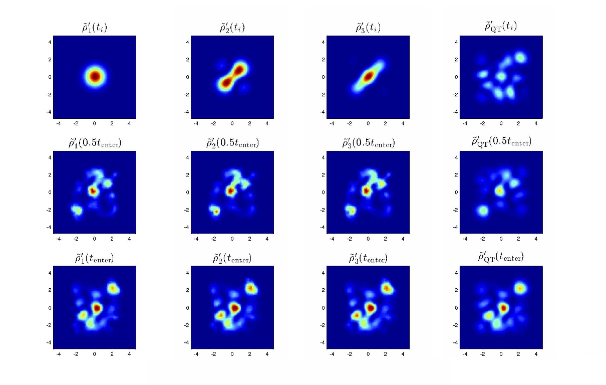
Figure 1: Relaxation in the absence of spatial expansion for different initial nonequilibria.

The results in the presence of spatial expansion are shown in Figure 2. Again, the first, second and third columns show the time evolution of the initial nonequilibrium densities (14), (15) and (16) respectively while the fourth column shows the time evolution of the quantum equilibrium density (for $M=25$). As is plain from the plots, at super-Hubble wavelengths on expanding space we find a comparable retardation or suppression of relaxation in all three cases.

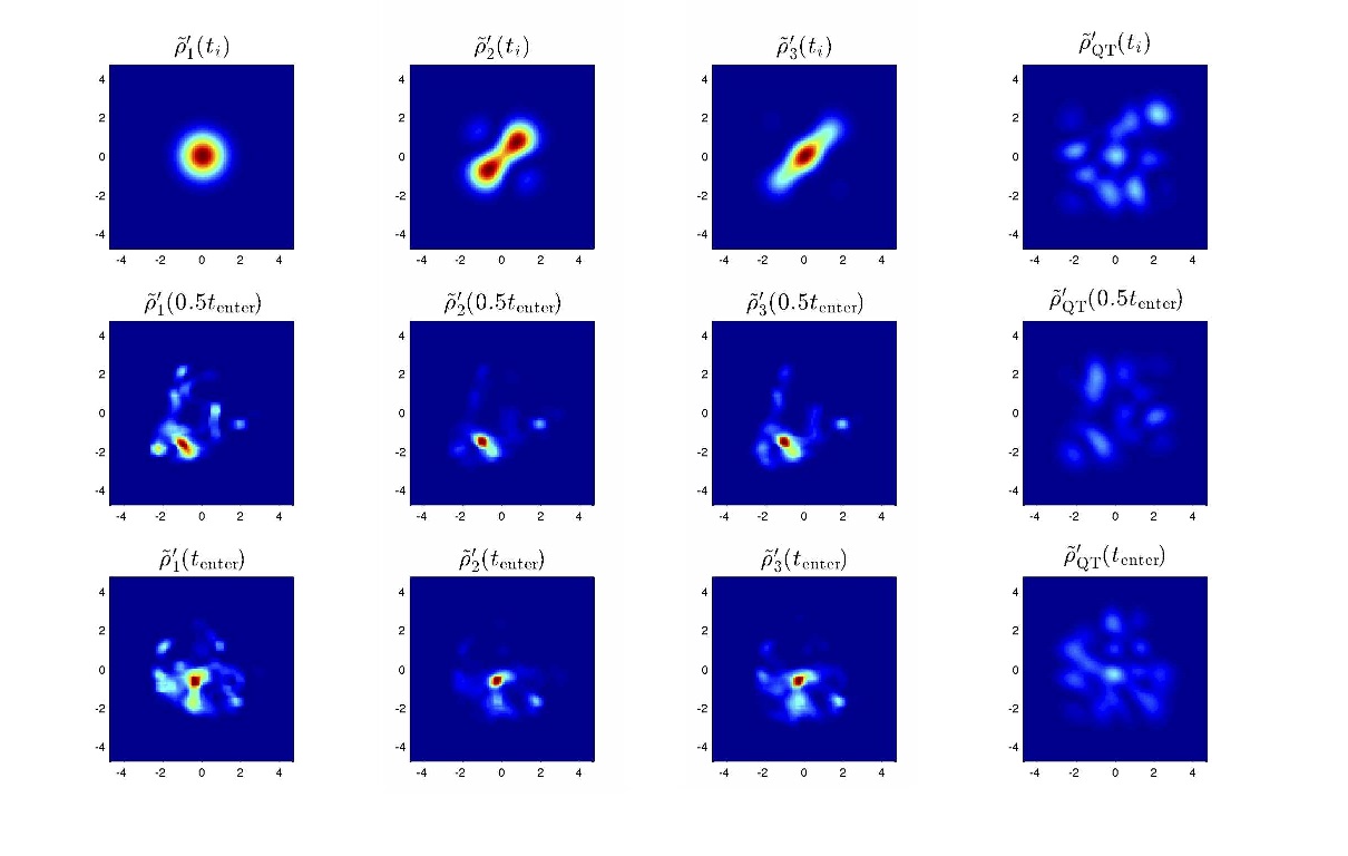
Figure 2: Relaxation suppression at super-Hubble wavelengths on expanding space for different initial nonequilibria.

3.2 Robustness of the inverse-tangent deficit $\xi(k)$

In ref. [8] we studied the deficit function $\xi(k)$ for varying numbers $M$ of modes, evolved over a fixed time interval $[t_{i},t_{f}]=[10^{-4},10^{-2}]$ and with the fixed initial nonequilibrium density (14). We found a good fit to the inverse-tangent function (13) – with small ($\lesssim 10\%$) oscillations around the curve – in all the cases $M=4,6,9,12,16,25$ that were studied. Here we consider varying the initial nonequilibrium density with fixed $M$ and evolving over the same fixed time interval $[10^{-4},10^{-2}]$. We choose the intermediate value $M=9$.

The simulation is carried out as described in detail in ref. [8]. In particular, we plot mixed-ensemble curves $\xi=\xi(k)$ obtained by averaging the variances of the densities over six sets of randomly-chosen phases in the initial wave function (9). However, in contrast to ref. [8], here we consider three different initial nonequilibrium distributions.

As shown in Figure 3, we find good fits to the inverse-tangent function (13) for all three of the initial densities (14)–(16) studied.

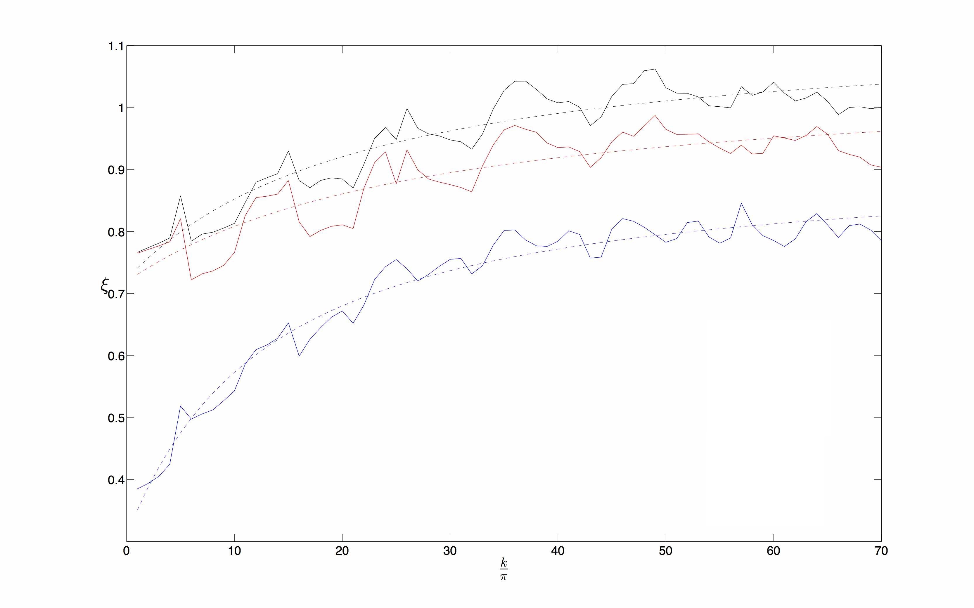
Figure 3: Mixed-ensemble curves $\xi(k)$ for the three initial nonequilibrium densities (14)–(16) ($\rho_{1}$ in blue, $\rho_{2}$ in red and $\rho_{3}$ in black), with best fits to the inverse-tangent function (13).

As shown in Table 1, the fitting coefficients $c_{1}$, $c_{2}$, $c_{3}$ depend on the initial density. The first coefficient $c_{1}$ is almost the same for the three initial densities but $c_{2}$ and $c_{3}$ vary considerably. Note that for $\rho_{2}$ and $\rho_{3}$ we find $c_{3}>1$.

$\rho$	$c_{1}$	$c_{2}$	$c_{3}$
$\rho_{1}$	0.14	1.44	0.92
$\rho_{2}$	0.11	2.86	1.06
$\rho_{3}$	0.12	2.30	1.13

Table 1: Fitting coefficients $c_{1}$, $c_{2}$, $c_{3}$ for the initial nonequilibrium densities $\rho_{1}$, $\rho_{2}$, $\rho_{3}$.

4 Radiation-dominated phase with a subsequent inflationary phase

We now consider how the deficit function $\xi(k)$ will be affected by a period of exponential (inflationary) expansion added to the end of a radiation-dominated phase. We assume the fixed initial nonequilibrium density (14) (with initial wavefunctions of the form (9)) at time $t_{i}$ at the beginning of the radiation-dominated period, which as before lasts until a time $t_{f}$; we then add an inflationary period beginning at $t_{f}$ and lasting until a time $t_{f}^{\prime}$. We shall calculate $\xi(k)$ for varying numbers $M$ of superposed energy states in the initial wavefunction.

To proceed, we must first find the retarded time function $t_{\mathrm{ret}}=t_{\mathrm{ret}}(t,k)$ for an exponential expansion. We may then add appropriate retarded time intervals (corresponding to $[t_{f},t_{f}^{\prime}]$) to the evolution of the equivalent standard oscillator for modes of wavenumber $k$, thereby obtaining the time evolution over the combined radiation-dominated and inflationary eras. From the final densities – again simulated for a mixed ensemble with six sets of randomly-chosen initial phases – we are then able to calculate the mixed-ensemble deficit function $\xi(k)$.

4.1 Retarded time for an inflationary phase

The expression for the retarded time $t_{\mathrm{ret}}=t_{\mathrm{ret}}(t,k)$ arises [7] by finding the solution for the time evolution $\psi_{n_{r}}(q_{r},t)$ of the initial wave function $\psi_{n_{r}}(q_{r},t_{i})=\Phi_{n_{r}}(q_{r})$ under a formal one-dimensional Schrödinger equation

$$i\frac{\partial\psi_{n_{r}}(q_{r},t)}{\partial t}=\left(-\frac{1}{2m}\partial_{r}^{2}+\frac{1}{2}m\omega^{2}q_{r}^{2}\right)\psi_{n_{r}}(q_{r},t)$$ (17)

with Hamiltonian $\hat{H}_{r}(t)$ (equation (4)), where

$$m\equiv a^{3}\ ,\ \ \ \omega\equiv k/a\ .$$ (18)

The exact solution with $a\propto t^{1/2}$ was found in ref. [7]. Here we wish to find the solution with an inflating scale factor

$$a(t)=a_{f}e^{H(t-t_{f})}\ ,$$ (19)

where $t_{f}$ is the time at which the inflationary phase begins (while ending at $t_{f}^{\prime}$) and $H$ is assumed to be constant.

As we saw in ref. [7], we first need to find two solutions $f_{1}$ and $f_{2}$ of the classical equation

$$\ddot{f}+\frac{\dot{m}}{m}\dot{f}+\omega^{2}f=0~{}.$$ (20)

Then we define a function

$$g_{-}=\gamma_{1}f_{1}^{2}+\gamma_{2}f_{1}f_{2}+\gamma_{3}f_{2}^{2}~{},$$ (21)

where $\gamma_{1}$, $\gamma_{2}$, $\gamma_{3}$ are constants (denoted $c_{1}$, $c_{2}$, $c_{3}$ in ref. [7]), and two other derived functions

$$g_{0}=-\frac{m}{2}\dot{g}_{-}\ ,\ \ \ \ g_{+}=m^{2}\omega^{2}g_{-}-m\dot{g}_{0}\ .$$ (22)

These functions must satisfy the initial conditions

$$g_{-}(t_{f})=\frac{1}{m_{f}}\ ,\ \ \ \ g_{0}(t_{f})=0\ ,\ \ \ \ g_{+}(t_{f})=m_{f}\omega_{f}^{2}\ .$$ (23)

The retarded time interval $\Delta t_{\mathrm{ret}}(k)$ corresponding to the standard time interval $t_{f}^{\prime}-t_{f}$ is then given by the integral

$$\Delta t_{\mathrm{ret}}(k)=\int_{t_{f}}^{t_{f}^{\prime}}\frac{dt}{m(t)g_{-}(t)}~{}.$$ (24)

(See ref. [7] for a detailed derivation.)

For the scale factor (19) we have $\dot{m}/m=3H$ and $\omega=ke^{-H(t-t_{f})}/a_{f}$. Equation (20) then becomes

$$\ddot{f}+3H\dot{f}+\kappa^{2}e^{-2H(t-t_{f})}f=0~{},$$ (25)

where $\kappa=k/a_{f}$. We find the two solutions

$$f_{1} =\cos\left((\kappa/H)e^{-H(t-t_{f})}\right)+(\kappa/H)e^{-H(t-t_{f})}\sin\left((\kappa/H)e^{-H(t-t_{f})}\right)\ ,$$ (26)

$$f_{2} =\sin((\kappa/H)e^{-H(t-t_{f})})-(\kappa/H)e^{-H(t-t_{f})}\cos((\kappa/H)e^{-H(t-t_{f})})\ .$$ (27)

From (21) and (22), together with the initial conditions (23), we obtain the constants $\gamma_{1}$, $\gamma_{2}$, $\gamma_{3}$:

$$\gamma_{1} =\frac{1}{2k^{4}a_{f}}\left(-H^{4}a_{f}^{2}\cos(2k/Ha_{f})-2H^{3}ka_{f}\sin(2k/Ha_{f})+H^{2}(H^{2}a_{f}^{2}+2k^{2})\right)\ ,$$ (28)

$$\gamma_{2} =\frac{1}{k^{4}}\left(2H^{3}k\cos(2k/Ha_{f})-Ha_{f}\sin(2k/Ha_{f})\right)\ ,$$ (29)

$$\gamma_{3} =\frac{1}{2k^{4}a_{f}}\left(H^{4}a_{f}^{2}\cos(2k/Ha_{f})+2H^{3}ka_{f}\sin(2k/Ha_{f})+H^{2}(H^{2}a_{f}^{2}+2k^{2})\right)\ .$$ (30)

The expression (21) for $g_{-}$ is now fully determined.

For the purpose of obtaining the retarded time interval, the important function is $mg_{-}$. Evaluating it explicitly, we find

$$mg_{-} =\left(-\frac{1}{2\phi_{f}\phi^{3}}-\frac{2}{\phi^{2}}+\frac{1}{2\phi_{f}\phi}\right)\cos(2\phi-2\phi_{f})+$$

$$\left(\frac{1}{\phi^{3}}-\frac{1}{\phi_{f}\phi^{2}}-\frac{1}{\phi}\right)\sin(2\phi-2\phi_{f})+$$

$$\left(\frac{1}{2\phi_{f}\phi^{3}}+\frac{\phi_{f}}{\phi^{3}}+\frac{1}{2\phi_{f}\phi}+\frac{\phi_{f}}{\phi}\right)\ ,$$ (31)

where

$$\phi\equiv(k/Ha_{f})e^{-H(t-t_{f})}\ .$$ (32)

To evaluate the integral (24), we first change variables to $\phi$ where $d\phi=-H\phi dt$. The integrand becomes

$$-\frac{2\phi_{f}}{H}\frac{\phi^{2}}{(-1-4\phi_{f}\phi+\phi^{2})\cos(2\phi-2\phi_{f})+(2\phi_{f}-2\phi-2\phi_{f}\phi^{2})\sin(2\phi-2\phi_{f})+(1+2\phi_{f}^{2}+\phi^{2}+2\phi_{f}^{2}\phi^{2})}\ .$$ (33)

We then use $\cos 2x=\cos^{2}x-\sin^{2}x$, $\sin 2x=2\sin x\cos x$ and we introduce two new functions

$$u =-\sin(\phi-\phi_{f})+\phi\cos(\phi-\phi_{f})\ ,$$ (34)

$$v =-\frac{1}{\phi_{f}}\sin(\phi-\phi_{f})+\frac{\phi}{\phi_{f}}\cos(\phi-\phi_{f})-\phi\sin(\phi-\phi_{f})-\cos(\phi-\phi_{f})~{}.$$ (35)

The integrand can then be written as

$$-\frac{1}{\phi_{f}H}\frac{(du/d\phi)v-u(dv/d\phi)}{u^{2}+v^{2}}\ .$$ (36)

An indefinite integral with respect to $\phi$ is given by

$$-\frac{1}{\phi_{f}H}\tan^{-1}(\frac{u}{v})\ .$$ (37)

However, this is discontinuous at zeros of $v$. To proceed, the domain of integration must be divided into subdomains and each time we cross a zero of $v$ we must add $\pi a_{f}/k$ to the retarded time interval. (This requires that we find the zeros of the function $v$, which is straightforward.)

4.2 Robustness of the inverse-tangent deficit $\xi(k)$

We now consider the effect of adding an inflationary phase. We take the preceding radiation-dominated period to begin at $t_{i}=10^{-4}$ and end at $t_{f}=10^{-2}$ just as before. We then take the inflationary phase to begin at $t_{f}=10^{-2}$ and end at $t_{f}^{\prime}=t_{f}+0.05=0.06$, with an inflationary Hubble constant $H=25$. The parameters have been chosen so as to yield an interesting physical range and also to enable us to carry out the numerical simulation in a reasonable amount of computer time. The chosen values are not intended to have any particular cosmological significance.

As shown in Figure 4, for these parameters the range of physical wavelengths that we consider are mostly sub-Hubble at the beginning of inflation ($t=t_{f}$) and essentially all super-Hubble at the end of inflation ($t=t_{f}^{\prime}$). The simulation will then probe what happens when modes exit the Hubble radius during inflation – a key component of the standard inflationary scenario.

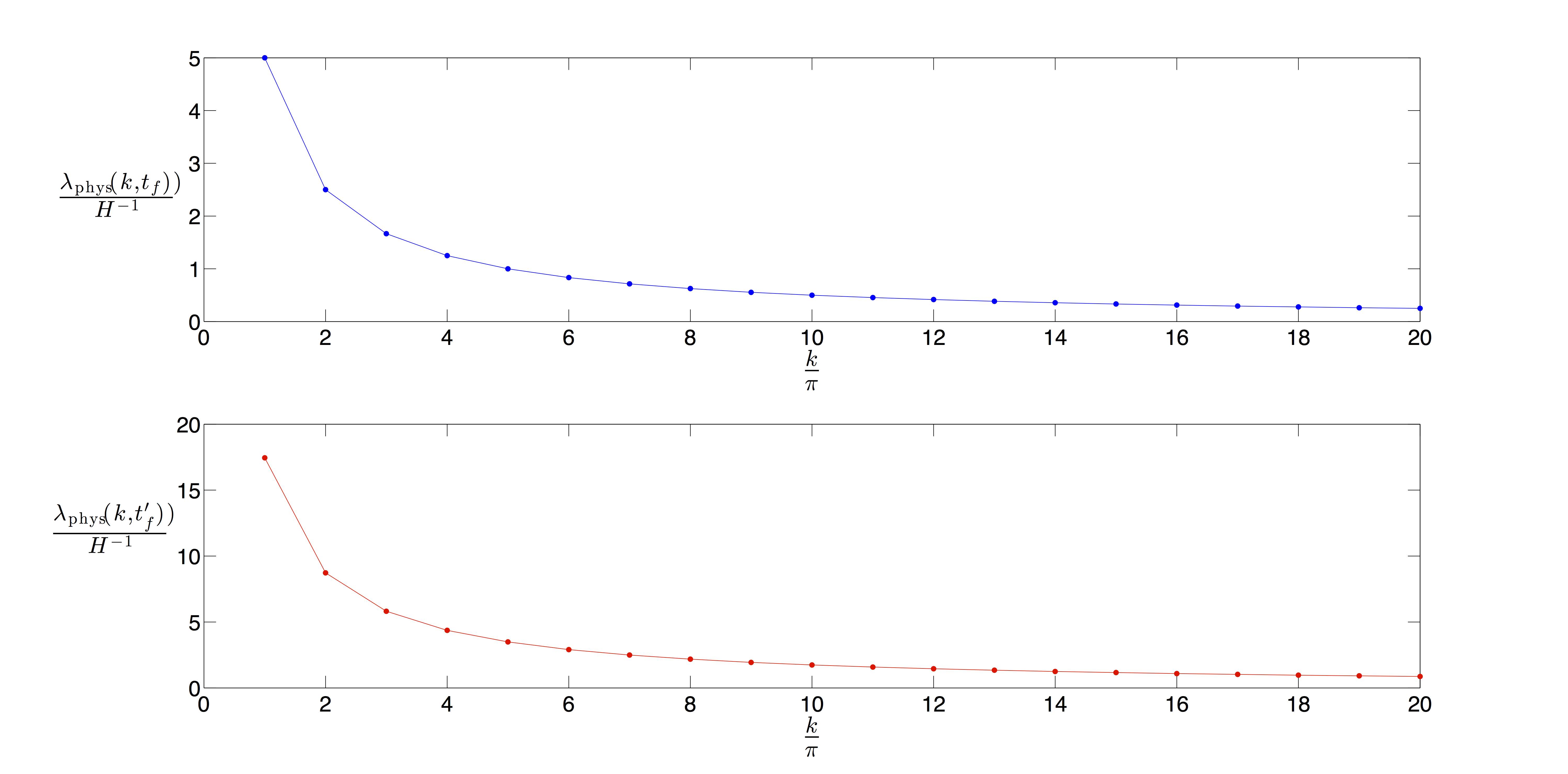
Figure 4: The top figure shows physical wavelengths as a function of $k$ at the beginning of inflation ($t=t_{f}=10^{-2}$), in units of the Hubble radius. For the range we consider, most of the modes are initially sub-Hubble. The bottom figure shows physical wavelengths as a function of $k$ at the end of inflation ($t=t_{f}^{\prime}=0.06$), again in units of the Hubble radius. For the range we consider, the final modes are essentially all super-Hubble.

Furthermore, for this set of parameters the values of the retarded time (plotted in Figure 5) are not so large as to prevent a numerical simulation in an acceptable amount of computer time. It is noteworthy that as $k$ increases the value of $\Delta t_{\mathrm{ret}}(k)$ quickly saturates.

Figure 5: Retarded time interval $\Delta t_{\mathrm{ret}}(k)$ corresponding to the lapse $t_{f}^{\prime}-t_{f}$ of standard cosmological time during the inflationary phase, plotted as a function of wavenumber $k$.

For this set of parameters, then, we numerically simulate the function $\xi(k)$ for the combined radiation and inflationary eras, taking initial wavefunctions (9) that are superpositions of $M$ energy states and with the fixed initial nonequilibrium density (14). The simulation is again carried out as described in ref. [8], plotting mixed-ensemble curves $\xi=\xi(k)$ obtained by averaging the variances over six sets of randomly-chosen initial phases, except that now the retarded time interval (for the evolution of the equivalent oscillator) is increased by the value $\Delta t_{\mathrm{ret}}(k)$ corresponding to the additional lapse $t_{f}^{\prime}-t_{f}$ of standard cosmological time during the inflationary phase. Our results for $M=4,6,9,12,16$ are shown in Figure 6. For each curve in the figure we include a fit to the inverse-tangent function (13).

Figure 6: Mixed-ensemble curves $\xi(k)$ for the combined radiation-dominated and inflationary eras, for $M=4,6,9,12,16$ modes and with the fixed initial nonequilibrium density (14), with fits to the inverse-tangent function (13).

For smaller $M$ we are able to integrate further in $k$-space since the velocity field is less erratic for smaller $M$. In Figure 6 we show all of the data that we were able to obtain to good accuracy in an acceptable amount of computer time.

Despite the limited extent of our results in $k$-space for larger $M$, the goodness of fit to the inverse-tangent function (13) is clear enough. Thus we may conclude that the inverse-tangent deficit (13) is robustly valid under the addition of an inflationary phase.

4.3 Dependence of the fitting coefficients on $M$

Given the fits to the function (13) for $M=4,6,9,12,16$, we may study how the fitting coefficients $c_{1}$, $c_{2}$, $c_{3}$ vary with $M$.

Since we have generated data for all of the considered values of $M$ only up to about $k=10\pi$, in order to compare like with like we consider it better to omit the extra data at $k>10\pi$ for the case $M=4$. Thus, for $M=4$ we truncate the curve at $k=10\pi$ before finding the fitting coefficients for the inverse-tangent function (13). With this understanding, the resulting coefficients $c_{1}$, $c_{2}$, $c_{3}$ are shown in Table 2.

$M$	$c_{1}$	$c_{2}$	$c_{3}$
$4$	$2.39$	$4.01$	$0.87$
$6$	$1.72$	$1.96$	$0.91$
$9$	$1.70$	$0.96$	$0.92$
$12$	$1.58$	$0.32$	$0.99$
$16$	$1.37$	$0.25$	$1.00$

Table 2: Fitting coefficients $c_{1}$, $c_{2}$, $c_{3}$ for varying $M=4,6,9,12,16$.

In Figure 7 we show how $c_{1}$ varies with $M$, together with a fitted curve

$$c_{1}=1.51+8.55e^{-{0.57M}}{\ .}$$ (38)

This has the same functional form (with different coefficients) as the fit found in our previous simulations for the radiation-dominated phase only [8]. While the fit is not quite as good as before, our results are consistent with the previous (approximately exponential) decay of $c_{1}$ with $M$.

Figure 7: Plot of $c_{1}$ as a function of $M$, with a best-fit curve (38).

In Figure 8 we show how $c_{2}$ varies with $M$, together with a fitted curve

$$c_{2}=0.20+16.11e^{{-0.36M}}\ .$$ (39)

Again, this has the same functional form as the fit found in our previous simulations [8] and now the goodness of fit is comparable to that found previously.

Figure 8: Plot of $c_{2}$ as a function of $M$, with a best-fit curve (39).

Finally, in Figure 9 we show how $c_{3}$ varies with $M$, together with a fitted curve

$$c_{3}=\tan^{-1}{(0.15M+2.11)}-\pi/2+1.22\ .$$ (40)

Once again this has the same functional form as the fit found previously [8] and with a fit that is not quite as good as before.

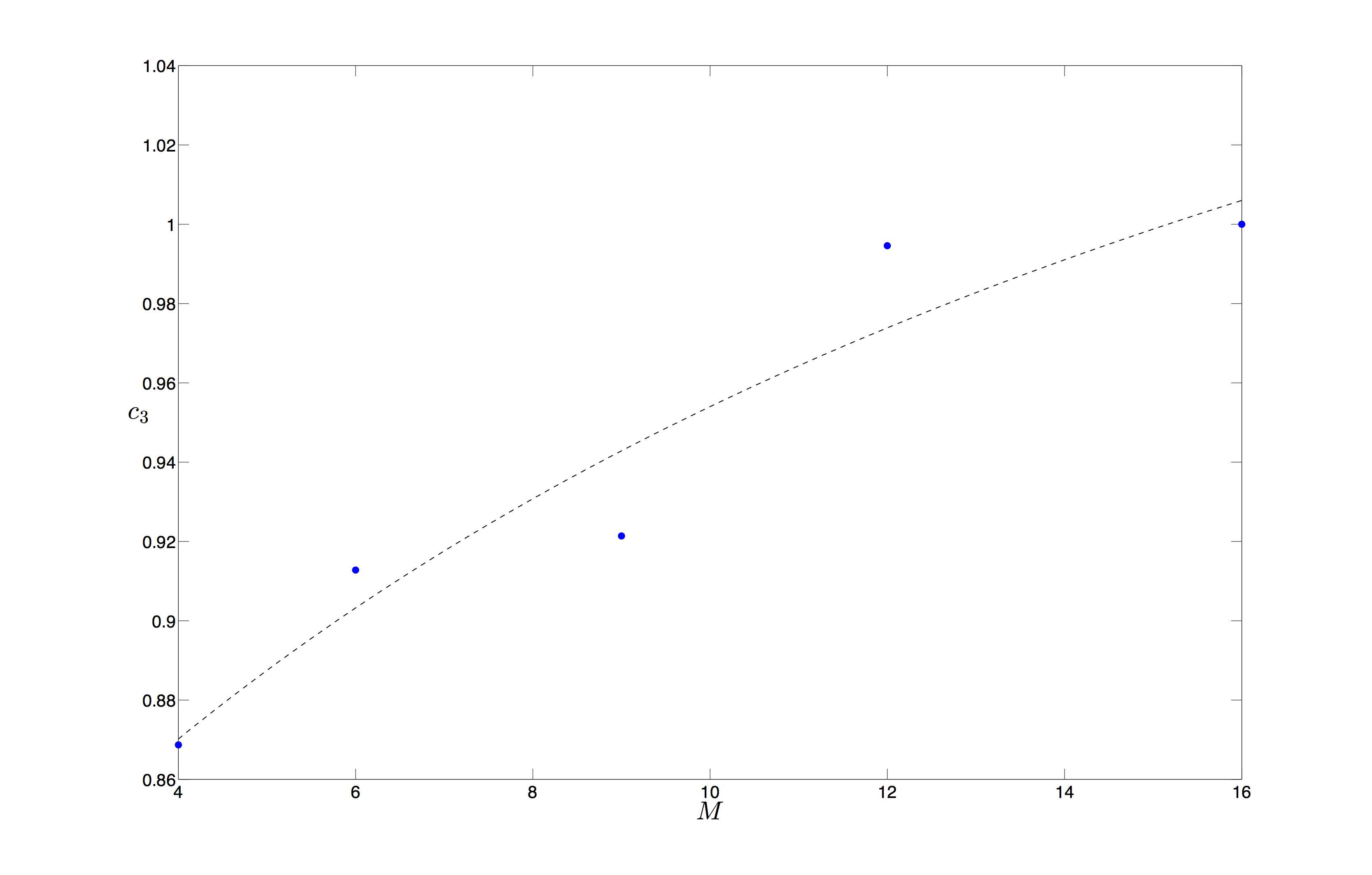
Figure 9: Plot of $c_{3}$ as a function of $M$, with a best-fit curve (40).

To a first approximation, our results for $c_{1}$, $c_{2}$, $c_{3}$ as functions of $M$ are consistent with the results found in ref. [8] for the radiation-dominated phase only. Thus, not only is the inverse-tangent fit (13) robustly valid under the addition of an inflationary phase, the functional dependence of the fitting coefficients on $M$ is also approximately maintained.

5 Conclusion

We have shown that our prediction of an inverse-tangent power deficit function $\xi(k)$ – arising from quantum relaxation on expanding space – is robust under changes in the initial nonequilibrium distribution as well as under the addition of an inflationary period to the end of the radiation-dominated phase. In both cases the simulated deficit $\xi(k)$ remains an inverse-tangent function of $k$. Furthermore, with the inflationary phase the dependence of the fitting parameters $c_{1}$, $c_{2}$, $c_{3}$ on the number $M$ of superposed pre-inflationary energy states is found to be comparable to the dependence found previously. These results suggest that, for the assumed broad class of initial conditions, the inverse-tangent function (13) is likely to be a rather general signature of quantum relaxation in the early universe. It remains to be seen how well this prediction compares with the data [29].

There is clearly a limit, however, to the robustness of our results against changes in the initial nonequilibrium distribution. As an extreme example, if a field mode had an initial delta-function distribution $\rho(q_{1},q_{2},t_{i})=\delta(q_{1}-q_{1}(t_{i}))\delta(q_{2}-q_{2}(t_{i}))$ the corresponding theoretical ensemble would contain just one trajectory beginning at $q_{1}(t_{i})$, $q_{2}(t_{i})$ and ending at $q_{1}(t_{f})$, $q_{2}(t_{f})$. The nonequilibrium distribution at later times would still be a delta-function, $\rho(q_{1},q_{2},t_{f})=\delta(q_{1}-q_{1}(t_{f}))\delta(q_{2}-q_{2}(t_{f}))$. The final variance would vanish and we would have $\xi=0$ for that mode. This could in principle happen for a range of modes or even for all modes, resulting in no primordial power at all. Clearly, for relaxation considered over a given time interval, if the initial distribution is sufficiently narrow the final function $\xi(k)$ could differ considerably from our inverse-tangent result (13). In our simulations we have taken initial states that depart fairly mildly from quantum equilibrium, and for these we have found a final inverse-tangent deficit over a range of initial conditions. In this sense our results are robust. But if the changes in the initial state are too extreme, then with a fixed time interval our inverse-tangent prediction will necessarily fail. On the other hand, if the considered time interval is not fixed, then even for very narrow initial nonequilibria one might obtain results resembling ours if only the modes are evolved over a sufficiently long cosmological time. We leave a study of this last point for future work.

Some assumptions certainly need to made about initial conditions, otherwise it is impossible to make predictions. In our simulations we have always considered initial distributions $\rho(q_{1},q_{2},t_{i})$ of width smaller than the width of $|\psi(q_{1},q_{2},t_{i})|^{2}$. This may be justified partly on heuristic grounds: if we regard quantum noise as having a dynamical origin, it is natural to assume initial conditions such that the initial state has less noise (or a smaller statistical spread) than a conventional quantum state. We also assume that $\rho(q_{1},q_{2},t_{i})$ is appropriately smooth, in the sense of not possessing any significant fine-grained microstructure – an assumption that is required to obtain relaxation in any time-reversal invariant theory [17, 18, 19, 31]. Our assumed initial conditions have been guided by simplicity and heuristic arguments. Their ultimate justification rests on how well our predictions compare with data.

We should also mention a further caveat. We have restricted ourselves to initial quantum states (at the beginning of pre-inflation) of the form (9). These are equally-weighted superpositions of energy eigenstates with randomly-chosen phases. One might ask if our results are also robust under changes to more general initial quantum states. In fact, all previous studies of relaxation have assumed such equally-weighted superpositions. We leave the study of more general superpositions for future work.

There is a remaining gap in our scenario. We do not have a proper treatment of the transition from pre-inflation to inflation. In our simulations, we regard the behaviour of the free scalar field $\phi$ as representative of the behaviour of whatever fields may have been present during pre-inflation. We have not specified the relation between $\phi$ and the inflaton field. Our simulations yield a correction $\xi(k)$ to the power spectrum of $\phi$ and we simply assume that the same correction appears in the inflationary spectrum [6, 7, 8]. Adding an inflationary period to our simulations of relaxation for $\phi$ is a step towards filling the gap in our model. However, a proper understanding requires a full field-theoretical model of the transition from pre-inflation to inflation, which may involve symmetry breaking and associated field redefinitions. We hope to develop such a model in future work, and to run the appropriate numerical simulations required to obtain the exact predicted deficit function $\xi(k)$.

Acknowledgements. We are grateful to Murray Daw for kindly providing us with extra computational resources on the Clemson University Palmetto Cluster. This research was supported in part by the John Templeton Foundation and by Clemson University.

References

- [1] A. R. Liddle and D. H. Lyth, Cosmological Inflation and Large-Scale Structure (Cambridge University Press, Cambridge, 2000).
- [2] V. Mukhanov, Physical Foundations of Cosmology (Cambridge University Press, Cambridge, 2005).
- [3] P. Peter and J.-P. Uzan, Primordial Cosmology (Oxford University Press, 2009).
- [4] A. Valentini, Astrophysical and cosmological tests of quantum theory, J. Phys. A: Math. Theor. 40, 3285 (2007). [arXiv:hep-th/0610032]
- [5] A. Valentini, De Broglie-Bohm prediction of quantum violations for cosmological super-Hubble modes, arXiv:0804.4656 [hep-th].
- [6] A. Valentini, Inflationary cosmology as a probe of primordial quantum mechanics, Phys. Rev. D 82, 063513 (2010). [arXiv:0805.0163]
- [7] S. Colin and A. Valentini, Mechanism for the suppression of quantum noise at large scales on expanding space, Phys. Rev. D 88, 103515 (2013). [arXiv:1306.1579]
- [8] S. Colin and A. Valentini, Primordial quantum nonequilibrium and large-scale cosmic anomalies, Phys. Rev. D 92, 043520 (2015). [arXiv:1407.8262]
- [9] A. Valentini, Statistical anisotropy and cosmological quantum relaxation, arXiv:1510.02523.
- [10] L. de Broglie, La nouvelle dynamique des quanta, in: Électrons et Photons: Rapports et Discussions du Cinquième Conseil de Physique (Gauthier-Villars, Paris, 1928). [English translation in ref. [11].]
- [11] G. Bacciagaluppi and A. Valentini, Quantum Theory at the Crossroads: Reconsidering the 1927 Solvay Conference (Cambridge University Press, 2009). [arXiv:quant-ph/0609184]
- [12] D. Bohm, A suggested interpretation of the quantum theory in terms of ‘hidden’ variables. I, Phys. Rev. 85, 166 (1952).
- [13] D. Bohm, A suggested interpretation of the quantum theory in terms of ‘hidden’ variables. II, Phys. Rev. 85, 180 (1952).
- [14] P. R. Holland, The Quantum Theory of Motion: an Account of the de Broglie-Bohm Causal Interpretation of Quantum Mechanics (Cambridge University Press, Cambridge, 1993).
- [15] A. Valentini, Signal-locality, uncertainty, and the subquantum H-theorem. I, Phys. Lett. A 156, 5 (1991).
- [16] A. Valentini, Signal-locality, uncertainty, and the subquantum H-theorem. II, Phys. Lett. A 158, 1 (1991).
- [17] A. Valentini, On the pilot-wave theory of classical, quantum and subquantum physics, PhD thesis, International School for Advanced Studies, Trieste, Italy (1992). [http://urania.sissa.it/xmlui/handle/1963/5424]
- [18] A. Valentini, Pilot-wave theory of fields, gravitation and cosmology, in: Bohmian Mechanics and Quantum Theory: an Appraisal, eds. J. T. Cushing et al. (Kluwer, Dordrecht, 1996).
- [19] A. Valentini, Hidden variables, statistical mechanics and the early universe, in: Chance in Physics: Foundations and Perspectives, eds. J. Bricmont et al. (Springer, Berlin, 2001). [arXiv:quant-ph/0104067]
- [20] A. Valentini, Subquantum information and computation, Pramana – J. Phys. 59, 269 (2002). [arXiv:quant-ph/0203049]
- [21] A. Valentini, Beyond the quantum, Physics World 22N11, 32 (2009). [arXiv:1001.2758]
- [22] A. Valentini, De Broglie-Bohm pilot-wave theory: Many-worlds in denial?, in: Many Worlds? Everett, Quantum Theory, and Reality, eds. S. Saunders et al. (Oxford University Press, 2010). [arXiv:0811.0810]
- [23] P. Pearle and A. Valentini, Quantum mechanics: generalizations, in: Encyclopaedia of Mathematical Physics, eds. J.-P. Françoise et al. (Elsevier, North-Holland, 2006). [arXiv:quant-ph/0506115]
- [24] B. A. Powell and W. H. Kinney, Pre-inflationary vacuum in the cosmic microwave background, Phys. Rev. D 76, 063512 (2007).
- [25] I.-C. Wang and K.-W. Ng, Effects of a preinflation radiation-dominated epoch to CMB anisotropy, Phys. Rev. D 77, 083501 (2008).
- [26] P. A. R. Ade et al. (Planck Collaboration), Planck 2013 results. XV. CMB power spectra and likelihood, Astron. Astrophys. 571, A15 (2014). [arXiv:1303.5075]
- [27] N. Aghanim et al. (Planck Collaboration), Planck 2015 results. XI. CMB power spectra, likelihoods, and robustness of parameters, arXiv:1507.02704.
- [28] C. J. Copi, D. Huterer, D. J. Schwarz and G. D. Starkman, Lack of large-angle TT correlations persists in WMAP and Planck, Mon. Not. Roy. Astron. Soc. 451, 2978 (2015). [arXiv:1310.3831]
- [29] P. Peter, A. Valentini, S. D. P. Vitenti, in preparation.
- [30] W. Struyve and A. Valentini, De Broglie-Bohm guidance equations for arbitrary Hamiltonians, J. Phys. A: Math. Theor. 42, 035301 (2009). [arXiv:0808.0290]
- [31] A. Valentini and H. Westman, Dynamical origin of quantum probabilities, Proc. Roy. Soc. Lond. A 461, 253 (2005). [arXiv:quant-ph/0403034]
- [32] C. Efthymiopoulos and G. Contopoulos, Chaos in Bohmian quantum mechanics, J. Phys. A: Math. Gen. 39, 1819 (2006).
- [33] M. D. Towler, N. J. Russell, and A. Valentini, Time scales for dynamical relaxation to the Born rule, Proc. Roy. Soc. Lond. A 468, 990 (2012). [arXiv:1103.1589]
- [34] S. Colin, Relaxation to quantum equilibrium for Dirac fermions in the de Broglie–Bohm pilot-wave theory, Proc. Roy. Soc. Lond. A 468, 1116 (2012). [arXiv:1108.5496]
- [35] E. Abraham, S. Colin and A. Valentini, Long-time relaxation in pilot-wave theory, J. Phys. A: Math. Theor. 47, 395306 (2014). [arXiv:1310.1899]