The intrinsic value of HFO features as a
biomarker of epileptic activity.

Abstract

High frequency oscillations (HFOs) are a promising biomarker of epileptic brain tissue and activity. HFOs additionally serve as a prototypical example of challenges in the analysis of discrete events in high-temporal resolution, intracranial EEG data. Two primary challenges are 1) dimensionality reduction, and 2) assessing feasibility of classification. Dimensionality reduction assumes that the data lie on a manifold with dimension less than that of the features space. However, previous HFO analysis have assumed a linear manifold, global across time, space (i.e. recording electrode/channel), and individual patients. Instead, we assess both a) whether linear methods are appropriate and b) the consistency of the manifold across time, space, and patients. We also estimate bounds on the Bayes classification error to quantify the distinction between two classes of HFOs (those occurring during seizures and those occurring due to other processes). This analysis provides the foundation for future clinical use of HFO features and guides the analysis for other discrete events, such as individual action potentials or multi-unit activity.

Index Terms—  high-frequency oscillation, intrinsic dimension, dimensionality reduction, classification error, divergence

1 Introduction

About one third of epilepsy patients fail to obtain seizure control with available pharmaceuticals. One of the few options for these refractory patients is resective surgery—removing the portion of the brain thought to be causing the seizures. This region is denoted the seizure onset zone (SOZ). In some cases, determining the SOZ involves a highly invasive surgery to place electrodes on the brain’s surface, followed by one to two weeks of recording and monitoring. A second invasive surgery is performed if the SOZ can be identified and safely resected. A schematic relating the implanted electrodes with the recorded data is shown in Fig 1.

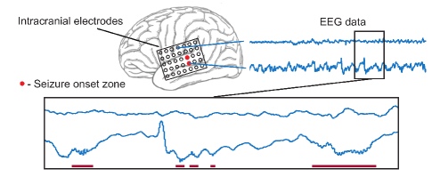
Fig. 1: Diagram relating the recorded data with the implanted electrodes. A $5\times 7$ grid of electrodes placed over a region of cortex. Each channel produces a separate time series of data, with some channels being identified by clinicians as seizure onset zone (SOZ). HFO detections are marked by solid magenta lines under the EEG trace.

A proposed biomarker to improve the localization of the SOZ are high frequency oscillations (HFOs) [1, 2]. HFOs are high frequency (about 80–300 Hz), short ($<50$ ms), rare events occurring in intracranial EEG recorded at sampling rates of several kHz. Example HFO detections and a recorded seizure are shown in Fig 2.

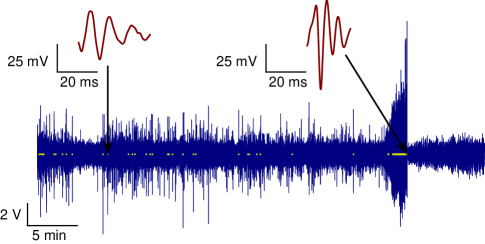
Fig. 2: Example HFO detections within 45 min of one channel of intracranial EEG data. A seizure occurs at about 35 minutes. HFO detections (72 interictal and preictal, 32 ictal) are shown as small yellow dots. Two HFOs are also shown using a much smaller scale.

Much of the published research on HFOs uses human identified HFOs in short (10 to 20 minute) recordings [3, 4]. These results have shown that a high HFO occurrence rate is correlated with the SOZ. However, recent work is moving towards automated identification and analysis of HFOs in long term, high resolution data, which requires advanced computational and statistical techniques [5]. Quality recordings may span 7-14 days, with over 100,000 HFO detections in several terabytes of data. Thus, the next advances are expected to come through big data analysis of HFO features, utilizing millions of recorded HFOs across as many patients as possible [6].

Relatively few research groups have analyzed HFO features in detail. The most advanced analysis computed six features of about 300,000 HFOs in nine patients and two controls, and utilized a global PCA across all channels followed by $k$-means clustering [7, 8, 9]. The authors implicitly assumed that the distribution of these HFO features lies on a linear manifold in feature space, and that the manifold is consistent across time and space (i.e., recording electrode).

The other most advanced analysis compared HFOs produced in the motor cortex via movement versus HFOs occurring in the SOZ, utilizing three features and a support vector machine (SVM) classifier [10]. Some differences were noted, but a more general analysis that addresses the degree to which HFOs produced by pathological activity or networks (denoted pathological HFOs or pHFOs) and HFOs produced by normal, physiological activity (denoted normal HFOs or nHFOs) are observably different has not been performed.

The goals of this work are to test the implicit assumptions previously used in HFO feature analysis. Specifically, the goals are to 1) assess the type of manifold on which HFO features lie, and 2) assess how discernible pHFOs are from nHFOs, based on their feature-space distributions.

The general outline is as follows. To assess the linearity of the HFO-feature manifold, a non-linear, local estimate of intrinsic dimension [11, 12] is compared with a linear global estimate (PCA) applied to local subsets. This approach is similar to that in [13]. The corresponding reduced dimension subspaces are individually compared across time and space using a modified Grassmann distance, building off the work in [14]. We additionally use a greedy Fisher LDA algorithm (similar to the greedy LDA in [15]) to identify a basis that maximally separates pHFOs from nHFOs. Unsupervised clustering of the subspaces is then compared with channel groups based on clinical markings of the SOZ and physical groupings of the electrodes. Lastly, we assess the discernibility of nHFOs and pHFOs by estimating bounds on the Bayes Error using the Henze-Penrose divergence (HPD) [16, 17].

2 Patient population and data

EEG data from adult patients with refractory epilepsy who underwent intracranial EEG monitoring were selected from the IEEG Portal [18] and from the University of Michigan. All patient data was included which met the following criteria: sampling rate of at least 5 kHz, recording time greater than one hour, data recorded with traditional intracranial electrodes, and available meta-data regarding seizure times and the resected volume or SOZ. This yielded 17 patients, (nine IEEG portal, eight U. of M.). All data were acquired with approval of local institutional review boards (IRB), and all patients consented to share their de-identified data. Of these 17 patients, 13 had recorded seizures, nine were known to have resection and obtained seizure-freedom (ILAE class I), with eight patients in common between these two categories. Because these surgeries are relatively rare, this patient population size is moderately large for analysis of intracranial EEG data.

HFOs were detected using the qHFO algorithm [5], resulting in over 1.6 million HFOs in nearly 100,000 channel-hours of 5 kHz data. Each HFO was band pass filtered between 80 to 500 Hz using an elliptical filter and 33 features were computed, including duration, peak power, mean of the Teager-Kaiser energy [19], and various spectral properties. Ictal is defined as during seizures, with seizures assumed to be five minutes long if the length was not specified in available meta-data. Interictal is defined as at least 30 minutes from the start or end of a seizure, based on [9].

3 Dimensionality reduction

3.1 Consistency of local, non-linear intrinsic dimension

To assess both the linearity and local versus global nature of the HFO feature manifold, the non-linear intrinsic dimension was computed via the $k$-nearest neighbor (NN) based estimator in [11]. This estimator estimates the intrinsic dimension by exploiting its relationship to the total edge length of the $k$-NN graph. This nonlinear estimator provides a local estimate of intrinsic dimension which enables us to identify local variations in data manifolds. The result is an estimate of the intrinsic dimension for each given HFO, which are then averaged to obtain the mean intrinsic dimension for a given partition of the data. The consistency of the manifold is measured by comparing the distribution of intrinsic dimension across time, space and patients. The specific comparisons are: a) interictal versus ictal times, per channel, b) time variation within interictal periods, per channel, and c) comparisons between channels, integrated over time.

A variety of methods could be employed to compare the intrinsic dimension for two disjoint sets of HFOs. However, the final dimension selected will be an integer. Thus, small differences in the intrinsic dimension between two sets, no matter how statistically significant, are not meaningfully different if they mean value for each set round to the same integer.

To compare two sets of intrinsic dimension, we define a distance measure, $\theta_{I}$, between collections of integers. Let the two sets of integers be $A$ and $B$, and let $n_{i}$ be the fraction of elements in $A$ equal to $i$, and $m_{i}$ be the fraction of elements in $B$ equal to $i$. The probability that two elements in set $A$ are equal is $\bm{n}^{T}\bm{n}$, and the probability that an element of $A$ is equal to an element of $B$ is $\bm{n}^{T}\bm{m}$. A measure of distance between $A$ and $B$ is how likely an element of $A$ is equal to an element of $B$, normalized by the likelihoods of elements being equal another element in the same group:

$$\theta_{I}=\arccos\left(\frac{\bm{n}^{T}\bm{m}}{\sqrt{\bm{n}^{T}\bm{n}}\sqrt{\bm{m}^{T}\bm{m}}}\right),$$ (1)

The value $\theta_{I}$ is the angle between $\bm{n}$ and $\bm{m}$ and provides an easy interpretation as to the consistency of two different collections of local intrinsic dimensional. This quantity is also know as the angular distance or angular dissimilarity, and is the inverse cosine of the Ochiai-Barkman coefficient [20, 21].

We compute the $\theta_{I}$-distance for three different comparisons of HFOs: 1) a comparison of each pair of 30 minute time windows on a given channel for a given patient, 2) a comparison of ictal versus interictal periods, again on a given channel for a given patient, and 3) a comparison of different channels in a given patient during interictal periods. Interictal-ictal comparisons where one set of events is less than 50 HFOs are ignored. Histograms of the distribution of $\theta_{I}$ for each type of comparison are shown in Fig. 3. This figure involves over 5 million interictal time bin comparisons, 163 ictal versus interictal comparisons, over 36 thousand interictal channel-channel comparisons and almost 10 thousand ictal channel-channel comparisons.

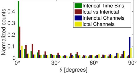
Fig. 3: Comparisons of the consistency of the intrinsic dimension ($\theta_{I}$ from Eq. 1) for four comparisons, as described in the text. Note, $0^{\circ}$ implies no difference and $90^{\circ}$ implies maximal difference between the two collections of intrinsic dimension being compared.

The intrinsic dimension is quite consistent across different time segments during interictal times (strong peak near $0^{\circ}$), but has some variance between ictal and interictal times (still peaked near $0^{\circ}$ but the peak is wider). The dimension is less consistent across channels, with comparisons during ictal times showing small peaks at both $0^{\circ}$ and $90^{\circ}$, and interictal having the largest peak at $90^{\circ}$, showing maximal difference. Thus we see that the intrinsic dimension varies significantly across channels, especially for interictal HFOs.

3.2 Comparison with Global Linear Intrinsic Dimension

Next we compare the $k$-NN intrinsic dimension estimate of Section 3.1 with a global, linear method to assess how linear and/or local the feature manifold is. The most common global, linear method of intrinsic dimension estimation and dimensionality reduction is principle component analysis (PCA), which we perform by first centering the data and then using singular value decomposition (SVD). PCA is performed multiple times for the same divisions of the HFO data as done for Fig. 3. Subsets of HFOs with less than 50 events are ignored, as these are deemed insufficient to estimate the PCA vectors in 33D. This results in PCA vectors being computed for 606 of the 1318 channels (12 patients) for interictal HFOs, 171 channels for ictal HFOs (8 patients), and 163 channels comparing ictal versus interictal (8 patients). In patients that had multiple recording sessions, channels are counted once per each session.

To compare the $k$-NN (non-linear) and PCA intrinsic dimension per channel, we 1) select the number of principle components equal to the non-linear intrinsic dimension estimate, and then 2) report the fraction of the variance accounted for by that number of principle components. This is repeated for all 606 channels (interictal) and 171 channels (ictal). When using either ictal or interictal HFOs, the median fraction of variance was 99.8%, with 99%-tile of the channels being above 89.5% (interictal) and 97.1% (ictal). It is likely that that noise in the data could account for up to 10% of the variance, and thus we conclude that the feature manifolds are approximately linear over the locality of a given channel and ictal state.

3.3 Comparison between Local Manifolds

In addition to the earlier comparison of the subspace dimensionality across channels, the next step is to directly compare the subspaces selected by the dimensionality reduction. We use a generalization of distance in the Grassmann space, which allows comparison of affine subspaces with unequal dimension [14]. The method augments the principle angles (defined in [22]) with enough additional angles (all equal to $\pi/2$) to increase the number of angles to the dimensionality of the larger space. An additional “direction vector” is also added to account for the affine offset.

We apply this generalization [14] to a new modification of the chordal distance, defined as

$$\theta_{C}=\arcsin\left(\left(\frac{1}{k}\sum_{i=1}^{k}\sin^{2}\theta_{i}\right)^{1/2}\right),$$ (2)

for $k$ principle angles $\{\theta_{i}\}_{i=1}^{k}$. The two modifications are 1) dividing by $k$, which allows the distance to be independent on the dimensionality of the spaces being compared, and 2) converting the distance measure back to an angle, which is more intuitive.

We then compare the subspaces obtained by PCA dimensionality reduction, for the same divisions of the data as used for Fig. 3. However, we now ignore any subsets of less than 50 HFOs, as these are deemed unreliable for computing the PCA in 33D. Note this figure still involves over 200 thousand time bin comparisons, the same 163 ictal versus interictal comparisons, and nearly 3,500 of each type of channel-channel comparisons.

Results for these comparisons are shown in Fig. 4. We observe that the PCA subspaces are quite consistent across different time bins, with the distributions for PCA subspaces all peaking less than $15^{\circ}$ and not extending much past $20^{\circ}$.

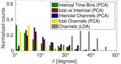
Fig. 4: Comparison of the subspaces from the PCA and greedy Fisher LDA dimensionality reduction, using $\theta_{C}$ (Eq. 2), for the same types of comparisons as Fig. 3. Again, $0^{\circ}$ implies maximally similar and $90^{\circ}$ implies maximally different.

4 Pathological versus Normal HFOs

4.1 Dimensionality Reduction: Greedy Fisher LDA

While the subspaces obtained via PCA represent the variance well, they are not necessarily the optimal directions for separating the feature distributions of pHFOs and nHFOs. An alternate dimensionality reduction method is used: greedy Fisher’s LDA. In this method, Fisher’s LDA is applied, resulting in a single basis direction. The projection of the data in this direction is then subtracted from the data, and the process is repeated.

Recall that Fisher’s LDA uses the sum of the covariance of each group, rather than the covariance of the pooled groups [23]. Letting the mean and covariance of the two groups be denoted $\mu_{A}$, $\mu_{B}$ and $\Sigma_{A}$, $\Sigma_{B}$, respectively, the specific direction is given by

$$w\propto\left(\Sigma_{A}+\Sigma_{B}\right)^{-1}\left(\bm{\mu}_{A}-\bm{\mu}_{B}\right).$$ (3)

Note, the rank of the sum of the covariances will be reduced by one in each step. Thus, to invert the matrix, the eigenvalue method is used, with the inverse of the eigenvalues corresponding to the removed projections being set to zero.

We compute this basis, comparing ictal versus interictal times, for the 13 patients with recorded seizures. We select the number of basis vectors equal to the mean intrinsic dimension. We again compare the basis vectors using Eq. 2, with the results shown in Fig. 4. The LDA subspaces vary much more across channels than the PCA subspaces, with the $\theta_{C}$ distribution for LDA being almost fully localized between $30^{\circ}$ and $50^{\circ}$. Note that $45^{\circ}$ implies that the subspaces overlap by half. Thus, the Fisher LDA subspaces show that some differences in ictal versus interictal HFO features are consistent between channels, while other differences are not conserved.

4.2 Bayes Error Estimates of pHFOs versus nHFOs

Next we quantify how distinct the feature distributions of pHFOs and nHFOs are, per channel. This quantification serves as a guide for future work. We utilize the Henze-Penrose divergence (HPD) [16, 17] to compute bounds on the Bayes Error. Note that small upper bounds imply highly separable classes, whereas upper bounds near 0.5 imply inseparable classes. We estimate the HPD bound using the nonparametric ensemble estimator derived in [24, 25], which achieves the parametric convergence rate.

The left panel of Fig. 5 shows the Bayes Error bound estimates for the 163 channels (eight patients) with at least 50 HFOs in each of the ictal and interictal states. Channels are separated between SOZ (27 channels) and non-SOZ (124 channels) for patients with ILEA Class I (the best) surgery outcome, and an “other” category (12 channels), including channels from patients with either worse surgery outcomes, no surgery, or missing meta-data.

Patients with Both SOZ and non-SOZ channels in ILAE class I patients (best surgery outcome) have the Bayes Error rate bound to relatively small values. However, channels in other patients have a more diffuse distribution of upper bounds, with the most probable upper bound about 0.25. It is expected that ictal HFOs are almost entirely pHFOs (on any channel), that interictal HFOs on non-SOZ channels are predominately nHFOs, and that interictal HFOs on SOZ channels are a mixture of both pHFOs and nHFOs. Thus, it is expected that the Bayes Error bounds would be lower for non-SOZ channels. Overall, these bounds suggest that there is sufficient separation between pHFO and nHFO feature distributions to allow classification of pHFOs and nHFOs in most channels.

The right panel of Fig. 5 displays the lower bound versus a linear error estimate. The linear estimate was computed with 10-fold cross validation in the Fisher LDA space by using a “box” classification boundary, with the threshold in each dimension being the value for which the receiver operator curve has largest transverse distance from the diagonal. Linear regression was also performed, resulting in an offset of 0.06 (0.04–0.08 at 95% C.L.) and a slope of 1.05 (0.82–1.28 at 95% C.L.). Thus, in aggregate this “box” classifier is already relatively close to the bound on the Bayes Error, though many individual channels are still quite far from the bound.

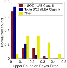
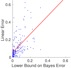
Fig. 5: Distribution of upper Bayes Error bound based on Henze-Penrose divergences (HPD) between ictal and interictal HFOs per channel. Left panel: upper bounds stratified by channel type. Bounds near zero imply high distinction between pHFOs and nHFOs, and bounds near 0.5 imply no distinction. Right panel: comparison between lower bound estimate and a linear error estimate (see the text), including the linear regression fit.

5 Clustering Channels based on subspaces

Given the observed variations in greedy Fisher LDA subspaces across channels, we seek to compare the natural clustering of these subspaces with known groupings of channels. The most relevant groupings of channels are the groups based on the physical configuration of the recording electrodes (several grids or strips of electrodes are implanted for each patient), as well as the clinically determined SOZ and resected volume for ILAE Class I patients.

The unsupervised clustering is obtained by first converting the matrix of modified chordal distances (Eq. 2) between channels per each patient to a metric using the method of dual-rooted-trees followed by spectral clustering [26]. This method adapts to the natural geometry of the data and is competitive with other algorithms [26]. We select either two groups (as the SOZ and resected volume clustering is binary) or the number of groups equal to the number of strips and grids. The unsupervised clustering results are compared with these labels using the adjusted Rand index (ARI) [27]. Unfortunately, the requirement that there be at least 50 ictal HFOs reduces the number of channels per patient significantly, resulting in only a few (4–5) patients having enough channels to cluster. However, the ARI never exceeded 0.02 for any of these comparisons in any patients, suggesting that the primary distinction between channels is not the pathology or the grid/strip placing, but other effects.

6 Discussion and Conclusion

Overall, we observe that the HFO features tend to cluster on linear manifolds. Both the subspaces of these manifolds and the local intrinsic dimension tend to be consistent within interictal periods, but may change between interictal and ictal periods. We especially note significant differences in both the intrinsic dimension and feature manifolds between different channels within the same patient. Thus, dimensionality reduction and feature analysis must account for variations between channels. The dominant cause of this inter-channel variation does not appear to be tissue pathology or grid/strip groups in the recording. We also observe that pHFOs and nHFOs are indeed distinct on a large number of channels, suggesting a strong potential for classifying individual HFOs.

This analysis also demonstrates methods applicable to other discrete events, including using the $\theta_{I}$ statistic for comparing local, intrinsic dimension for collections of events, an affine Grassmann distance $\theta_{C}$ for comparing consistency of subspaces, and estimating bounds on the Bayes Error to assess the feasibility of low-error classification. Future work will extend this analysis to a larger patient population, and classify HFOs and/or recording channels based on HFO features.

References

- [1] SC Park, SK Lee, H Che, and Chung CK, “Ictal high-gamma oscillation (60-99 hz) in intracranial electroencephalography and postoperative seizure outcome in neocortical epilepsy,” Clin. Neurophysiol., vol. 123, no. 6, pp. 1100–10, 2012.
- [2] JR Cho, DL Koo, EY Joo, DW Seo, SC Hong, P Jiruska, and SB Hong, “Resection of individually identified high-rate high-frequency oscillations region is associated with favorable outcome in neocortical epilepsy,” Epilepsia, vol. 55, pp. 1872–83, 2014.
- [3] C Haegelen, P Perucca, CE Châtillon, L Andrade-Valença, R Zelmann, J Jacobs, DL Collins, F Dubeau, A Olivier, and J Gotman, “High‐frequency oscillations, extent of surgical resection, and surgical outcome in drug‐resistant focal epilepsy,” Epilepsia, vol. 54, pp. 848–57, 2013.
- [4] K Kerber, M Dümpelmann, B Schelter, P Le Van, R Korinthenberg, A Schulze-Bonhage, and J Jacobs, “Differentiation of specific ripple patterns helps to identify epileptogenic areas for surgical procedures,” Clin. Neurophysiol., vol. 125, pp. 1339–1345, 2014.
- [5] S Gliske, Z Irwin, C Chestek, and WC Stacey, “Automated identification of seizure onset zone with a universal detector of high frequency oscillations,” Clin. Neurophysiol., vol. INSERT, 2015.
- [6] GA Worrell, K Jerbi, K Kobayashi, JM Lina, R Zelmann, and M Le Van Quyen, “Recording and analysis techniques for high-frequency oscillations,” Prog. Neurobiol., vol. 98, pp. 265–278, 2012.
- [7] JA Blanco, M Stead, A Krieger, J Viventi, WR Marsh, KH Lee, GA Worrell, and B Litt, “Unsupervised classification of high-frequency oscillations in human neocortical epilepsy and control patients,” J Neurophysiol, vol. 104, pp. 2900–2912, 2010.
- [8] JA Blanco, M Stead, A Krieger, W Stacey, D Maus, E Marsh, J Viventi, KH Lee, R Marsh, B Litt, and GA Worrell, “Data mining neocortical high-frequency oscillations in epilepsy and controls,” Brain, vol. 134, pp. 2948–2959, 2011.
- [9] A Pearce, D Wulsin, JA Blanco, A Krieger, B Litt, and WC Stacey, “Temporal changes of neocortical high-frequency oscillations in epilepsy,” J. Neurophysiol, vol. 110, pp. 1167–1179, 2013.
- [10] A Matsumoto, BH Brinkmann, SM Stead, J Matsumoto, MT Kucewicz, WR Marsh, F Meyer, and G Worrell, “Pathological and physiological high-frequency oscillations in focal human epilepsy,” J. Neurophysiol., vol. 110, pp. 1958–64, 2013.
- [11] KM Carter, R Raich, and AO Hero, “On local intrinsic dimension estimation and its applications,” Signal Processing, IEEE Transactions on, vol. 58, no. 2, pp. 650–663, 2010.
- [12] JA Costa and AO Hero III, “Determining intrinsic dimension and entropy of high-dimensional shape spaces,” in Statistics and Analysis of Shapes, pp. 231–252. Springer, 2006.
- [13] KR Moon, JJ Li, V Delouille, R De Visscher, F Watson, and AO Hero III, “Image patch analysis of sunspots and active regions. i. intrinsic dimension and correlation analysis,” arXiv preprint arXiv:1503.04127, 2015.
- [14] K Ye and L-H Lim, “Distance between subspaces of different dimensions,” Preprint, 2014. arXiv:1407.0900.
- [15] J Wang, Y Xu, D Zhang, and J You, “An efficient method for computing orthogonal discriminant vectors,” Neurocomputing, vol. 73, pp. 2168–76, 2010.
- [16] KR Moon, V Delouille, and AO Hero III, “Meta learning of bounds on the bayes classifier error,” in IEEE Signal Processing and Signal Processing Education Workshop. IEEE, 2015.
- [17] V Berisha, A Wisler, A Hero III, and A Spanias, “Empirically estimable classification bounds based on a nonparametric divergence measure,” Signal Processing, IEEE Transactions on, 2015.
- [18] JB Wagenaar, GA Worrell, Z Ives, D Matthias, B Litt, and A Schulze-Bonhage, “Collaborating and sharing data in epilepsy research,” J. Clin Neurophysiol., vol. 32, pp. 235–9, 2015.
- [19] JF Kaiser, “On a simple algorithm to calculate the energy of a signal,” in IEEE Int. Conf. Acoustic Speech Signal Process. IEEE, 1990.
- [20] A Ochiai, “Zoogeographical studies on the soleoid fishes found japan and its neighboring regions. ii,” Bull. Jap. Soc. Sci. Fish, vol. 22, no. 9, pp. 526–530, 1957.
- [21] JJ Barkman, “Phytosociology and ecology of cryptogamic epiphytes, including a taxonomic survey and description of their vegetation units in europe,” Assen. Van Gorcum, 1958.
- [22] H Hotelling, “Relations between two sets of variates,” Biometrika, vol. 28, pp. 321–377, 1936.
- [23] RA Fisher, “The use of multiple measurements in taxonomical problems,” Annals of Eugenics, vol. 7, no. 2, pp. 179–188, 1936.
- [24] KR Moon and AO Hero, “Ensemble estimation of multivariate f-divergence,” in Information Theory (ISIT), 2014 IEEE International Symposium on. IEEE, 2014, pp. 356–360.
- [25] K Moon and A Hero, “Multivariate f-divergence estimation with confidence,” in Advances in Neural Information Processing Systems, 2014, pp. 2420–2428.
- [26] L Galluccio, O Michel, P Comon, M Kliger, and AO Hero III, “Clustering with a new distance measure based on a dual-rooted tree,” Information Sciences, vol. 251, pp. 96–113, 2013.
- [27] WM Rand, “Objective criteria for the evaluation of clustering methods,” Journal of the American Statistical Association, vol. 66, no. 336, pp. 846–850, 1971.