Privacy Constrained Information Processing

Abstract

This paper studies communication scenarios where the transmitter and the receiver have different objectives due to privacy concerns, in the context of a variation of the strategic information transfer (SIT) model of Sobel and Crawford. We first formulate the problem as the minimization of a common distortion by the transmitter and the receiver subject to a privacy constrained transmitter. We show the equivalence of this formulation to a Stackelberg equilibrium of the SIT problem. Assuming an entropy based privacy measure, a quadratic distortion measure and jointly Gaussian variables, we characterize the Stackelberg equilibrium. Next, we consider asymptotically optimal compression at the transmitter which inherently provides some level of privacy, and study equilibrium conditions. We finally analyze the impact of the presence of an average power constrained Gaussian communication channel between the transmitter and the receiver on the equilibrium conditions.

I Introduction

This paper studies communication scenarios where the transmitter and the receiver have different objectives due to privacy concerns of the transmitter. Consider, for example, the communication between a transmitter and a receiver, where the common objective of both agents is to minimize some objective function. However, the transmitter has an additional objective: Convey as little (accurate) information as possible about some privacy related information- correlated with the transmitted message- since the reconstruction at the receiver is reported into databases visible to other parties (government agencies, police, etc.). Obviously, the receiver is oblivious to this objective, i.e., privacy is not a common goal. Then, what kind of transmitter and receiver mappings (encoders and decoders) yield equilibrium conditions? How do compression at the transmitter or the presence of a noisy channel impact such equilibria?

Such problems where better informed transmitter communicates with a receiver who makes the ultimate decision concerning both agents have been considered in the economics literature under the name of “cheap talk” or strategic information transfer (SIT), see e.g., [1, 2] and the references therein. The SIT problem[1], involves settings where the private information, available only to the transmitter, affects the transmitter utility function. The receiver utility does not depend on this private information and thus is different from that of the transmitter. The objective of the agents, the transmitter and the receiver, is to maximize their respective utility functions. One of the main results of [1] is that, all Nash equilibrium points can be achieved by a quantizer as a transmitter strategy. Here, motivated by the conventional communication systems design, we analyze the Stackelberg equilibrium [3], where the receiver knows the encoding mappings and optimizes its decoding function accordingly. This fundamental difference between the two problem settings enables in the current case the use of Shannon theoretic arguments to study the fundamental limits of compression and communication in such strategic settings. In [4], the set of Stackelberg equilibria was studied for estimation with biased sensors. Here, we study the communication and compression with privacy constraints in the same context.

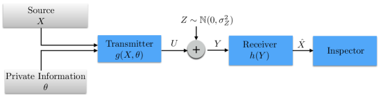
Figure 1: The problem setting

The privacy considerations have recently gained renewed interest, see e.g., [5, 6, 7] and the references therein. In [8, 9], Yamamoto studied a compression problem similar to the one considered here: find an encoder such that there exists a decoder that guarantees a distortion no larger than $D_{C}$ when measured with $\rho_{C}$ and at the same time cannot be smaller than $D_{P}$, when measured with $\rho_{P}$ in conjunction with any other decoder. In [7], Yamamoto’s result was extended to some special cases to analyze the privacy-utility tradeoff in databases.

In this paper, we explicitly study the equilibrium conditions under transmitter’s privacy constraints. The contributions of this paper are:

• We first formulate the problem, that involves minimization of a global objective by the encoder and the decoder subject to a privacy constraint measured by a different function.

• Assuming an entropy based privacy measure and quadratic distortion measure, we characterize the achievable distortion-privacy region with or without compression at the transmitter.

• We study the impact of the presence of an average power constrained Gaussian communication channel on the privacy-distortion trade-off.

II Preliminaries

II-A Notation

Let $\mathbb{R}$ and $\mathbb{R}^{+}$ denote the respective sets of real numbers and positive real numbers. Let $\mathbb{E}(\cdot)$ denote the expectation operator. The Gaussian density with mean $\mu$ and variance $\sigma^{2}$ is denoted as $\mathcal{N}(\mu,\sigma^{2})$. All logarithms in the paper are natural logarithms and may in general be complex valued, and the integrals are, in general, Lebesgue integrals. Let us define ${\cal{S}}$ to denote the set of Borel measurable, square integrable functions $\{{f}:\mathbb{R}\rightarrow\mathbb{R}$}. For information theoretic quantities, we use standard notations as, for example, in [10]. We let $H(X)$ and $I(X;Y)$ denote the entropy of a discrete random variable $X$(or differential entropy if $X$ is continuous), and the mutual information between the random variables $X$ and $Y$, respectively.

II-B Setting-1: Simple Equilibrium

We consider the general communication system whose block diagram is shown in Figure 1. The source $X$ and private information $\theta$ are mapped into ${Y}\in\mathbb{R}$ which is fully determined by the conditional distribution $p(\cdot|x,\theta)$. For the sake of brevity, and with a slight abuse of notation, we refer to this as a stochastic mapping $Y=g(X,\theta)$ so that

$$\mathbb{P}(g(X,\theta)\in{\cal Y})=\int\limits_{y^{\prime}\in{\cal Y}}p(y^{\prime}|x,\theta)\mathrm{d}x\mathrm{d}\theta\,\,\quad\forall{\cal Y}\subseteq\mathbb{R}$$ (1)

holds almost everywhere in $X$ and $\theta$. Let the set of all such mappings be denoted by $\Gamma$ (which has a one-to-one correspondence to the set of all the conditional distributions that construct the transmitter output $Y$).

The receiver produces an estimate of the source ${\hat{X}}$ through a mapping $h\in{\cal S}$ as ${\hat{X}}=h(Y)$. An inspector observes the estimate of the receiver, aims to learn about the private information $\theta$, i.e., minimize $H(\theta|\hat{X})$. Note that the joint statistics of the random variables is common knowledge. The common objective of the transmitter and the receiver is to minimize end-to-end distortion measured by a given distortion measure $\rho_{C}$ as

$$D_{C}=\mathbb{E}\{\rho_{C}(X,{\hat{X}})\}$$ (2)

over the mappings $g,h$ subject to a privacy constraint:

$$\mathbb{E}\{\rho_{P}(\theta,{\hat{X}})\}\geq J_{P}$$ (3)

over only the encoding mapping $g$ (the decoder is oblivious to the privacy objective). Here, the encoder aims to minimize $D_{C}$ in collaboration with the decoder (classical communication problem). The encoder has another objective, however: to maximize privacy, measured by, say $\rho_{P}$ or to guarantee that this privacy is not less than a given threshold, say $J_{P}\in\mathbb{R}^{+}$. Note that the decoder has no interest in finding out this information, or in satisfying or not satisfying this constraint. This subtle difference, i.e., the fact that there is a mismatch between the objectives of the decoder and those of the encoder, motivates us to consider this problem in a game theoretic setting (the SIT problem). In game theoretic terms, we consider a constrained Stackelberg game where only one of the players (the encoder) is concerned with the constraint in (3). Here, the encoder knows that the decoder will act to minimize the global cost $D_{C}$. Hence, Player 1 (leader) is the encoder and it knows that Player 2 (follower, the decoder) acts to minimize $D_{C}$. The leader (the encoder) acts to minimize $D_{C}$ subject to (3) knowing the decoder’s objective. In the following, we present this optimization problem formally:

Problem 1

Find $g(\cdot,\cdot)\in\Gamma$ which minimizes

$$\mathbb{E}\{\rho_{C}(X,h^{*}(g(X,\theta)))\}$$

subject to

$$\mathbb{E}\{\rho_{P}(\theta,h^{*}(g(X,\theta)))\}\geq J_{P}$$

where

$$h^{*}(g)=\operatorname*{argmin}\limits_{\begin{subarray}{c}h\end{subarray}\in{\cal S}}\mathbb{E}\{\rho_{C}(X,h(g(X,\theta))\}$$

In this paper, we specialize to quadratic Gaussian settings, i.e., the source and the private information are jointly Gaussian, the distortion measure is mean squared error and the privacy measure is conditional entropy. Particularly, this setting implies that $(X,\theta)\sim\mathcal{N}(0,R_{X\theta})$, where $R_{X\theta}=\sigma_{X}^{2}\left[\begin{array}[]{cc}1&\rho\\ \rho&r\end{array}\right]$; without loss of any generality we take $\rho\geq 0$, and naturally also $\rho^{2}\leq r$. Further, the distortion and privacy measures are given as follows:

$$\rho_{C}(x,y)=(x-y)^{2}$$ (4)

and

$$\rho_{P}(x,y)=-\log p(X|Y)$$ (5)

which results in conditional entropy as the privacy measure $\mathbb{E}\{\rho_{P}(x,y)\}=H(X|Y)$. The following lemma is a simple consequence of the fact that the Gaussian distribution maximizes entropy subject to covariance constraints (see [11]). This lemma will be used to convert the equilibrium conditions related to compression and communication problems to a control theoretic framework (an optimization problem involving second order statistics).

Lemma 1

At equilibrium, $Y,X,\theta$ are jointly Gaussian.

Lemma 1 ensures optimality of a linear decoder and hence $H(\theta|\hat{X})=H(\theta|Y)$ since $\hat{X}$ is an invertible function of $Y$. Note that invertibility of the decoding mapping, and hence this simplification in the privacy constraint is a direct consequence of the Stackelberg equilibrium. The Nash equilibrium variant of the same problem, studied in [1] without a privacy constraint, does not yield $H(\theta|\hat{X})=H(\theta|Y)$, since the decoding mapping at equilibrium is not invertible (quantizer based). Lemma 1 and the fact that maximizing $H(\xi_{1}|\xi_{2})$ is equivalent to maximizing $\mathbb{E}\{(\xi_{1}-\mathbb{E}\{\xi_{1}|\xi_{2}\})^{2}\}$ for jointly Gaussian $\xi_{1},\xi_{2}$, enable the following reformulation of Problem 1:

Problem 2

Find $Y=g(X,\theta)$ where $g(\cdot,\cdot)\in\Gamma$ minimizes

$$D_{C}=\mathbb{E}\{(X-\mathbb{E}\{X|Y\})^{2}\}$$

subject to

$$\mathbb{E}\{(\theta-\mathbb{E}\{\theta|Y\})^{2}\}\geq D_{P}$$

In this paper, we show the existence of such an equilibrium, and its essential uniqueness .

II-C Setting-2: Compression

Next, we consider the compression of the source $X$ subject to privacy constraints, and analyze this problem from an information theoretic perspective.

Formally, we consider an i.i.d. source $X^{n}$ and a private information sequence $\theta^{n}$ to be compressed to $M\approx 2^{nR}$ indices through $f_{E}$. The receiver applies a decoding function $f_{D}$ to generate the reconstruction sequence ${\hat{X}}^{n}$. Due to the strategic aspect of the problem, we have one distortion measure and one privacy measure. Similar to previous settings, we assume that the distortion is measured by MSE

$$D_{C}(f_{E},f_{D})=\frac{1}{n}\sum\limits_{i=1}^{n}\mathbb{E}\{(X_{i}-{\hat{X}}_{i})^{2}\},$$ (6)

and privacy is measured by conditional entropy.

$$J_{P}(f_{E},f_{D})=H(\theta^{n}|{\hat{X}^{n}})$$ (7)

A triple $(R,D_{C},J_{P})$ is called achievable if for every $\delta>0$ and sufficiently large $n$, there exists a block code $(f_{E},f_{D})$ such that

$$\frac{1}{n}\log{M} \leq R+\delta$$

$$D_{C}(f_{E},f_{D}) \leq D_{C}+\delta$$

$$J_{P}(f_{E},f_{D}) \leq J_{P}+\delta\;.$$

The set of achievable rate distortion triple $(R,D_{C},J_{P})$ is denoted here as ${\cal RD}$. The following theorem, whose proof directly follows from the arguments in [8] for a general distortion measure $d_{C}$ and conditional entropy, characterizes the achievable region ${\cal RD}_{S}$, i.e., converts the problem from an $n-$dimensional optimization to a single letter.

Theorem 1

${\cal RD}$ is the convex hull of triples $(R,D_{C},J_{P})$ for

$$R \geq I(X,\theta;Y)$$

for a conditional distribution $p(Y|X,\theta)$ and a deterministic decoding function $h:\mathbb{R}\rightarrow\mathbb{R}$ which satisfy

$$D_{C} \geq\mathbb{E}\{d_{C}(X,h(Y))\}$$

$$J_{P} \leq H(\theta|Y)$$

II-D Setting-3: Communication over Noisy Channel

Finally, we consider an additive Gaussian noise between the transmitter and the receiver. This problem setting is shown in Figure 1, where the receiver observes $Y=U+Z$, where $Z\sim\mathbb{N}(0,\sigma_{Z}^{2})$ is zero-mean Gaussian and distributed independent of $X$ and $\theta$. Again, we focus on entropy based privacy and quadratic distortion measure and Gaussian variables. The problem can then be reformulated as:

Problem 3

Find $U=g(X,\theta)$ that minimize

$$D_{C}=\mathbb{E}\{(X-\mathbb{E}\{X|Y\})^{2}\}$$

subject to

$$\mathbb{E}\{(\theta-\mathbb{E}\{\theta|Y\})^{2}\}\geq D_{P}$$

where $Y=U+Z$.

III Main Results

III-A Simple Equilibrium

Note that Lemma 1 does not provide the exact form of the function $g(\cdot,\cdot)\in\Gamma$, although it implies that $Y=X+\alpha\theta+S$ for some $\alpha\in\mathbb{R}$ and $S\sim\mathbb{N}(0,\sigma_{S}^{2})$ independent of $X$ and $\theta$. The following observation involves the two extreme cases of this problem, i.e., the endpoints of the $D_{C}$-$D_{P}$ curve.

Lemma 2

At maximum privacy, where $H(\theta|\hat{X})=H(\theta)$, and at minimum privacy, where $H(\theta|\hat{X})=H(\theta|X)$, the equilibrium is achieved at $Y=X+\alpha\theta$ for some $\alpha\in\mathbb{R}$. In other words, at end points, there is no need to have the noise term $S$.

Proof:

At minimum privacy, obviously the optimal transmitter strategy is $Y=X$ which results in $D_{C}=0$. The only way to achieve maximum privacy, $H(\theta|\hat{X})=H(\theta)$, is to render transmitter output $Y$ independent of $\theta$. Since variables are jointly Gaussian, this can be achieved by simply transmitting the prediction error, $Y=X+\alpha\theta$ where $\alpha=-\frac{\rho}{r}$ is MMSE prediction coefficient of $X$ from $\theta$. After prediction, the privacy constraint is satisfied and adding noise only increases $D_{C}$, hence $Y=X+\alpha\theta$ is the optimal transmitter strategy. ∎

In the following, we obtain auxiliary functional properties of $D_{C}$ and $D_{P}$ as a function of the encoding mapping $g(\cdot,\cdot)$ or equivalently $f_{Y|X,\theta}$ and the $D_{C}-D_{P}$ curve.

Lemma 3

$D_{C}$ and $D_{P}$ are concave functions of $f_{Y|X,\theta}$, and $D_{C}(D_{P})$ is an increasing, concave function of $D_{P}$.

Proof:

Let $Y^{(i)}$ be the random variables achieving $D_{C}(f^{(i)}_{Y|X,\theta})$ be characterized by $f_{Y|X,\theta}^{(i)}$, and $h^{(i)}$ for $i=1,2$.

For $0\leq c\leq 1$ we define

$$f^{c}_{Y|X,\theta}=cf^{(1)}_{Y|X,\theta}+(1-c)f^{(2)}_{Y|X,\theta}.$$

Then, for any decoding function $h^{(c)}(y)$

$$cD_{C}(f^{(1)}_{Y|X,\theta})+(1-c)D_{C}(f^{(2)}_{Y|X,\theta})$$

$$=c\int f_{X,\theta}(x,\theta)f^{(1)}_{Y|{X,\theta}}(x,\theta)(x-h^{(1)}(y))^{2}\mathrm{d}x\mathrm{d}\theta$$

$$+(1-c)\int f_{X,\theta}(x,\theta)f^{(2)}_{Y|X,\theta}(x,\theta)(x-h^{(2)}(y))^{2}\mathrm{d}x\mathrm{d}\theta$$

$$\leq c\int f_{X,\theta}(x,\theta)f^{(1)}_{Y|X}(x,y)(x-h^{(c)}(y))^{2}\mathrm{d}x\mathrm{d}\theta$$

$$+(1-c)\int f_{X,\theta}(x,\theta)f^{(2)}_{Y|X,\theta}(x,\theta)(x-h^{(c)}(y))^{2}\mathrm{d}x\mathrm{d}\theta$$

$$=\int f_{X,\theta}(x,\theta)(cf^{(1)}_{Y|X,\theta}(x,\theta)+(1-c)f^{(2)}_{Y|X,\theta}(x,\theta))$$

$$\quad\quad\quad\quad\quad\quad\quad\quad\quad\quad\quad(x-h^{(c)}(y))^{2}\mathrm{d}x\mathrm{d}\theta$$

$$=\int f_{X,\theta}(x,\theta)f^{c}_{Y|X,\theta}(x,\theta)(x-h^{(c)}(y))^{2}\mathrm{d}x\mathrm{d}\theta$$

$$=D_{C}(cf^{(1)}_{Y|X,\theta}+(1-c)f^{(2)}_{Y|X,\theta})$$ (8)

which shows the concavity of $D_{C}$ in $f_{Y|X,\theta}$. Following similar steps, we obtain concavity of $D_{P}$ in $f_{Y|X,\theta}$, i.e., we have

$$cD_{P}(f^{(1)}_{Y|X,\theta})+(1-c)D_{P}(f^{(2)}_{Y|X,\theta})\leq D_{P}(f^{c}_{Y|X,\theta})$$ (9)

Note that $D_{C}(D_{P})$ is non-decreasing since $D_{C}(D_{P})$ as expressed in Problem 2, is a minimization over a constraint set, as $D_{P}$ increases, minimization is performed over a smaller set, hence $D_{C}(D_{P})$ is non-decreasing.

Toward showing concavity of $D_{C}(D_{P})$, we first note that one can show concavity of $D_{C}$ in $f_{\hat{\theta},Y|X,\theta}$ where $\hat{\theta}$ is the inspector’s estimate of $\theta$, following similar steps to the preceding analysis. Then, let $Y^{(i)},{\hat{\theta}}^{(i)}$ be the random variables achieving $D_{C}(D_{P}^{(i)})$ be characterized by $f_{{\hat{\theta}},Y|X,\theta}^{(i)}$ for $i=1,2$. We need to show

$$D_{C}(cD_{P}^{(1)}+(1-c)D_{P}^{(2)})\geq cD_{C}(D_{P}^{(1)})+(1-c)D_{C}(D_{P}^{(2)})$$ (10)

for all $0\leq c\leq 1$.

$$cD_{C}(D_{P}^{(1)})+(1-c)D_{C}(D_{P}^{(2)})=$$

$$cD_{C}(f^{(1)}_{{\hat{\theta}},Y|X,\theta})+(1-c)D_{C}(f^{(2)}_{{\hat{\theta}},Y|X,\theta})$$ (11)

$$\leq D_{C}(cf^{(1)}_{{\hat{\theta}},Y|X,\theta}+(1-c)f^{(2)}_{{\hat{\theta}},Y|X,\theta})$$ (12)

$$=D_{C}(cD_{P}^{(1)}+(1-c)D_{P}^{(2)})$$ (13)

where the last step is due to the fact that $D_{P}$ is linear in $f_{\hat{\theta},Y|X,\theta}$.

Since both privacy and distortions measures are continuous, we only needed to show concavity, since monotonicity is a consequence of concavity and continuity. ∎

Lemma 2 describes the equilibrium conditions at the end points. The following theorem provides the exact characterization of this equilibrium over the entire $D_{P}-D_{C}$ region.

Theorem 2

For the quadratic Gaussian setting with entropy base privacy constraint, the (essentially) unique equilibrium is achieved by $g(X,\theta)=X+\alpha\theta$ and $h(Y)=\kappa Y$ where $\alpha$ and $\kappa$ are constants given as:

$$\alpha= -\frac{\rho}{r}\pm\sqrt{\left(1-\frac{\rho^{2}}{r}\right)\left(\frac{1}{r}-\frac{\sigma_{X}^{2}}{D_{P}}\right)}$$ (14)

$$\kappa= \frac{1+\alpha\rho}{1+\alpha^{2}r+2\alpha\rho}$$ (15)

Remark 1

An interesting aspect of the solution is that adding independent noise is strictly suboptimal in achieving the privacy-distortion trade-off.

Proof:

First, we note that the optimal decoder mapping is

$$h(Y)=\mathbb{E}\{X|Y\}$$ (16)

regardless of the choice of encoder’s policy $g(\cdot,\cdot)$. Hence, the problem simplifies to an optimization over the encoding mapping $g$.

Noting that at equilibrium $Y$ and $X,\theta$ are jointly Gaussian, without loss of generality, we take $Y=X+\alpha\theta+S$ where $S\sim\mathbb{N}(0,\sigma_{S}^{2})$ is independent of $X$ and $\theta$. In the following, we find the value of $\alpha$ and $\sigma_{S}^{2}$ at equilibrium. First, let us express $D_{C}$ and $D_{P}$ using standard estimation techniques:

$$D_{C}(\alpha,\sigma_{S}^{2})= \mathbb{E}\{(X-\mathbb{E}\{X|Y\})^{2}\}$$ (17)

$$= \sigma_{X}^{2}\left(1-\frac{(1+\alpha\rho)^{2}}{1+2\alpha\rho+\alpha^{2}r+\frac{\sigma_{S}^{2}}{\sigma_{X}^{2}}}\right)$$ (18)

$$D_{P}(\alpha,\sigma_{S}^{2})= \mathbb{E}\{(\theta-\mathbb{E}\{\theta|Y\})^{2}\}$$ (19)

$$= \sigma_{X}^{2}\left(r-\frac{(\rho+r\alpha)^{2}}{1+2\alpha\rho+\alpha^{2}r+\frac{\sigma_{S}^{2}}{\sigma_{X}^{2}}}\right)$$ (20)

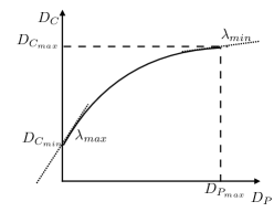
Figure 2: $D_{P}-D_{C}$ curve

Problem 1 can now be converted to an unconstrained [12] minimization of the Lagrangian cost:

$$J(\alpha,\sigma_{S}^{2})=D_{C}(\alpha,\sigma_{S}^{2})-\lambda D_{P}(\alpha,\sigma_{S}^{2})$$ (21)

for where varying $\lambda\in\mathbb{R}^{+}$ provides solutions at different levels of privacy constraint $D_{P}$. A set of necessary conditions for optimality can be obtained by applying K.K.T. conditions, one of which is that $\lambda$ is the slope of the curve:

$$\lambda=\frac{dD_{C}(\alpha^{*},\sigma_{S}^{2*})}{dD_{P}(\alpha^{*},\sigma_{S}^{2*})}$$ (22)

at the optimal values of $\alpha$ and $\sigma_{S}^{2}$. Let us expand $J(\alpha,\sigma_{S}^{2})$

$$J(\alpha,\sigma_{S}^{2})=\sigma_{X}^{2}(1-\lambda r)-\sigma_{X}^{2}\left(\frac{(1+\alpha\rho)^{2}-\lambda(\rho+r\alpha)^{2}}{1+2\alpha\rho+\alpha^{2}r+\frac{\sigma_{S}^{2}}{\sigma_{X}^{2}}}\right)$$

The value of $\sigma_{S}^{2*}$ depends on the sign of $\Xi\triangleq\lambda(\rho+r\alpha)^{2}-(1+\alpha\rho)^{2}$, i.e., if $\Xi\geq 0$, then $\sigma_{S}^{2*}=0$. In the following, we show that $\Xi\geq 0$ for all $\alpha\in[-\frac{\rho}{r},0]$, and hence $\sigma_{S}^{2*}=0$.

First, we note that the minimum value of $\lambda$ is reached at the maximum allowed $D_{P}$, as depicted in Figure 2. From Lemma 2 for $D_{P}=D_{P_{max}}$, the solution implies that $\sigma_{S}^{2*}=0$. Hence, $\Xi\geq 0$ at $D_{P}=D_{P_{max}}$. Plugging the values, we obtain $\lambda\geq 0$. Following similar steps for $D_{P}=D_{P_{min}}$, we obtain $\lambda\leq\frac{1}{\rho^{2}}$. For $\lambda\in[0,\frac{1}{\rho^{2}}]$ and $\alpha\in[-\frac{\rho}{r},0]$, we have

$$\Xi\triangleq (1+\alpha\rho)^{2}-\lambda(\rho+\alpha)^{2}$$

$$\geq (1+\alpha\rho)^{2}-\frac{1}{\rho^{2}}(\rho+\alpha)^{2}$$

$$= 2\alpha(\rho-\frac{r}{\rho})+\alpha^{2}(\rho^{2}-\frac{r^{2}}{\rho^{2}})$$

$$= \alpha(\rho-\frac{r}{\rho})(2+\alpha(\rho+\frac{r}{\rho})).$$ (23)

Note that from Cauchy-Schwarz inequality, we have $r\geq\rho^{2}$ and noting that $-\frac{\rho}{r}\geq\alpha\geq 0$, we conclude $\Xi\geq 0$. Hence, $\sigma_{S}^{2*}=0$ for all values of $D_{P}$. Toward obtaining $\alpha^{*}$, plug $\sigma_{N}^{2}=0$ into (20), to obtain:

$$\left(1-\frac{r-\rho^{2}}{D_{P}/\sigma_{X}^{2}}\right)+2\alpha\rho+\alpha^{2}r=0.$$

The solution to this second order equation is simply

$$\alpha^{*}=-\frac{\rho}{r}\pm\sqrt{\left(1-\frac{\rho^{2}}{r}\right)\left(\frac{1}{r}-\frac{\sigma_{X}^{2}}{D_{P}}\right)}$$ (24)

Both of these solutions (corresponding to $\pm$) satisfy the privacy constraint with equality, and the following one achieves lower $D_{C}$, and hence is the optimal solution:

$$\alpha^{*}=-\frac{\rho}{r}+\sqrt{\left(1-\frac{\rho^{2}}{r}\right)\left(\frac{1}{r}-\frac{\sigma_{X}^{2}}{D_{P}}\right)}$$ (25)

The optimal decoding mapping is

$$h(Y)=\mathbb{E}\{X|Y\}= \frac{1+\alpha\rho}{1+r\alpha^{2}+2\alpha\rho}Y.$$ (26)

∎

III-B Problem-2

Next, we consider compression of jointly Gaussian source-private information with entropy based privacy measure and MSE distortion. First, we observe that all equilibrium points are achieved by a jointly Gaussian $X,\theta,Y$ and hence $Y$ can be written as $Y=X+\alpha\theta+N$ for some $\alpha\in\mathbb{R}$, and $N\sim\mathbb{N}(0,\sigma_{N}^{2})$ is Gaussian and independent of $X$ and $\theta$.

The proof of this statement follows from the well-known property of Gaussian distribution achieving maximum entropy under a variance constraint and the steps in the proof of Theorem 1. Hence, the test channel achieving the rate-distortion function adds independent Gaussian noise (forward test channel interpretation of Gaussian rate distortion also holds in this privacy constrained setting). Note that the privacy constraint is always active in the simple equilibrium setting, and the equilibrium is at the boundary of the constraint set, i.e., we find optimal $\alpha$ by setting the privacy constraint equality. In the compression case, compression itself provides some level privacy inherently (it is evident from the forward channel interpretation of the RD function). Hence, the privacy constraint may not be active in the compression case, which yields $\alpha^{*}=0$. The following theorem characterizes the optimal rate-distortion-privacy trade-off.

Theorem 3

For a given $D_{P}$, the space of $R-D_{C}$ is given as

$$R= \log\left(1+\frac{\sigma_{X}^{2}}{\sigma_{N}^{2}}(1+\alpha^{2}r+2\alpha\rho)\right)$$ (27)

$$D_{C}= \sigma_{X}^{2}\left(1-\frac{(1+\alpha\rho)^{2}}{1+2\alpha\rho+\alpha^{2}r+\frac{\sigma_{N}^{2}}{\sigma_{X}^{2}}}\right)$$ (28)

where

$$\alpha=-\frac{\rho}{r}+\Phi,$$ (29)

and

$$\Phi=\min\left(\sqrt{\left(1-\frac{\rho^{2}}{r}\right)\left(\frac{1}{r}-\frac{1}{\frac{D_{P}}{\sigma_{X}^{2}}(1+\sigma_{N}^{2})-r\sigma_{N}^{2}}\right)},\frac{\rho}{r}\right)$$

as a function of $\sigma_{N}^{2}$.

Proof:

We have $Y=X+\beta\theta+N$ for some $\alpha\in\mathbb{R}$ where $N$ is zero-mean Gaussian with variance $\sigma_{N}^{2}$ and independent of $X$ and $\theta$. This representation yields, by standard estimation theoretic techniques, the following characterization of $R,D_{C},D_{P}$ in terms of $\sigma_{N}^{2}$:

$$R =\frac{1}{2}\log\left(1+\frac{\sigma_{X}^{2}}{\sigma_{N}^{2}}(1+\alpha^{2}r+2\alpha\rho)\right)$$ (30)

$$D_{C} =\sigma_{X}^{2}\left(\frac{\alpha^{2}(r-\rho^{2})+\frac{\sigma_{N}^{2}}{\sigma_{X}^{2}}}{1+2\alpha\rho+\alpha^{2}r+\frac{\sigma_{N}^{2}}{\sigma_{X}^{2}}}\right)$$ (31)

$$D_{P} =\sigma_{X}^{2}\left(r-\frac{(\rho+r\alpha)^{2}}{1+2\alpha\rho+\alpha^{2}r+\frac{\sigma_{N}^{2}}{\sigma_{X}^{2}}}\right)$$ (32)

Following steps similar to the ones in the proof of Theorem 2, we can express $\alpha^{*}$ in terms of $D_{P}$, when the privacy constraint is active, as:

$$\alpha^{*}=-\frac{\rho}{r}\pm\sqrt{\left(1-\frac{\rho^{2}}{r}\right)\left(\frac{1}{r}-\frac{1}{\frac{D_{P}}{\sigma_{X}^{2}}(1+\sigma_{N}^{\prime 2})-r\sigma_{N}^{2}}\right)}.$$

Form these solutions, the following achieves a lower value for $D_{C}$:

$$\alpha^{*}=-\frac{\rho}{r}+\sqrt{\left(1-\frac{\rho^{2}}{r}\right)\left(\frac{1}{r}-\frac{1}{\frac{D_{P}}{\sigma_{X}^{2}}(1+\sigma_{N}^{\prime 2})-r\sigma_{N}^{2}}\right)}.$$

When the privacy constraint is already satisfied, $\alpha^{*}=0$.

∎

III-C Problem-3

We next focus on noisy communication settings, i.e., we assume there is an additive white Gaussian noise $Z\sim\mathbb{N}(0,\sigma_{Z}^{2})$ as shown in Figure 2. The following theorem provides the encoding and decoding mappings at the equilibirum.

Theorem 4

For the quadratic Gaussian communication setting with entropy based privacy constraint, the (essentially) unique equilibrium is achieved by

$$U=\sqrt{\frac{P_{T}}{\sigma_{X}^{2}(1+2\alpha\rho+\alpha^{2}r)}}(X+\alpha\theta)$$

and $h(Y)=\kappa Y$ where $\alpha$ and $\kappa$ are constants given as:

$$\kappa= \frac{1+\alpha\rho}{1+\alpha^{2}r+2\alpha\rho}$$ (33)

and

$$\alpha=-\frac{\rho}{r}+\Phi,$$ (34)

and

$$\Phi=\min\left(\sqrt{\left(1-\frac{\rho^{2}}{r}\right)\left(\frac{1}{r}-\frac{1}{\frac{D_{P}}{\sigma_{X}^{2}}(1+\sigma_{N}^{2})-r\sigma_{N}^{2}}\right)},\frac{\rho}{r}\right)$$

Proof:

First, we observe that linear mappings are optimal, due to the well-known optimality of linear mappings (without the privacy constraint) [13], and the fact that jointly Gaussian $U,X,\theta$ maximizes $H(\theta|Y)$ with fixed second-order statistics. Next, we assume without any loss of generality, that $Y=\beta(X+\alpha\theta)+N$ for some $\beta\in\mathbb{R}^{+}$ and $\alpha\in\mathbb{R}$. Then, we have

$$\mathbb{E}\{XY\}=\beta\sigma_{X}^{2}(1+\alpha\rho), \quad\mathbb{E}\{\theta Y\}=\beta\sigma_{X}^{2}(\rho+r\alpha)$$

$$\mathbb{E}\{Y^{2}\} =\beta^{2}\sigma_{X}^{2}(1+2\alpha\rho+r\alpha^{2})+\sigma_{N}^{2}$$

Hence,

$$D_{P}= \sigma_{X}^{2}\left(r-\frac{(\rho+r\alpha)^{2}}{1+2\alpha\rho+\alpha^{2}r+\frac{\sigma_{N}^{2}}{\beta^{2}\sigma_{X}^{2}}}\right)$$ (35)

$$D_{C}= \sigma_{X}^{2}\left(1-\frac{(1+\alpha\rho)^{2}}{1+2\alpha\rho+\alpha^{2}r+\frac{\sigma_{N}^{2}}{\beta^{2}\sigma_{X}^{2}}}\right)$$ (36)

Note that since $P_{T}=\mathbb{E}\{U^{2}\}=\beta^{2}\sigma_{X}^{2}(1+2\alpha\rho+\alpha^{2}r)$, we can re-express $D_{P}$ as

$$D_{P}= \sigma_{X}^{2}\left(r-\frac{\beta^{2}\sigma_{X}^{2}(\rho+r\alpha)^{2}}{P_{T}+\sigma_{N}^{2}}\right)$$ (37)

$$= \sigma_{X}^{2}\left(r-\frac{(\rho+r\alpha)^{2}}{1+2\alpha\rho+\alpha^{2}r}\frac{P_{T}}{P_{T}+\sigma_{N}^{2}}\right)$$ (38)

$$= \sigma_{X}^{2}\left(\frac{\sigma_{N}^{2}}{P_{T}+\sigma_{N}^{2}}r+\frac{r-\rho^{2}}{1+2\alpha\rho+\alpha^{2}r}\frac{P_{T}}{P_{T}+\sigma_{N}^{2}}\right)$$ (39)

Note that the power constraint is always active, and when the privacy constraint is active, we have:

$$\alpha^{*}\!=-\!\frac{\rho}{r}\!\pm\sqrt{\left(\!1\!-\!\frac{\rho^{2}}{r}\right)\left(\frac{1}{r}\!-\!\frac{1}{\frac{D_{P}}{\sigma_{X}^{2}}(\!1\!+\!\sigma_{N}^{2}/P_{T})\!-\!r\sigma_{N}^{2}/P_{T}}\right)}.$$

From these solutions, the following achieves a lower $D_{C}$:

$$\alpha^{*}\!=\!-\frac{\rho}{r}+\sqrt{\left(1\!-\!\frac{\rho^{2}}{r}\right)\left(\frac{1}{r}\!-\!\frac{1}{\frac{D_{P}}{\sigma_{X}^{2}}(\!1\!+\!\sigma_{N}^{2}/P_{T})\!-\!r\sigma_{N}^{2}/P_{T}}\right)}.$$

When the privacy constraint is already satisfied, $\alpha^{*}=0$. ∎

IV Conclusion

In this paper, we have addressed some fundamental problems associated with strategic communication in the presence of privacy constraints. Although the compression and communication problems are inherently information theoretic, for entropy based privacy measure, MSE distortion and jointly Gaussian source and private information, the problem admits a control theoretic representation (optimization over second order statistics). We have explicitly characterized the equilibrium conditions for compression and communication under privacy constraints. Rather surprisingly, the simple equilibrium solution (without compression) does not require addition of independent noise to satisfy the privacy constraints, as opposed to the common folklore in such problems. Some future directions include using results presented in this paper for decentralized stochastic control problems (see [14]) with privacy constraints, extending the approach to vector and network settings, and finally investigating implications in economics.

References

• [1] V. Crawford and J. Sobel, “Strategic information transmission,” Econometrica: Journal of the Econometric Society, pp. 1431–1451, 1982.
• [2] M. Battaglini, “Multiple referrals and multidimensional cheap talk,” Econometrica, vol. 70, no. 4, pp. 1379–1401, 2002.
• [3] T. Başar and G. Olsder, Dynamic Noncooperative Game Theory, Society for Industrial Mathematics (SIAM) Series in Classics in Applied Mathematics, 1999.
• [4] F. Farokhi, A. Teixeira, and C. Langbort, “Estimation with strategic sensors,” arXiv:1402.4031, 2014.
• [5] C. Dwork, “Differential privacy,” in Encyclopedia of Cryptography and Security, pp. 338–340. Springer, 2011.
• [6] F. McSherry and K. Talwar, “Mechanism design via differential privacy,” in Foundations of Computer Science, 2007. FOCS’07. 48th Annual IEEE Symposium on. IEEE, 2007, pp. 94–103.
• [7] L. Sankar, R. Rajagopalan, and H. V. Poor, “Utility-privacy tradeoffs in databases: An information-theoretic approach,” IEEE Transactions on Information Forensics and Security, vol. 8, no. 6, pp. 838–852, 2013.
• [8] H. Yamamoto, “A rate-distortion problem for a communication system with a secondary decoder to be hindered,” IEEE Transactions on Information Theory, vol. 34, no. 4, pp. 835–842, 1988.
• [9] H. Yamamoto, “A source coding problem for sources with additional outputs to keep secret from the receiver or wiretappers (corresp.),” IEEE Transactions on Information Theory,, vol. 29, no. 6, pp. 918–923, Nov 1983.
• [10] T. Cover and J. Thomas, Elements of Information Theory, John Wiley & Sons, 2012.
• [11] S. N. Diggavi and T. M. Cover, “The worst additive noise under a covariance constraint,” IEEE Transactions on Information Theory, vol. 47, no. 7, pp. 3072–3081, Nov 2001.
• [12] S. Boyd and L. Vandenberghe, Convex Optimization, Cambridge University Press, 2004.
• [13] T. Goblick Jr, “Theoretical limitations on the transmission of data from analog sources,” IEEE Transactions on Information Theory, vol. 11, no. 4, pp. 558–567, 1965.
• [14] R. Bansal and T. Başar, “Stochastic teams with nonclassical information revisited: When is an affine law optimal?,” IEEE Transactions on Automatic Control, vol. 32, no. 6, pp. 554–559, 1987.