Comparison of cosmological models using standard rulers and candles

Abstract

In this paper, we used standard rulers and standard candles (separately and jointly) to explore five popular dark energy models under assumption of spatial flatness of the Universe. As standard rulers, we used a data set comprising 118 galactic-scale strong lensing systems (individual standard rulers if properly calibrated for the mass density profile) combined with BAO diagnostics (statistical standard ruler). Supernovae Ia served as standard candles. Unlike in the most of previous statistical studies involving strong lensing systems, we relaxed the assumption of singular isothermal sphere (SIS) in favor of its generalization: the power-law mass density profile. Therefore, along with cosmological model parameters we fitted the power law index and its first derivative with respect to the redshift (thus allowing for mass density profile evolution). It turned out that the best fitted $\gamma$ parameters are in agreement with each other irrespective of the cosmological model considered. This demonstrates that galactic strong lensing systems may provide a complementary probe to test the properties of dark energy. Fits for cosmological model parameters which we obtained are in agreement with alternative studies performed by the others. Because standard rulers and standard candles have different parameter degeneracies, combination of standard rulers and standard candles gives much more restrictive results for cosmological parameters. At last, we attempted at model selection based on information theoretic criteria (AIC and BIC). Our results support the claim, that cosmological constant model is still the best one and there is no (at least statistical) reason to prefer any other more complex model.

1 Introduction

One of the most important issues in modern cosmology is the accelerated expansion of the universe, deduced from Type Ia supernovae (Riess et al., 1998; Perlmutter et al., 1999) and also confirmed by other independent probes, such as Cosmic Microwave Background (CMB)(Pope et al., 2004) and the Large Scale Structure (LSS) (Spergel et al., 2003). In order to explain this phenomenon, a new component, called dark energy, which fuels the cosmic acceleration due to its negative pressure and may dominate the universe at late times has been introduced.

Although cosmological constant $\Lambda$ (Peebles & Ratra, 2003), the simplest candidate for dark energy, seems to fit in with current observations, yet it suffers from the well-known fine tuning and coincidence problems. Therefore a variety of dark energy models, including different dark energy equation of state (EoS) parametrizations such as XCDM model (Ratra et al., 1988), and Chevalier-Polarski-Linder (CPL) model (Chevalier & Polarski, 2001; Linder, 2004) have been put forward, each of which has its own advantages and problems in explaining the acceleration of the universe. Yet, the nature of dark energy still remains unknown. It might also be possible that observed accelerated expansion of the Universe is due to departures of the true theory of gravity from General Relativity, e.g. due to quantum nature of gravity or possible multidimensionality of the world. Hence such models like Dvali-Gabadadze-Porrati – inspired by brane theory or Ricci dark energy inspired by the holographic principle have been proposed. Having no clear preference from the side of theory and in order to learn more about dark energy, we have to turn to the sequential upgrading of observational fits of quantities which parametrize the unknown properties of dark energy (such as density parameters or coefficients in the cosmic equation of state) and seeking coherence among alternative tests. In this paper we highlight the usefulness of strong lensing systems to assess the parameters of several popular dark energy models. Because strong lensing systems are sensitive to angular diameter distance we supplement our analysis with Baryon Acoustic Oscillations (BAO) data and compare our results with the inference made using luminosity distances measured with SN Ia.

Strong gravitational lensing has recently developed into a serious technique in extragalactic astronomy (galactic structure studies) and in cosmology. First of all, the angular separation between images (determined by the Einstein radius of the lens) can be used to constrain and model the mass distribution of lens (Narayan & Bartelmann, 1996). Secondly, time delay between images are additional sources of constraints on the mass distribution of the lens. Strong lensing time delays have recently developed into a promising new technique to constrain cosmological parameters – the Hubble constant in the first place (Suyu et al., 2009). Finally, strong lensing systems are becoming an important tool in cosmology. Earlier attempts to use such systems for constraining cosmological parameters were based on comparison between theoretical (depending on the cosmological model) and empirical distributions of image separations (Chae et al., 2002; Cao & Zhu, 2012) or lens redshifts (Ofek et al., 2003; Cao, Covone & Zhu, 2012) in observed samples of lenses. Another approach is based on the fact that image separations in the system depend on angular diameter distances to the lens and to the source, which in turn are determined by background cosmology. This method applied in the context of dark energy was first proposed in the papers of Futamase & Yoshida (2001); Biesiada (2006); Gilmore & Natarayan (2009) and further developed in recent works (Biesiada, Piórkowska, & Malec, 2010; Cao et al., 2012).

However, there are two well known challenges to this method as a cosmological probe. The first issue is that detailed mass distribution of the lens and its possible evolution in time are not clear enough. The second challenge is the limited number of observed gravitational lensing systems with complete spectroscopic and astrometric information necessary for this technique. It is only quite recently when reasonable catalogs of strong lensing systems are becoming available. In this paper, we use an approach proposed by Cao et al. (2015a) where the lensing galaxy is assumed to have spherically symmetric mass distribution described by the power-law slope factor which is allowed to evolve with redshift.

Baryon Acoustic Oscillations (BAO) and strong lensing systems together, constitute such independent standard rulers which may have different degeneracies in the parameter space of dark energy models (Biesiada et al., 2011). Moreover, we also take supernovae Ia for comparison as an independent probe (standard candles). In Section 3, we present cosmological models considered and the corresponding results. In order to compare dark energy models with different numbers of parameters and decide which model is preferred by the current data, in Section 4 we apply two model selection techniques i.e. the Akaike Criterion (AIC) and Bayesian Information Criterion (BIC). Finally the results are summarized in Section 5.

2 Method and data

2.1 Strong lensing systems

Strong lensing system with the intervening galaxy acting as a lens usually produces multiple images of the source. Image separation depends in the first place on the mass of the lens (suitably parametrized by stellar velocity dispersion) but also on the angular diameter distances between the lens and the source and between the observer and the lens. Angular diameter distance between two objects at redshifts $z_{1}$ and $z_{2}$ respectively, is determined by background cosmology:

$${D(z_{1},z_{2};\bf{p})}={\frac{c}{{H_{0}}({1+z_{2})}}}{\int_{z_{1}}^{z_{2}}{\frac{dz}{E(z;\bf{p})}}}$$ (1)

where $E(z;\mathbf{p})=H(z;\mathbf{p})/H_{0}$ is the dimensionless expansion rate, $H_{0}$ is the Hubble constant and $\bf{p}$ denotes the parameters of a particular cosmological model considered.

Under assumption of the singular isothermal sphere (SIS) model, which so far was a standard one for elliptical galaxies acting as lenses, the Einstein radius $\theta_{E}$ is given by

$${{\theta}_{E}}=4{\pi}{\frac{D_{ls}}{D_{s}}}{\frac{{\sigma}^{2}_{SIS}}{c^{2}}}$$ (2)

where $D_{ls}$ and $D_{s}$ are angular diameter distances between lensing galaxy and the source and between the observer and the source, respectively. If the Einstein radius and the velocity dispersion of lensing galaxy are known from observations, the ratio of angular diameter distances $D_{ls}/D_{s}$ can be obtained from Eq. (2). The main challenge here is how to get the velocity dispersion of lensing galaxy $\sigma_{SIS}$ (which is the SIS model parameter) from central stellar velocity dispersion $\sigma_{0}$ obtained from spectroscopy. Previous analysis using strong gravitational lensing systems, took the phenomenological approach to relate these two velocity dispersions through $\sigma_{SIS}=f_{E}\sigma_{0}$, where $f_{E}$ was a free parameter with $0.8<f_{E}^{2}<1.2$ (Ofek et al., 2003; Cao et al., 2012).

In this paper, we generalize the SIS model to spherically symmetric power-law mass distribution $\rho\sim r^{-\gamma}$ (Cao et al., 2015a). Accordingly, the Einstein radius can be rewritten as

$${{\theta}_{E}}=4{\pi}{\frac{D_{ls}}{D_{s}}}{\frac{{\sigma}^{2}_{ap}}{c^{2}}}\left(\frac{{\theta}_{E}}{{\theta}_{ap}}\right)^{2-\gamma}f(\gamma)$$ (3)

where $\sigma_{ap}$ is the velocity dispersion inside the aperture of size ${\theta}_{ap}$, and

$${f(\gamma)}=-{\frac{1}{\sqrt{\pi}}}{\frac{(5-2{\gamma})(1-{\gamma})}{3-{\gamma}}}{\frac{\Gamma(\gamma-1)}{\Gamma(\gamma-{\frac{2}{3})}}}\left[\frac{(\Gamma(\frac{\gamma}{2})-\frac{1}{2})}{\Gamma(\frac{\gamma}{2})}\right]^{2}$$ (4)

As a result, observational value of the angular diameter distance ratio reads:

$${D^{obs}}={\frac{D_{ls}}{{D_{s}}}}={\frac{{c^{2}}{\theta_{E}}}{4{\pi}{{\sigma}^{2}_{ap}}}}\left(\frac{\theta_{ap}}{\theta_{E}}\right)^{2-\gamma}{f^{-1}(\gamma)}$$ (5)

and its theoretical counterpart can be obtained from Eq. (1)

$${D^{th}(z_{l},z_{s};\bf{p})}={\frac{D_{ls}{\bf{(p)}}}{D_{s}\bf{(p)}}}={\frac{{\int_{z_{l}}^{z_{s}}{\frac{dz}{E(z;\bf{p})}}}}{{\int_{0}^{z_{s}}{\frac{dz}{E(z;\bf{p})}}}}}$$ (6)

Then one can constrain cosmological models by minimizing the $\chi^{2}$ function given by

$${\chi^{2}_{SL}\bf{(p)}}=\sum^{N}_{i=1}\left[\frac{{D^{th}(z_{l,i},z_{s,i};\bf{p})}-{D^{obs}(\sigma_{ap,i},\theta_{E,i};\gamma)}}{\sigma_{D,i}}\right]^{2}$$ (7)

where the variance of $D^{obs}$ is

$${{\sigma^{2}_{D,i}}}=D^{obs}(\sigma_{ap,i},\theta_{E,i};\gamma)^{2}\left[4\left(\frac{\sigma_{\sigma_{ap}}}{\sigma_{ap}}\right)^{2}+{(1-\gamma)}^{2}\left(\frac{\sigma_{\theta_{E}}}{\theta_{E}}\right)^{2}\right].$$ (8)

In order to calculate $\sigma_{D}$, we assumed the fractional uncertainty of the Einstein radius at the level of $5\%$ (i.e., $\frac{\sigma_{\theta_{E}}}{\theta_{E}}$=0.05) for all the lenses, uncertainties of the velocity dispersion were taken from the data set — see (Cao et al., 2015a) for details.

We treated the mass density power-law index of lensing galaxies as a free parameter to be estimated together with cosmological parameters. Moreover, since it has recently been claimed that $\gamma$ index of elliptical galaxies might evolved with redshift (Ruff et al., 2011), we assumed the linear relation for $\gamma$: $\gamma=\gamma_{0}+\gamma_{1}z_{l}$. Furthermore, when dealing with a sample of lenses instead of a single lens system, we followed the standard practice and transformed velocity dispersion measured within actual circular aperture to the one within circular aperture of radius $R_{eff}/2$ (half the effective radius) according to the prescription of (Jorgensen et al., 1995): $\sigma_{0}=\sigma_{ap}{(\theta_{eff}/(2\theta_{ap}))}^{-0.04}$. Such procedure has an advantage of standardizing measured velocity dispersions within the sample and introduces negligible terms to the error budget — for details see Cao et al. (2015a).

In this paper, we use a combined sample of $n=118$ strong lensing systems from SLACS (57 lenses taken from Bolton et al. (2008); Auger et al. (2009)), BELLS (25 lenses taken from Brownstein et al. (2012)), LSD (5 lenses from Treu & Koopmans (2002); Koopmans & Treu (2002); Treu & Koopmans (2004)) and SL2S (31 lenses taken from Sonnenfeld et al. (2013a, b)), which is the most recent compilation of galactic scale strong lensing data. This sample is compiled and summarized in Table 1 of Cao et al. (2015a), in which all relevant information necessary to perform cosmological model fit can be found.

2.2 Baryon Acoustic Oscillations

Baryon Acoustic Oscillations (BAO) refer to regular, periodic fluctuations in the density of visible baryonic matter in the Universe (the large scale structure). Being “the statistical standard ruler” they are commonly used to investigate dark energy. From BAO observations, we used the BAO distance ratio $r_{s}(z_{d})/D_{V}(z)$ measured by the Sloan Digital Sky Survey (SDSS) data release 7 (DR7) (Padmanabhan et al., 2012), SDSS-III Baryon Oscillation Spectroscopic Survey (BOSS) (Anderson et al., 2012), the clustering of WiggleZ survey (Blake et al., 2012) and 6dFGS survey (Beutler et al., 2011):

$$d_{z}=\frac{r_{s}(z_{d})}{D_{V}(z)}.$$ (9)

The meaning of the quantities $r_{s}(z_{d})$ and $D_{V}(z)$ is explained below. The effective distance is given by

$$D_{V}(z)\equiv[(1+z)^{2}D^{2}_{A}(z)\frac{cz}{H(z)}]^{1/3}$$ (10)

where $D_{A}(z)$ is the angular diameter distance and $H(z)$ is the Hubble parameter. The comoving sound horizon scale at the baryon drag epoch is

$$r_{s}(z_{d})=\int^{\infty}_{z_{d}}\frac{c_{s}(z^{\prime})dz^{\prime}}{E(z^{\prime})}$$ (11)

where the sound speed is given by the formula: $c_{s}(z)=1/\sqrt{3[1+\bar{R_{b}}/(1+z)]}$ where $\bar{R_{b}}=3\Omega_{b}h^{2}/(4\times 2.469\times 10^{-5})$, and the drag epoch redshift is fitted as

$$z_{d}=\frac{1291(\Omega_{m}h^{2})^{0.251}}{1+0.659(\Omega_{m}h^{2})^{0.828}}[1+b_{1}(\Omega_{b}h^{2})^{b_{2}}]$$ (12)

where $b_{1}=0.313(\Omega_{m}h^{2})^{-0.419}[1+0.607(\Omega_{m}h^{2})^{0.674}]$ and $b_{2}=0.238(\Omega_{m}h^{2})^{0.233}$.

The $\chi^{2}$ function for BAO data is defined as

$$\chi^{2}_{BAO}=\bf(x-d)^{T}(C_{BAO}^{-1})(x-d),$$ (13)

where

$${\bf{x-d}}=[r_{s}/D_{V}(0.1)-0.336,D_{V}(0.35)/r_{s}-8.88,$$ (14)

$$D_{V}(0.57)/r_{s}-13.67,r_{s}/D_{V}(0.44)-0.0916,$$

$$r_{s}/D_{V}(0.60)-0.0726,r_{s}/D_{V}(0.73)-0.0592]$$

and $C^{-1}_{BAO}$ is the corresponding inverse covariance matrix taken after Hinshaw et al. (2013). In order to constrain cosmological parameters with standard rulers, i.e. strong lensing systems and BAO we used the joint $\chi^{2}$ defined as:

$$\chi^{2}_{SL+BAO}={\chi^{2}_{SL}}+{\chi^{2}_{BAO}}$$ (15)

2.3 Supernovae Ia

Up to now, we discussed standard rulers, but it were standard candles (SN Ia) which kicked off the story of accelerated expansion of the Universe. Since then they remained a reference point for discussions and tests of cosmological models. Because standard rulers (SL+BAO) and standard candles measure the distances based on different concepts, cosmological inferences based on them have different degeneracies in parameter space. Therefore, we also considered constraints on cosmologies coming from SN Ia observations: for comparison and also for the sake of complementarity. In this paper, we used the latest Union2.1 compilation released by the Supernova Cosmology Project Collaboration consisting of 580 SN Ia data points (Suzuki et al., 2012), taking into consideration systematic errors of the observed distance modulus (Cao & Zhu, 2014). The Hubble constant $H_{0}$ was treated as a nuisance parameter and was marginalized over with a flat prior. The $\chi^{2}_{SN}$ function for the supernovae data is given by

$$\chi_{SN}^{2} = \sum_{i,j}\alpha_{i}C_{SN}^{-1}(z_{i},z_{j})\alpha_{j}$$ (16)

$$- \frac{[\sum_{ij}\alpha_{i}C_{SN}^{-1}(z_{i},z_{j})-\ln 10/5]^{2}}{\sum_{ij}C_{SN}^{-1}(z_{i},z_{j})}$$

$$- 2\ln\bigg{(}\frac{\ln 10}{5}\sqrt{\frac{2\pi}{\sum_{ij}C_{SN}^{-1}(z_{i},z_{j})}}\bigg{)},$$

where $\alpha_{i}=\mu_{obs}(z_{i})-25-5\log_{10}[H_{0}D_{L}(z_{i})/c]$ and $C_{SN}(z_{i},z_{j})$ is the covariance matrix.

Finally, we also performed a joint analysis with both standard rulers and standard candles using the combined chi-square function:

$$\chi^{2}_{tot}={\chi^{2}_{SL}}+{\chi^{2}_{BAO}}+{\chi^{2}_{SN}}$$ (17)

3 Cosmological models and results

In this section, we choose several popular dark energy models and estimate their best fitted parameters using the standard rulers (strong lensing systems and BAO), standard candles and using all these cosmological probes jointly. We also examine consistency of our findings with other independent results from the literature. Table 1 reports the Hubble function for different cosmological models considered. Throughout our paper we report the best fit values, and corresponding 1$\sigma$ uncertainties ($68\%$ confidence intervals) for each class of models considered. Moreover,we assume spatially flat Universe. The results of cosmological parameters from standard rulers (SL+BAO) are presented in Table 2.

Table 1: Hubble function for different cosmological models considered.

Model	Hubble function	Cosmological parameters
$\Lambda$CDM	${H^{2}(z)}={{H^{2}_{0}}{[\Omega_{m}(1+z)^{3}+(1-\Omega_{m})]}}$	$\Omega_{m}$
XCDM	${H^{2}(z)}={{H^{2}_{0}}{[\Omega_{m}(1+z)^{3}+\Omega_{\Lambda}(1+z)^{3(1+w)}]}}$	$\Omega_{m}$, $w$
CPL	${H^{2}(z)}={{H^{2}_{0}}{[\Omega_{m}(1+z)^{3}+\Omega_{\Lambda}(1+z)^{3(1+w_{0}+w_{1})}{exp(\frac{-3w_{1}z}{1+z})}]}}$	$w_{0}$, $w_{1}$
RDE	${H^{2}(z)}={{H^{2}_{0}}}[\frac{2\Omega_{m}}{2-\beta}(1+z)^{3}+(1-\frac{2\Omega_{m}}{2-\beta})(1+z)^{4-2/\beta}]$	$\Omega_{m}$, $\beta$
DGP	${H^{2}(z)}={{H^{2}_{0}}}{[({\sqrt{\Omega_{m}(1+z)^{3}+\Omega_{rc}}}+{\sqrt{\Omega_{rc}}})^{2}]}$	$\Omega_{m}$

Table 2: Best fits for different cosmological models from standard rulers (SL+BAO)

Model	Cosmological parameters	Mass density slope parameters
$\Lambda$CDM	$\Omega_{m}=0.279^{+0.022}_{-0.022}$	$\gamma_{0}=2.094^{+0.053}_{-0.056}$,$\gamma_{1}=-0.053^{+0.103}_{-0.102}$
XCDM	${\Omega_{m}}=0.282^{+0.021}_{-0.023}$, $w=-0.917^{+0.194}_{-0.188}$	$\gamma_{0}=2.088^{+0.055}_{-0.056}$,$\gamma_{1}=-0.054^{+0.104}_{-0.102}$
CPL	$w_{0}=-0.879^{+0.325}_{-0.314}$, $w_{1}=-0.464^{+0.870}_{-0.710}$	$\gamma_{0}=2.087^{+0.055}_{-0.056}$,$\gamma_{1}=-0.055^{+0.105}_{-0.105}$
RDE	${\Omega_{m}}=0.201^{+0.017}_{-0.019}$, $\beta=0.566^{+0.087}_{-0.086}$	$\gamma_{0}=2.087^{+0.052}_{-0.054}$,$\gamma_{1}=-0.052^{+0.104}_{-0.102}$
DGP	$\Omega_{m}=0.269^{+0.014}_{-0.016}$	$\gamma_{0}=2.074^{+0.050}_{-0.051}$, $\gamma_{1}=-0.047^{+0.101}_{-0.102}$

3.1 Standard cosmological model

Currently standard cosmological model, also known as the $\Lambda$CDM model is the simplest one with constant dark energy density present in the form of cosmological constant $\Lambda$. It agrees very well with various observational data such as CMB anisotropies, and LSS distribution (Pope et al., 2004; Riess et al., 1998), etc. Formally, one can say, that cosmic equation of state here is simply $w=p/{\rho}=-1$.

If flatness of the FRW metric is assumed, the only cosmological parameter of this model is ${\bf{p}}=\left\{\Omega_{m}\right\}$. We obtain $\Omega_{m}=0.279^{+0.022}_{-0.022}$ from standard rulers (SL+BAO), ${\Omega_{m}}=0.301^{+0.040}_{-0.041}$ from standard candles (SN Ia) and ${\Omega_{m}}=0.280^{+0.020}_{-0.020}$ from the combination of standard rulers and standard candles. The results are presented in Fig. 1 and Table 2. One can see that standard rulers have considerable leverage on the joint analysis.

For comparison, it is necessary to refer to earlier results obtained with other independent measurements. By studying peculiar velocities of galaxies, the only method sensitive exclusively to the matter density parameter, Feldman et al. (2003) obtained $\Omega_{m}=0.30^{+0.17}_{-0.17}$, a value which agrees with our joint analysis within the 1$\sigma$ range. Based on the WMAP 9-year results, Hinshaw et al. (2013) gave the best-fit parameter: ${\Omega_{m}}=0.279\pm 0.025$ for the flat $\Lambda$CDM model, which is in perfect agreement with our standard rulers result. Let us note that cosmological probe inferred from CMB anisotropy measured by WMAP is also a standard ruler — comoving size of the acoustic horizon. It is the same ruler as in BAO technique, hence the strong consistency revealed here could be expected. More recently, using the corrected redshift - angular size relation for quasar sample, Cao et al. (2015b) obtained $\Omega_{m}=0.292^{+0.065}_{-0.090}$ in the spatially flat $\Lambda$CDM cosmology, which is also in a very good agreement with our findings.

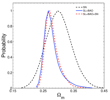
Figure 1: Constraints on $\Lambda$CDM model. The blue curve is the result from SL+BAO, the black one is from SN, and the the red one is from SL+BAO+SN.

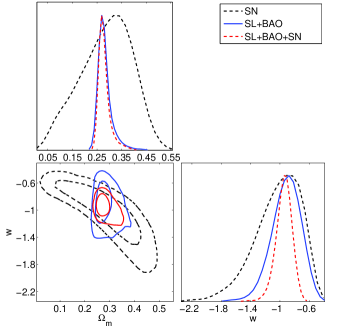
Figure 2: Constraints on XCDM model. The blue curve is the result from SL+BAO, the black one is from SN, and the the red one is from SL+BAO+SN.

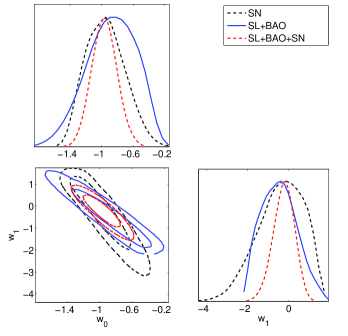
Figure 3: Constraints on CPL parameterization with fixed $\Omega_{m}=0.315$. The blue curve is the result from SL+BAO, the black one is from SN, and the the red one is from SL+BAO+SN.

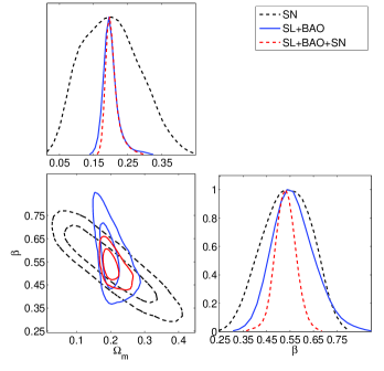
Figure 4: Constraints on RDE model. The blue curve is the result from SL+BAO, the black one is from SN, and the the red one is from SL+BAO+SN.

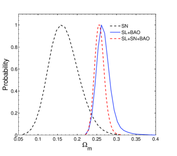
Figure 5: Constraints on DGP. The blue curve is the result from SL+BAO, the black one is from SN, and the the red one is from SL+BAO+SN.

3.2 Dark energy with constant equation of state

In this case, dark energy is described by a hydrodynamical energy-momentum tensor with constant equation of state coefficient $w=p/{\rho}$, which leads to cosmic acceleration whenever $w<-1/3$ (Ratra et al., 1988).

For standard rulers, standard candles and the combined analysis, confidence regions (corresponding to 68.3% and 95.8% confidence levels) in the ($\Omega_{m}$, w) plane are shown in Fig. 2, with the best-fit parameters: $\left\{\Omega_{m},w\right\}=\left\{0.282^{+0.021}_{-0.023},-0.917^{+0.194}_{-0.188}\right\}$, $\left\{\Omega_{m},w\right\}=\left\{0.287^{+0.104}_{-0.111},-0.917^{+0.308}_{-0.304}\right\}$, and $\left\{\Omega_{m},w\right\}=\left\{0.280^{+0.018}_{-0.019},-0.947^{+0.102}_{-0.094}\right\}$ from SL+BAO, SN, and SL+BAO+SN, respectively. As can be seen from Fig. 2, standard rulers (SL+BAO) and standard candles (SN) have different degeneracies in the parameter space. Consequently, their restrictive power is different. This fact makes the joint constraint more restrictive. Our results are in perfect agreement with the previous results obtained from the ESSENCE supernova survey team (Wood-Vasey et al., 2007) who obtained $\left\{\Omega_{m},w\right\}=\left\{0.274^{+0.033}_{-0.020},-1.07\pm{+0.09}\pm{-0.12}\right\}$ and the Union1 SNIa compilation (Kowalski et al., 2008) whose results were following: $\left\{\Omega_{m},w\right\}=\left\{0.274^{+0.033}_{-0.020},-0.969^{+0.059}_{-0.063}{{}^{+0.063}_{-0.066}}\right\}$.

3.3 Chevalier-Polarski-Linder (CPL) model

Constant cosmic equation of state of the XCDM cosmology is only a phenomenological description, which cannot be ultimately true. Being fundamentally different from the cosmological constant, it must have some dynamical reason e.g. in a scalar field settling down on the attractor. Therefore one should expect that such scalar field was evolving and left the trace of its evolution on the equation of state. So, it would be natural to expect that the $w$ coefficient varied in time, i.e. $w=w(z)$. In this paper, we take a Taylor expansion of $w(z)$ with respect to the scale factor, which leads to the following redshift dependence: $w(z)=w_{0}+w_{1}\frac{z}{1+z}$. This is so called Chevalier-Polarski-Linder (CPL) model proposed in (Chevalier & Polarski, 2001; Linder, 2004).

It has been known for some time that it is hard to get good and stringent fits for all parameters in this model. Hence, we fix matter density parameter at the best-fit value $\Omega_{m}=0.315$ based on the recent Planck observations (Ade et al., 2014). Our best fit values for the CPL model parameters are $\left\{w_{0},w_{1}\right\}=\left\{-0.879^{+0.414}_{-0.431},-0.463^{+2.108}_{-1.717}\right\}$, $\left\{w_{0},w_{1}\right\}=\left\{-0.951^{+0.249}_{-0.247},-0.4034^{+1.160}_{-1.139}\right\}$, and $\left\{w_{0},w_{1}\right\}=\left\{-0.965^{+0.154}_{-0.155},-0.241^{+0.498}_{-0.501}\right\}$ from SL+BAO, SN, and SL+BAO+SN, respectively. Confidence regions (corresponding to 68.3% and 95.8% confidence levels) for standard rulers, standard candles and the combined analysis in the ($w_{0}$, $w_{1}$) plane are shown in Fig. 3. One can notice that confidence contours from standard rulers and standard candles are inclined with respect to each other. This is a promising signal in light of the colinearity of $w_{0}$ and $w_{1}$ parameters (due to their fundamental anticorrelation), which has so far been a major obstruction in getting stronger constraint on them. Such inclination gives us hope that combined analysis will eventually lead to more precise assessment of $w_{0}$ and $w_{1}$ and decide whether cosmic equation of state evolved or not.

The results obtained with standard rulers turned out to correspond well with previous work by Biesiada et al. (2011), whose results (for standard rulers) were $w_{0}=-0.993\pm 0.207,w_{1}=0.609\pm 1.071$. As far as standard candles are concerned, the result of joint analysis from WMAP+BAO+$H_{0}$+SN given by Komatsu et al (2011) is $w_{0}=-0.93\pm 0.13,w_{1}=0.41^{+0.72}_{-0.71}$. Moreover, the combined analysis of standard rulers and candles performed in Biesiada et al. (2011) resulted in the following best fits: $w_{0}=-0.989\pm 0.124,w_{1}=0.082\pm 0.621$. These results are in agreement with ours within $1\sigma$. In addition, our joint analysis tends to support the models with a varying equation of state which are very close to the $\Lambda$CDM model ($w_{0}=-1$, $w_{1}=0$).

3.4 Ricci Dark Energy model

There are other cosmological models that have gained a lot attention, one of them is the so called holographic dark energy, which is inspired by the holographic principle resulting from quantum gravity. It is well known that gravitational entropy of a given closed system with a characteristic length scale $L$ is not proportional to its volume $L^{3}$, but to its surface area $L^{2}$ (Bekenstein, 1981; Gao et al., 2009). Because the cosmological constant $\Lambda$ scales like inverse length squared, one could postulate this length scale coinciding with present Hubble horizon. This way the coincidence and fine tuning problem could be alleviated. However it turned out that such model has troubles with explaining accelerated expansion of the Universe. Therefore Gao et al. (2009) proposed to choose $|R|^{-1/2}$ as the infrared cutoff, where $R=-6(\dot{H}+2H^{2})$ is Ricci scalar. In this section we will confront this model with standard rulers and standard candles data. The density of dark energy in this model is

$${\rho_{de}}={3{\beta}M^{2}_{Pl}(\dot{H}+2H^{2})}$$ (18)

where $\beta>0$ is some constant parameter to be fitted.

With the methods described above, we obtain the following best fits for RDE model: $\left\{\Omega_{m},\beta\right\}=\left\{0.201^{+0.017}_{-0.019},0.566^{+0.087}_{-0.086}\right\}$, $\left\{\Omega_{m},\beta\right\}=\left\{0.202^{+0.086}_{-0.088},0.534^{+0.104}_{-0.105}\right\}$, and $\left\{\Omega_{m},\beta\right\}=\left\{0.201^{+0.016}_{-0.016},0.531^{+0.041}_{-0.041}\right\}$ from SL+BAO, SN, and SL+BAO+SN, respectively. These results are also illustrated in Fig. 4. These results are in agreement with previous work of Cao, Covone & Zhu (2012). Additionally the best fits for different probes are very close to each other.

3.5 Dvali-Gabadadze-Porrati model

Cosmological models we investigated so far were based on the Einstein’s theory of gravity. There are also other approaches which seek an explanation of accelerated expansion of the Universe in modifications of General Relativity. Dvali-Gabadadze-Porrati (DGP) brane world model is a well-known example of this class, based on the assumption that our 4-dimensional spacetime is embedded into a higher dimensional bulk spacetime (Dvali & Poratti, 2000).

In this model, the Friedman equation is modified to

$${H^{2}+\frac{k}{a^{2}}}={\left[\sqrt{\frac{\rho}{3M^{2}_{Pl}}+\frac{1}{4r_{c}}}+\frac{1}{2r_{c}}\right]^{2}}$$ (19)

where $M_{Pl}=\sqrt{\frac{\hbar c}{8\pi G}}$ is the (reduced) Planck mass, $r_{c}=\frac{M_{Pl}^{2}}{2M_{5}^{2}}$ (with $M_{5}$ denoting 5-dimensional reduced Planck mass) is the crossover scale. Introducing the omega parameter: $\Omega_{rc}=1/(4r^{2}_{c}H^{2}_{0})$, one can rewrite the Eq. (19) in the form leading to the Hubble function given in Table 1 (assuming also flat Universe). Friedman equation leads also to the normalization condition: $\Omega_{k}+(\sqrt{\Omega_{r_{c}}}+\sqrt{\Omega_{m}+\Omega_{r_{c}}})^{2}=1$, which simplifies to $\Omega_{r_{c}}=\frac{1}{4}(1-\Omega_{m})^{2}$ under assumption of flat Universe. Therefore, the flat DGP model contains only one free parameter, $\Omega_{m}$. The best fit values for the mass density parameter in DGP model obtained from SL+BAO, SN, and SL+BAO+SN are: ${\Omega_{m}}=0.269^{+0.014}_{-0.016}$, ${\Omega_{m}}=0.165^{+0.036}_{-0.035}$, and ${\Omega_{m}}=0.257^{+0.011}_{-0.012}$, respectively. These results are also illustrated in Fig. 5.

Former work done by Xu & Wang (2010) indicated ${\Omega_{m}}=0.266^{+0.0298}_{-0.0304}$ and the results of Biesiada et al. (2011) ${\Omega_{m}}=0.267\pm 0.013$ from CMB+BAO+SL+SN match accurately with our results. Moreover, our results are in a very good agreement with Cao, Covone & Zhu (2012).

Closing this section, let us stress that we have not only constrained cosmological models, but also we considered the evolution of slope factor in the mass density profile of lensing galaxies. In consequence, we also obtained the best fits for $\gamma$ parameters, as shown in Table 1. One can see, that the $\gamma$ parameters estimated in different cosmological models are very similar. It suggests that the method of using distance ratios from strong lensing systems can be effective in cosmological applications. More precisely, since the $\gamma$ parameters of lens mass distribution model seem to be unaffected by cosmological model assumed, one can hope to calibrate them within say $\Lambda$CDM model and then use the best fits as an input for cosmological model testing with the samples like ours (118 lenses) or similar ones obtained in the future.

4 Model selection

In the previous section, we obtained the best fits for five cosmological models from 118 galactic-scale strong lensing systems combined with 6 BAO observations. However, the $\chi^{2}$ statistic alone does not provide any way to compare the competing models and decide which one is preferred by the data. This question can be answered with model selection techniques (Cao, Zhu & Zhao, 2012).

Therefore, we used of two criteria: Akaike Criterion (AIC) (Akaike, 1974) and Bayesian Information Criterion (BIC) (Schwarz, 1978). They have became standard in applied statistics, were first used in cosmology by Liddle (2004) and then e.g. by Godłowski & Szydłowski (2005) or Biesiada (2009). The value of AIC – approximately unbiased estimator of the Kullback-Leibler divergence between the given model and the “true” one can be calculated as

$$AIC=-2lnL_{max}+2k$$ (20)

where $L_{max}$ is the maximum likelihood value, $k$ is the number of free parameters in the model. In our case $k$ comprises both cosmological parameters and galaxy mass density slopes. If the uncertainties are Gaussian likelihood can be calculated from the chi-square function $\chi^{2}=-2lnL_{max}$. The value of $AIC$ for a single model is meaningless. What is useful is the difference in AIC between cosmological models $\Delta AIC$. This difference is usually calculated with respect to the model which has the smallest value of AIC

$$\Delta AIC(i)=AIC(i)-AIC_{min}$$ (21)

where the index $i=1,...,5$ represents cosmological models and $AIC_{min}=min\left\{AIC(i)\right\}$. BIC is defined in a very similar manner to AIC, but it adds the information about the sample size $N$:

$$BIC={\chi^{2}}+2klnN$$ (22)

For the purpose of model selection we only used the standard rulers, i.e. BAO combined with 118 lensing data. Table 3 lists the AIC and BIC difference of each model. One can see that both $AIC$ and $BIC$ criteria support $\Lambda$CDM as the best cosmological model, in the light of current observational strong lensing data. Concerning the ranking of other competing models, AIC and BIC criteria give different conclusions. According to the AIC, next are the RDE and XCDM model: odds against them with respect to $\Lambda$CDM (see (Biesiada, 2009) for details) are 2.6:1 (they differ at the second decimal place). Then the CPL and DGP are slightly worse supported, with odds against 2.8:1. In summary, one can say that besides the $\Lambda$CDM as the best one, all other models get similar support by standard rulers. On the other hand BIC criterion gives a different ranking: next after $\Lambda$CDM is the DGP brane model with odds against equal to 2.8:1. Then there are RDE (odds against 10.1 : 1) and XCDM (odds against 10.5:1) while CPL model gets the smallest support with odds against 11.5:1. In summary, one can state that BIC substantially penalizes cosmological models with more than one free parameter. In particular our findings are in contrast with (Biesiada, 2009) who claimed that DGP model is strongly disfavored by the data.

Table 3: Summary of the information criteria, AIC and BIC for the combined SL+BAO data.

Model	AIC	$\Delta$AIC	BIC	$\Delta$BIC
$\Lambda$CDM	320.71	0	323.53	0
XCDM	322.61	1.89	328.25	4.71
CPL	322.77	2.06	328.41	4.88
RDE	322.59	1.88	328.23	4.63
DGP	322.76	2.05	325.58	2.05

5 Summary and Conclusion

In this paper, we used standard rulers and standard candles (separately and jointly) to explore five popular dark energy models under assumption of spatial flatness of the Universe. As standard rulers, we used new galactic-scale strong lensing data set compiled by Cao et al. (2015a) combined with BAO diagnostics. Supernovae Ia served as standard candles. In order to compare the degree of support given by the standard rulers to various competing dark energy models, we performed a model selection using the AIC and BIC information criteria.

The main conclusions of this paper can be summarized as follows. Firstly, relaxing the mass density profile of SIS model to a more general power-law density profile, the best fitted $\gamma$ parameters are in agreements with each other irrespective of the cosmological model considered. This demonstrates that inclusion of mass density power index as a free parameter does not lead to noticeable spurious effects of mixing them with cosmological parameters in statistical procedure of fitting. Therefore, we can say that galactic strong lensing systems may provide a complementary probe to test the properties of dark energy. Secondly, because standard rulers and standard candles have different parameter degeneracies in cosmology, joint analysis of standard rulers and standard candles gives much more restrictive results for cosmological parameters. Thirdly, the information theoretic criteria (AIC and BIC) support the claim, that cosmological constant model is still the best one and there is no reason to prefer any more complex model. In light of forthcoming new generation of sky surveys like the EUCLID mission, Pan-STARRS, LSST, JDEM, which are estimated to discover from thousands to tens of thousands of strong lensing systems it would be interesting to stay tuned and look forward to seeing whether this conclusion could be changed by more gravitational lensing systems observed in the future.