Simultaneous observation of water and class I methanol masers toward class II methanol maser sources

Abstract

We present a simultaneous single-dish survey of 22 GHz water maser and 44 GHz and 95 GHz class I methanol masers toward 77 6.7 GHz class II methanol maser sources, which were selected from the Arecibo methanol maser Galactic plane survey (AMGPS) catalog. Water maser emission is detected in 39 (51 %) sources, of which 15 are new detections. Methanol maser emission at 44 GHz and 95 GHz is found in 25 (32 %) and 19 (25 %) sources, of which 21 and 13 sources are newly detected, respectively. We find 4 high-velocity ($>$30  km s^-1) water maser sources, including 3 dominant blue- or redshifted outflows. The 95 GHz masers always appear with the 44 GHz maser emission. They are strongly correlated with 44 GHz masers in velocity, flux density, and luminosity, while they are not correlated with either water or 6.7 GHz class II methanol masers. The average peak flux density ratio of 95 GHz to 44 GHz masers is close to unity, which is two times higher than previous estimates. The flux densities of class I methanol masers are more closely correlated with the associated BGPS core mass than those of water or class II methanol masers. Using the large velocity gradient (LVG) model and assuming unsaturated class I methanol maser emission, we derive the fractional abundance of methanol to be in a range of $4.2\times 10^{-8}$ to $2.3\times 10^{-6}$, with a median value of $3.3\pm 2.7\times 10^{-7}$.

1 Introduction

Masers are widely recognized as indirect tools for understanding the early stages of massive star formation. Water masers are frequently detected in star-forming regions. They are pumped by collisions with neutral particles and appear in accretion disks or outflows (Elitzur et al., 1989; Torrelles et al., 1997; Moscadelli et al., 2006). Furthermore, water masers are detected near young stellar objects (YSOs) regardless of mass, and more massive YSOs tend to have stronger maser emission (Genzel & Downes, 1977; Furuya et al., 2003; Bae et al., 2011). Water masers often exhibit significant variability in velocity and flux density (Rodriguez et al., 1980; Bae et al., 2011; Choi et al., 2012), and sometimes high-velocity features near outflows (Gwinn et al., 1992; Gwinn, 1994). Beuther et al. (2002) investigated the spatial relationship between water and 6.7 GHz methanol masers. Both maser species are closely associated with the early stages of massive star formation, but no spatial correlation was observed.

Many methanol maser transitions show maser activity. These maser transitions are empirically divided into two groups: class I and class II (Menten, 1991). Class I methanol masers such as the $4_{-1}-3_{0}~{}E$, $7_{0}-6_{1}~{}A^{+}$, $5_{-1}-4_{0}~{}E$, and $8_{0}-7_{1}~{}A^{+}$ lines at 36, 44, 84, and 95 GHz, respectively, are normally detected offset from HII regions, infrared sources, OH, and H₂O masers (Plambeck & Menten, 1990; Kurtz et al., 2004). However, class II methanol masers such as the $5_{1}-6_{0}~{}A^{+}$, $2_{0}-3_{-1}~{}E$, $9_{2}-10_{1}~{}A^{+}$, and $J_{0}-J_{-1}~{}E$ lines at 6.7, 12, 23, and 157 GHz, respectively, are found close to other star formation indicators (Walsh et al., 1998). Using a theoretical model, Cragg et al. (1992) inferred that class I methanol masers are pumped by collisions, while class II masers are excited by radiative pumping.

Methanol masers are primarily found in massive star-forming regions (Minier et al., 2003; Breen et al., 2013), although weak class I methanol masers are detected in several low- and intermediate-mass star forming regions as well (Kalenskii et al., 2010; Bae et al., 2011). Class I methanol masers usually appear in the interface between outflows and the surrounding regions (Plambeck & Wright, 1988; Plambeck & Menten, 1990; Kurtz et al., 2004; Cyganowski et al., 2009; Voronkov et al., 2006, 2014). Val’tts et al. (2000) reported that the peak flux density of 44 GHz masers is on average about three times higher than that of the associated 95 GHz class I methanol maser. Class II methanol masers, on the other hand, are detected at an early age evolutionary phase of massive star formation. There is ongoing debate about whether class II masers trace accretion disks or outflows (Norris et al., 1993; Pestalozzi et al., 2004; Walsh et al., 1998; Minier et al., 2000; Dodson et al., 2004).

Slysh et al. (1994) surveyed 44 GHz class I methanol maser emission with 5 to 10 Jy detection limits (3$\sigma$) toward about 250 HII regions and water and 6.7 GHz class II methanol maser sources. Of the 55 detected 44 GHz maser sources, 64 % are related to 6.7 GHz masers. They suggested that class I and class II masers have anti-correlations of velocity and flux density. However, their observations were based on single-dish data with no accurate positions and made towards a source sample with significant selection biases. Ellingsen (2005) searched for similar anti-correlations between 95 GHz class I and 6.7 GHz masers, but did not find any anti-correlation, either in velocity or flux density.

In this study, we report a simultaneous survey of 22 GHz water and 44 GHz and 95 GHz class I methanol masers toward 6.7 GHz class II methanol masers, which were selected from the Arecibo methanol maser Galactic plane survey (AMGPS) catalog (Pandian et al., 2007). The AMGPS covered the inner Galactic region of $35.2\arcdeg\lesssim l\lesssim 53.7\arcdeg$ and $|b|\lesssim 0.41\arcdeg$ with a detection limit of 0.27 Jy (3$\sigma$). The properties of the AMGPS sources such as distance, luminosity, and kinetic temperature have been subsequently studied by Pandian et al. (2009, 2011, 2012). The AMGPS sources may represent various evolutionary stages of massive star formation, because they were identified by a very sensitive unbiased survey. We statistically investigate the detection rates of the observed maser species and correlations between them. We are particularly interested in the relationship between class I and II methanol masers. Since water and class I methanol masers are both pumped by collision mechanisms, one may expect a significant correlation between them. Chen et al. (2012) recently suggested selection criteria for the Bolocam Galactic Plane Survey (BGPS) clumps likely to have an associated 95 GHz class I methanol maser. We also examine the validity of these criteria using our data sets.

Section 2 gives the source selection and observation methodology. Section 3 presents the detection statistics, new detections, and short descriptions of some interesting sources. Section 4 describes velocity characteristics, flux densities and luminosities, comparison with the BGPS clump parameters, and methanol column densities and abundances. Section 5 summarizes the main results.

2 Source Selection and Observations

2.1 Source Selection

We selected 77 sources from the AMGPS catalog of 88 6.7 GHz methanol maser sources. The catalog originally consisted of 86 sources (Pandian et al., 2007), and later 2 new sources (G37.04-0.04 and G49.42+0.32) were added via MERLIN observations (Pandian et al., 2011). Considering the beam size of the telescope at 95 GHz, 33$\arcsec$ (see § 2.2), we excluded 9 sources in two very crowded regions: W49N (G43.15+0.02, G43.16+0.02, G43.17+0.01, G43.17-0.00, and G43.18-0.01) and W51 (G49.47-0.37, G49.48-0.40, G49.49-0.37, and G49.49-0.39). We also rejected G49.42+0.32 due to its proximity to G49.41+0.33 (Pandian et al., 2011), and G41.87-0.10 due to its uncertain coordinates (Pandian et al., 2007). The systemic velocities of the individual sources were taken from the previous molecular line observations (Pandian et al., 2009, 2012). Table Simultaneous observation of water and class I methanol masers toward class II methanol maser sources lists the 77 sources in our sample together with their equatorial coordinates and systemic velocities.

2.2 Observations

Using the Korean VLBI Network (KVN) 21 m telescopes, we performed simultaneous surveys of the H₂O  $6_{16}-5_{23}$ (22.23508 GHz), CH₃OH  $7_{0}-6_{1}A^{+}$ (44.06943 GHz), and CH₃OH  $8_{0}-7_{1}A^{+}$ (95.169463 GHz) masers toward the 77 class II methanol maser sources. The KVN consists of three 21 m telescopes (Kim et al., 2011; Lee et al., 2011). Each telescope is equipped with a multi-frequency receiving system with 22 GHz, 44 GHz, 86 GHz, and 129 GHz bands (Han et al., 2008). Two telescopes at the Yonsei and Ulsan sites were used in single-dish mode. Table 2 presents the aperture efficiencies, half-power beam widths (HPBWs), and conversion factors of the telescopes. All spectra were obtained by position switching. For calibration, we adopted the standard chopper-wheel method, and the line intensity was observed on the $T^{*}_{\rm A}$ scale. The pointing and focus were checked every 2$-$3 hours. The system temperature (T_sys) ranges were 70$-$90 K at 22 GHz, 100$-$150 K at 44 GHz, and 150$-$250 K at 95 GHz. The aperture efficiencies of the used telescopes remain constant within 15% for elevations of $\geq$20$\arcdeg$ at the observing frequencies (Lee et al., 2011). The bandwidths were set to 32 MHz with 4096 channels. The KVN receiving systems support dual-polarization mode, and the computational backend can process up to four inputs simultaneously (Lee et al., 2011). To approximately equalize root-mean-square ($rms$) noise levels in different bands, we observed a single polarization for the 22 GHz and 44 GHz bands and dual polarization for the 95 GHz band. The resultant noise levels were about 1.5 Jy (3$\sigma$) at a velocity resolution of 0.2  km s^-1 for all three bands. The KVN telescopes are shaped Cassegrain and hence have fairly high first side lobe levels of about 5 % (Kim et al., 2011; Lee et al., 2011). We made 7$\times$7 grid maps with half-beam spacing for all detected 22 and 44  GHz maser sources in order to assess if the maser emission is contaminated by any nearby strong source. Here 95  GHz maser sources were excluded because they all correspond to 44  GHz maser sources (see § 3.1). The observation took a total of 18 days to complete and were undertaken between 2011 Nov – 2012 Mar: 15 days for the survey and 3 days for the grid mapping.

We also observed 4 sources in the ¹³CO (J=1$-$0) (110.201353 GHz) line and one of them in the HCO⁺ (J=1$-$0) (89.188523 GHz) line using the Taeduk Radio Astronomy Observatory (TRAO) 14 m telescope on 2014 March 17. The aim of these observations was to investigate the origin of the water maser features with large velocity offsets (see § 3.3.6). The system temperatures were 560 K at 89 GHz and 760 K at 110 GHz. The main-beam efficiencies of the telescope are 50% and 49% at 89 GHz and 110 GHz, respectively. All the data were reduced and analyzed with the GILDAS/CLASS package and IDL. The bisector method was adopted for the linear regression calculations (Isobe et al., 1990).

3 Results

3.1 Detection Rates

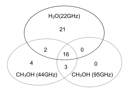
Figure 1: Venn diagram displaying the number of sources detected in the three observed maser transitions.

Table Simultaneous observation of water and class I methanol masers toward class II methanol maser sources summarizes the observational results, and Figure 1 displays the statistics of detected maser sources. We detected at least one maser species in 46 of the 77 sources. Water masers were detected in 39 (51 %) sources. 44 GHz and 95 GHz methanol masers were detected in 25 (32 %) and 19 (25 %) sources, respectively. Interestingly, 95 GHz masers always accompany 44 GHz maser emission and often (84 %) appear with water maser emission. 44 GHz masers also mostly (72 %) accompany water maser emission.

The 6.7 GHz maser sources in our sample have a wide range of peak flux densities, 0.1–55.6 Jy, and isotropic maser luminosities, $\rm 10^{-9}-10^{-5}\,L_{\sun}$ (Pandian et al., 2007, 2009). We investigate the detection rates of the three observed maser transitions along with the flux density and luminosity of the 6.7 GHz maser emission (Figure 8). All three rates tend to increase with the flux density and luminosity, although the trend is not strong. Ellingsen (2005) also surveyed 95 GHz maser emissions with a flux limit of $\sim$4 Jy (3$\sigma$) toward sixty six 6.7 GHz methanol maser sources, which had been found by previous blind surveys, and detected emission in 25 sources. The detection rate (38%) is significantly higher than our value (25 %) in spite of considerably poorer sensitivity. This is presumably because their sample contains more bright sources than our sample. The fraction of sources with flux densities of $\geq$10 Jy is about 60% for their sample but about 20% for ours. We examine the detection rate of 44 GHz class I methanol maser emission for sources with strong water maser emission, and find that the rate is 89% (8/9) for the sources with peak flux densities of water maser emission $>$ 20 Jy. Meanwhile the rate is much lower (33%, 10/30) for the sources with flux densities $<$20Jy. We also find a similar trend for the detection rate of water maser emission. The rate is 100% (4/4) for the sources with flux densities of 44 GHz methanol maser emission $>$10 Jy while it is 67% for the others.

3.2 New Maser Sources

We identify 15 of the 39 water maser detections as new discoveries using the VizieR service (Ochsenbein et al., 2000) by comparing our results with previous surveys: Palagi et al. (1993); Codella et al. (1994); Han et al. (1998); Forster & Caswell (1999); Valdettaro et al. (2001); Codella et al. (2004); Szymczak et al. (2005); Urquhart et al. (2011). Szymczak et al. (2005) also searched for water maser emission toward 4 sources in our sample (G36.70+0.09, G37.02-0.03, G37.04-0.04, G38.03-0.30), but did not detect emission in any of these sources. They used the Effelsberg 100 m telescope (HPBW $\simeq$ 40$\arcsec$) with a flux limit of 1.5 Jy (3$\sigma$). The observed positions are offset from our 6.7 GHz maser positions by 27$\arcsec$–87$\arcsec$. Thus their nondetection may be due both to slightly different observed positions and relatively small beam size. We can apply the same explanation for two other sources (G40.28-0.22 and G42.03+0.19) in which no water maser emission was detected by Urquhart et al. (2011) using the GBT 100 m telescope with a flux limit of 0.4 Jy (3$\sigma$).

Meanwhile, there have been many fewer surveys of class I methanol masers. We find that 21 of the 25 detected 44 GHz methanol maser sources are new detections (Kurtz et al., 2004; Cyganowski et al., 2009; Bayandina et al., 2012). Thirteen of the 19 detected 95 GHz methanol maser sources appear to be new detections from a comparison with the catalogues of Chen et al. (2011, 2012), who also used single-dish telescopes. Among the new sources, G37.55+0.19 and G45.49+0.13 have been observed by Chen et al. (2011) with the Mopra 22 m telescope (HPBW $\simeq$ 36$\arcsec$) at a detection limit of 1.6 Jy (3$\sigma$). Their positions are different from ours by 33$\arcsec$ –41$\arcsec$.

3.3 Notes on Selected Sources

3.3.1 G35.03+0.35, G43.04-0.46, and G45.07+0.13

These three are the only already-known sources both with water and 44 GHz class I methanol masers in our sample. We confirm that the water masers vary substantially in both the velocity and flux density of their emission, while the 44 GHz masers do not. Forster & Caswell (1999) observed water maser emission of 18.5 Jy at 68.5 km s^-1 in G35.03+0.35. This is very different from our result, 62.5$\pm$0.9 Jy at 44.7 km s^-1. Cyganowski et al. (2009) detected 44 GHz maser emission at 52.8 km s^-1 using the Very Large Array (VLA). The peak velocity is consistent with our value, 52.8 km s^-1. For G43.04-0.46, Valdettaro et al. (2001) observed water maser emission of 5.1 Jy at 57.55 km s^-1, which is very different from our measurement, 5.6$\pm$0.7 Jy at 45.7 km s^-1. Kurtz et al. (2004) observed 44 GHz maser emission of 3.8 Jy at 58.0 km s^-1 with the VLA. We also detected the maser emission of 8.7$\pm$1.1 Jy at the same velocity. There have been several reports of water maser detection in G45.07+0.13. The peak flux densities and velocities are 50.7 Jy at 60.1 km s^-1, 21.5 Jy at 60.6 km s^-1, 41 Jy at 60.1 km s^-1, and 23.2$\pm$0.6 Jy at 60.1 km s^-1 by Palagi et al. (1993), Forster & Caswell (1999), Valdettaro et al. (2001), and this study, respectively. Kurtz et al. (2004) showed 44 GHz maser emission of 1.1 Jy at 59.3 km s^-1 and we also detected a peak flux density of 1.7$\pm$0.5 Jy at 59.2 km s^-1.

3.3.2 G36.92+0.48, G38.26-0.08, G41.58+0.04, G43.80-0.13, G44.64-0.52, and G45.07+0.13

The systemic velocities of these sources were not determined by the NH₃ lines (Pandian et al., 2012) but by the ¹³CO ($J$ = 2$-$1) or CS ($J$ = 5$-$4) lines (Pandian et al., 2009). G43.80-0.13 and G45.07+0.13 show strong NH₃ lines, but the line profiles are complicated (Pandian et al., 2012). These two sources have all three maser species, and G43.80-0.13 is the strongest water maser source in our sample (Table 3). The other four sources have no detectable NH₃ line emission. Only G38.26-0.08 among them shows water maser emission.

3.3.3 G37.02-0.03 and G37.04-0.04

These two sources are separated by 47″.7 and overlap within the HPBW of the telescope at 22 GHz. They exhibit two common water maser lines at 80.7 and 81.6  km s^-1. Therefore, we count them as one detection. A more detailed investigation using interferometric observations is required to clarify the origin of water maser emission in this area. The BGPS counterpart, G037.042-00.034, is closer to G37.04-0.04 than G37.02-0.03.

3.3.4 G38.66+0.08, G39.39-0.14, and G42.43-0.26

These sources are associated with ultracompact (UC) HII regions (Pandian et al., 2010). G42.43-0.26 has all three maser species, while G39.39-0.14 shows only class I methanol masers, and G38.66+0.08 does not display any maser emission.

3.3.5 G40.28-0.22 and G48.99-0.30

G40.28-0.22 and G48.99-0.30 are the strongest 44 GHz and 95 GHz maser sources in our sample, respectively (Table 3). G40.28-0.22 has a peak flux density of 89.2$\pm$1.4 Jy at 44 GHz  and 72.7$\pm$1.0 Jy at 95 GHz. This object is associated with a luminous ($L_{\rm bol}$$\simeq$2.1$\times$10⁵ $L_{\sun}$) YSO, which might be a hypercompact HII region (Pandian et al., 2010). Water and 44 GHz methanol masers were newly detected, while 95 GHz methanol maser emission has been detected by Chen et al. (2011) with a peak flux density of 53.2 Jy at 72.8 km s^-1. Urquhart et al. (2011) searched for water maser emission at this site, but did not detect any. G48.99-0.30 has a 44 GHz peak flux density of 93.2$\pm$1.2 Jy at 66.4 km s^-1  and a 95 GHz peak flux density of 54.2$\pm$0.9 Jy at 66.5 km s^-1. Both class I methanol maser transitions are new detections, whereas the water maser emission has been detected by multiple surveys (see Table 1). For instance, Codella et al. (1994) and Valdettaro et al. (2001) observed water maser emission of 7 Jy at 71.0 km s^-1 and 8 Jy at 70.9 km s^-1, respectively. Urquhart et al. (2011) detected a peak flux density of 58.9 Jy at 65.3 km s^-1, which is similar to our detection, 62.4$\pm$0.8 Jy at 66.0 km s^-1.

3.3.6 High velocity Features of Water Maser

We found 4 water maser sources showing very different ($>$30  km s^-1) velocity components from the systemic velocities. G35.59+0.06, G37.60+0.42, G41.08-0.13, and G41.34-0.14 have maser lines with velocity offsets of $-$60.5, +48.0, $-$77.6, and +47.5  km s^-1  respectively. Breen et al. (2010) also found 10 water maser sources with large ($>$30  km s^-1) relative velocity components with respect to 6.7 GHz methanol maser emission. The fraction of their sources in their sample (approximately 200 sources) which show high velocity emission (5%) is half that of this study (4/39, 10%). These features can be produced by high-velocity jets/outflows from the massive YSOs associated with 6.7 GHz methanol masers (Gwinn et al., 1992; Gwinn, 1994) or associated with other YSOs at different distances along the same line of sight. In order to distinguish between the two possibilities, we observed ¹³CO (J=1$-$0) line emission toward these sources, and found no ¹³CO line emission related to the large velocity-offset features in any of them except G41.34$-$0.14 (Figure 7). We also observed G41.34$-$0.14 in the HCO⁺ (J=1$-$0) line, which is a very reliable tracer of massive star-forming cores (e.g., Purcell et al. 2006), and detected line emission only at the systemic velocity. Therefore, the large velocity-offset features are likely to be high-velocity components caused by jets/outflows, even though we cannot exclude the possibility that the feature of G41.34$-$0.14 may be associated with a low-mass YSO at a different distance in the same line of sight.

G37.60+0.42 has a maser emission near the systemic velocity as well, while the others do not. G35.59+0.06 and G41.08$-$0.13 are so-called dominant blue-shifted water maser outflows. Caswell & Phillips (2008) reported three such water maser sources and suggested that they can be generated from pole-on jets. G41.34$-$0.14 may be the red-shifted counterpart of the dominant blue-shifted water maser sources. Follow-up observations with higher resolution are required to understand the origin of these objects.

4 Analyses

4.1 Velocity Characteristics

Figure 9 shows the distribution of the peak velocity offsets from the systemic velocities for the four maser species. The bin size is 2  km s^-1. The average offsets of the 6.7 GHz, 22 GHz, 44 GHz, and 95 GHz masers are $-$0.0$\pm$5.0, $-$0.6$\pm$4.8, 0.2$\pm$1.1, and 0.4$\pm$1.1 km s^-1, respectively. In these calculations, the four high-velocity water maser sources have been excluded. The velocity offsets of the 44 GHz and 95 GHz masers are always within $\pm$4  km s^-1. This is consistent with the findings of previous studies (e.g., Fontani et al. 2010; Bae et al. 2011). Plambeck & Menten (1990) and Kurtz et al. (2004) suggest that the class I methanol maser emission is associated with ambient molecular cloud that is heated by outflows and is not accelerated by the outflow. Our results support this hypothesis. The offsets of 6.7 GHz class II methanol masers are much more widely distributed, but are still within $\pm$10  km s^-1 for 95% of the sources. The distribution is double peaked with a dip around zero. This is consistent with the finding of Byun et al. (2012) for a large sample of 284 6.7 GHz maser sources. In contrast, the distributions are single peaked around zero for the other masers. The offset dispersion of water maser lines appears to lie between those of class I and class II methanol masers. Half of the sources are within $\pm$2.3  km s^-1 and $\pm$3.7  km s^-1 for water and 6.7 GHz masers, respectively. For comparison, Fontani et al. (2010) surveyed 6.7 GHz, 44 GHz, and 95 GHz methanol masers toward 296 massive YSO candidates, which had been observed in water maser emission. They found that water and class II methanol masers have very similar single-peaked distributions of velocity offsets. The bin size in their histograms was 6  km s^-1. This large bin size may have impacted their ability to identify a double-peaked distribution of 6.7 GHz masers. When we use the same bin size, the distribution of 6.7 GHz masers in our sample is also changed to be single peaked. Further detailed studies are required to clarify the statistical significance and physical implications of the dip observed in this study. Almost all of the class I maser sources in their sample showed velocity offsets within $\pm$6 km s^-1.

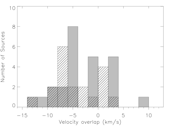
Figure 11: Histogram of the velocity overlap between class I and 6.7 GHz class II methanol masers. Filled and slant bars indicate 44 GHz and 95 GHz masers, respectively. A negative value means that the velocity ranges of the two masers overlap (See the text for details).

Figure 10 compares the velocity offsets of class I and class II masers. Large velocity offsets of both masers appear to be avoided. Slysh et al. (1994) reported that class I and class II are anti-correlated in the velocities where they exhibit strong emission. Some of our data show the anti-correlation, but almost do not follow the trend. We derive the velocity overlap of class I and class II methanol maser spectra to examine the relationship between the two classes. The velocity overlap is defined by the difference between the lowest velocity of the class with higher mean velocity and the highest velocity of the other class with lower mean velocity (Ellingsen, 2005). Negative values of velocity overlap hence imply that the velocity ranges of the two classes overlap. Figure 11 displays a histogram of the velocity overlap. Nineteen (76%) of twenty-five 44 GHz maser sources and fourteen (74%) of nineteen 95 GHz maser sources show negative values. This portion is slightly higher than that of Ellingsen (2005) for 95 GHz maser sources, 62% (23/37).

4.2 Flux Densities and Luminosities

Tables 3 and 4 present the peak flux densities and the isotropic luminosities of the detected masers, respectively. Figure 12 compares the flux densities of 44 GHz and 95 GHz methanol masers. A strong correlation exists between the two parameters, as shown below:

$$\rm S_{peak}(95)=(0.71\pm 0.08)~{}S_{peak}(44)-(0.28\pm 0.52),~{}~{}~{}r=0.98,$$ (1)

$$\rm log(S_{peak}(95))=(0.95\pm 0.05)~{}log(S_{peak}(44))-(0.13\pm 0.06),~{}~{}~{}r=0.95,$$ (2)

where $r$ is the correlation coefficient. Val’tts et al. (2000) also reported a quite good correlation between the two with a correlation coefficient of 0.73: $\rm S_{peak}(95)=(0.32\pm 0.08)\,S_{peak}(95)-(8.1\pm 2.7)$. Jordan et al. (2015) found a similar relation for a sample of 19 sources: $\rm S_{peak}(95)=0.31\,S_{peak}(95)+1$. However, our estimate of $\rm S_{peak}(95)$/$\rm S{peak}(44)$ is two times higher than theirs. It should be noted that the two studies used data sets obtained with different telescopes at very different epochs. Additionally, the sources in the two samples were generally strong ($\gtrsim$5 Jy). In contrast, in this study the data sets were simultaneously taken with the same telescope with a higher sensitivity and are compared at the same velocity resolution, 0.2  km s^-1. Our value thus seems to be more reliable.

We investigate whether there is any relationship between the peak flux density of the 6.7 GHz maser and those of the three observed maser transitions, but there appears to be little correlation between them:

$$\rm log(S_{peak}(22))=(0.96\pm 0.05)~{}log(S_{peak}(6.7))+(0.42\pm 0.12),~{}~{}~{}r=0.18,$$ (3)

$$\rm log(S_{peak}(44))=(-0.85\pm 0.18)~{}log(S_{peak}(6.7))+(1.10\pm 0.19),~{}~{}~{}r=-0.19,$$ (4)

$$\rm log(S_{peak}(95))=(-0.90\pm 0.15)~{}log(S_{peak}(6.7))+(1.12\pm 0.22),~{}~{}~{}r=-0.20.$$ (5)

Beuther et al. (2002) did not find any correlation between water and 6.7 GHz methanol masers. Slysh et al. (1994) reported anti-correlation between 44 GHz class I and 6.7 GHz class II methanol masers in velocity and flux density. However, Ellingsen (2005) found no anti-correlation between 95 GHz and 6.7 GHz masers. Our results are consistent with the suggestions of Ellingsen (2005) and Beuther et al. (2002).

We also investigate the relationship between water and class I methanol masers, but there seems to be no correlation between them. The correlation coefficients between water maser and the 44 GHz and 95 GHz masers are $-0.05$ and $-0.05$, respectively.

Using the distance estimated by Pandian et al. (2009), we calculate the isotropic luminosities from the integrated flux densities in Table 3 (see, e.g., Bae et al. 2011), and investigate relationships between them. As in the cases of flux densities, there is a strong correlation between the luminosities of the two class I masers (Figure 13).

$$\rm log(L_{95}/L_{\sun})=(0.89\pm 0.08)~{}log(L_{44}/L_{\sun})-(0.14\pm 0.34),~{}~{}~{}r=0.89,$$ (6)

$$\rm L_{95}/L_{\sun}=(1.84\pm 0.19)~{}L_{44}/L_{\sun},~{}~{}~{}r=0.96.$$ (7)

We could not find any significant correlation between the luminosities of the water and methanol masers.

4.3 Associated BGPS Clumps

For targeted searches of 95 GHz class I methanol maser, Chen et al. (2012) proposed criteria of the integrated flux density and beam-averaged H₂ column density of the BGPS clumps: log(S_int) $\lesssim-38.0+1.72$ log($N^{\rm beam}_{\rm H_{2}}$) and log($N^{\rm beam}_{\rm H_{2}}$) $\gtrsim$ 22.1. The BGPS is a 1.1 mm continuum survey of the inner Galaxy region of $-10\arcdeg<l<90\arcdeg$ and $|b|\lesssim 0.5\arcdeg$ (Rosolowsky et al., 2010). The survey was undertaken using the Caltech Submillimeter Observatory (CSO) with an HPBW of 33$\arcsec$. We test the validity of the Chen et al.’s criteria with 44 BGPS clumps associated with the sources in our survey (Pandian et al., 2012). For simplicity, we used the same parameters as in Chen et al. (2012) in deriving the beam-averaged H₂ column density: mean mass per particle of $\mu$=2.37, kinetic temperature of 20 K, and beam solid angle of $2\times 10^{-8}$ Sr. Figure 14 shows that all the 14 BGPS clumps with 95 GHz maser meet the criteria. It is worth noting that they are only 39% of the 36 BGPS clumps fitting the criteria. This detection rate is considerably lower than the prediction of Chen et al. (2012), $>$ 60%.

We estimate the BGPS clump mass in a similar manner to that of Chen et al. (2012) except for the kinetic temperature measured by Pandian et al. (2012) from their NH₃ line observations. The relationship between the BGPS mass and the four maser luminosities is derived below and displayed in Figure 15:

$$\rm log(L_{6.7}/L_{\sun})=(1.46\pm 0.22)~{}log(M_{BGPS}/M_{\sun})-(10.41\pm 0.68),~{}~{}~{}r=0.29,$$ (8)

$$\rm log(L_{22}/L_{\sun})=(1.50\pm 0.25)~{}log(M_{BGPS}/M_{\sun})-(9.50\pm 0.82),~{}~{}~{}r=0.50,$$ (9)

$$\rm log(L_{44}/L_{\sun})=(1.01\pm 0.18)~{}log(M_{BGPS}/M_{\sun})-(7.80\pm 0.50),~{}~{}~{}r=0.67,$$ (10)

$$\rm log(L_{95}/L_{\sun})=({1.21}\pm 0.18)~{}log(M_{BGPS}/M_{\sun})-({8.15}\pm 0.51),~{}~{}~{}r={0.59}.$$ (11)

Our results suggest that the luminosities of class I methanol masers are more closely related to the BGPS clump mass than those of water and 6.7 GHz class II methanol masers.

4.4 Methanol Column Densities and Abundances

Val’tts et al. (2000) investigated the physical condition of a class I maser emitting region using a large velocity gradient (LVG) code with the observed flux densities of 44 GHz and 95 GHz methanol masers. Under the assumption of a methanol density divided by velocity gradient of $\rm 0.67\times 10^{-2}\,cm^{-3}$ $(\mbox{\,km\,s${}^{-1}$}~{}pc^{-1})^{-1}$, they obtained a gas temperature of about 20 K and an H₂ number density of less than $\rm 10^{6}\,cm^{-3}$. Using the LVG model, we estimate the methanol column density with the measured flux density ratio of 44 GHz and 95 GHz masers. We utilize the A-CH₃OH molecular data from the LAMDA database (Schöier et al., 2005), and the model code modified using RADEX (van der Tak et al., 2007). van der Tak et al. (2007) suggested that the calculated values may be inaccurate at $-1\lesssim\tau\lesssim-0.1$ and meaningless at $\tau\lesssim-1$. The H₂ number density is calculated from the BGPS clump mass estimated in the last section, assuming that the clump is a sphere with uniform density. It should be noted that the number density in the maser-emitting region may be significantly higher than this estimate, because the BGPS flux density is the beam-averaged value. The kinetic temperature is taken from Pandian et al. (2012) as in the mass estimation of the BGPS clumps. The line width is adopted from the mean value between the FWHMs of the 44 GHz and 95 GHz maser spectra in Table 3. We consider only the cosmic microwave background at 2.73 K, and assume that the 44 GHz and 95 GHz maser emissions emanate from the same region.

As mentioned above, 14 of the 19 sources with both 44 GHz and 95 GHz masers have associated BGPS clumps. The methanol column densities are derived to be between ${1.3}\times 10^{15}$ and ${3.5}\times 10^{16}~{}\rm cm^{-2}$. Table 5 lists the values together with the calculated optical depths. Most optical depths are greater than -0.1, although a few values are about -0.1. We estimate the methanol abundance relative to $\rm H_{2}$ by comparing the calculated methanol column density with the $\rm H_{2}$ column density determined by Pandian et al. (2012) using the BGPS data. The fractional methanol abundances range from ${4.2}\times 10^{-8}$ to ${2.3}\times 10^{-6}$ with a median value of $3.3\pm 2.7\times 10^{-7}$. These values are close to the typical abundance in the interaction regions between the outflows and molecular cloud gas (Plambeck & Menten, 1990; Menten et al., 1988).

5 Conclusions

We simultaneously surveyed 22 GHz water and 44 GHz and 95 GHz class I methanol masers toward 77 6.7 GHz class II methanol maser sources. Our main results are as follows.

(1) The water maser was most frequently detected with a rate of 51 %, while the class I methanol masers were detected with lower rates of 32 % at 44 GHz and 25 % at 95 GHz. There are 15, 21, and 13 new detections at the 22 GHz, 44 GHz, and 95 GHz bands, respectively. We identified 4 high-velocity ($>$30  km s^-1) water maser sources, of which two are dominant blueshifted outflows and one is a dominant redshifted outflow. The 95 GHz class I maser always accompanies 44 GHz maser emission and frequently with water maser emission.

(2) The peak velocities of class I methanol masers are always within $\pm$4  km s^-1 of the systemic velocities, while those of 6.7 GHz class II methanol masers are significantly offset. The velocity offset dispersion of water masers appears to lie between those of class I and II masers. Interestingly, class II masers show a double-peaked distribution of velocity offsets while water and class I masers show single-peaked distributions.

(3) 44 GHz and 95 GHz masers exhibit strong correlations in velocity and flux density. The flux density of the 95 GHz maser is usually as strong as that of the 44 GHz maser. We could not find any anti-correlation between class I and class II methanol masers in velocity and flux density.

(4) The isotropic luminosities of class I masers are correlated with the associated BGPS clump masses. All the 14 BGPS clumps with both 44 GHz and 95 GHz masers satisfy the criteria of Chen et al. (2012).

(5) Assuming an unsaturated system, we applied the LVG model to derive the column densities and the fractional abundances of methanol for the 14 BGPS clumps except one. The calculated column densities range from ${1.3}\times 10^{15}$ to ${3.5}\times 10^{16}~{}\rm cm^{-2}$. The estimated abundances are between ${4.2}\times 10^{-8}$ to ${2.3}\times 10^{-6}$, which are comparable to the typical value in the interface of outflows with the surrounding region.

Table 1: Source Summary with Detection Results

Source†	R.A. (J2000)	Decl. (J2000)	$V_{sys}$	Date	22 GHz	44 GHz	95 GHz	Fig.
(l, b)	(h m s)	(°′″)	( km s-1)	(yyyymmdd)	water	class I	class I	No.
G34.82+0.35	18 53 37.4	01 50 32	56.6	20111216
G35.03+0.35	18 54 00.658	02 01 19.23	53.1	20111216	(4)	(9)	New	4
G35.25-0.24	18 56 30.388	01 57 08.88	61.6	20111216		New		3
G35.39+0.02	18 55 51.2	02 11 37	93.9	20111216		New		3
G35.40+0.03	18 55 50.799	02 12 19.08	94.6	20111216
G35.59+0.06	18 56 04.219	02 23 28.34	48.8	20111216	(10)	New	New	4
G35.79-0.17	18 57 16.892	02 27 58.05	61.3	20111217	New	New		6
G36.02-0.20	18 57 45.868	02 39 05.67	86.8	20111217
G36.64-0.21	18 58 55.236	03 12 04.72	74.8	20111217	New			2
G36.70+0.09	18 57 59.123	03 24 06.12	59.4	20120127	New(8)			2
G36.84-0.02	18 58 39.214	03 28 00.89	59.0	20111217
G36.90-0.41	19 00 08.6	03 20 35	79.6	20111218	New			2
G36.92+0.48	18 56 59.786	03 46 03.60	-30.7	20111218
G37.02-0.03	18 59 03.642	03 37 45.08	80.1	20120227	New(8)			2
G37.04-0.04	18 59 04.406	03 38 32.77	80.8	20120227	New(8)			2
G37.38-0.09	18 59 51.586	03 55 18.02	57.1	20111217		New		3
G37.47-0.11	19 00 07.144	03 59 53.08	58.4	20111120	(8)			2
G37.53-0.11	19 00 16.056	04 03 16.09	51.7	20120227
G37.55+0.19	18 59 09.985	04 12 15.54	84.6	20111120	(8)(10)	New	New(11)	4
G37.60+0.42	18 58 26.799	04 20 45.47	89.2	20111217	(8)	New	New	4
G37.74-0.12	19 00 36.841	04 13 19.98	45.5	20111218	(2)(5)			2
G37.76-0.19	19 00 55.421	04 12 12.56	59.6	20111218	(2)(5)			2
G37.77-0.22	19 01 02.268	04 12 16.55	64.1	20111218	(2)(5)	New	(13)	4
G38.03-0.30	19 01 50.470	04 24 18.94	61.6	20111120	New(8)			2
G38.08-0.27	19 01 47.317	04 27 20.90	64.7	20120128
G38.12-0.24	19 01 44.152	04 30 37.42	82.7	20120128
G38.20-0.08	19 01 18.730	04 39 34.32	82.9	20120128
G38.26-0.08	19 01 26.233	04 42 17.26	11.6	20120128	(10)			2
G38.26-0.20	19 01 52.956	04 38 39.47	65.4	20120128
G38.56+0.15	19 01 08.345	05 04 36.71	28.2	20120128	(10)			2
G38.60-0.21	19 02 33.461	04 56 36.37	66.1	20120128	New			2
G38.66+0.08	19 01 35.244	05 07 47.36	-39.1	20120227
G38.92-0.36	19 03 38.659	05 09 42.49	37.9	20120128	(3)(5)	New	New	4
G39.39-0.14	19 03 45.312	05 40 42.68	66.0	20120129		New	(11)	5
G39.54-0.38	19 04 53.5	05 41 59	60.4	20120130
G40.28-0.22	19 05 41.215	06 26 12.69	73.1	20120129	New(10)	New	(11)	4
G40.62-0.14	19 06 01.630	06 46 36.18	32.5	20120129	(4)(10)			2
G40.94-0.04	19 06 15.378	07 05 54.49	39.3	20111226
G41.08-0.13	19 06 49.047	07 11 06.57	63.3	20111226	New			2
G41.12-0.11	19 06 50.248	07 14 01.49	37.8	20111226
G41.12-0.22	19 07 14.856	07 11 00.69	59.7	20111226		New		3
G41.16-0.20	19 07 14.369	07 13 18.08	60.4	20111226
G41.23-0.20	19 07 21.378	07 17 08.17	58.9	20111230
G41.27+0.37	19 05 23.606	07 35 05.25	14.9	20111230
G41.34-0.14	19 07 21.842	07 25 17.27	13.2	20111120	New			2
G41.58+0.04	19 07 09.178	07 42 25.24	12.4	20111230
G42.03+0.19	19 07 28.185	08 10 53.47	17.7	20111230	New(10)			2
G42.30-0.30	19 09 43.592	08 11 41.41	27.8	20111230	New			2
G42.43-0.26	19 09 49.858	08 19 45.40	64.7	20111230	(10)	New	New	4
G42.70-0.15	19 09 55.069	08 36 53.45	-44.4	20111230
G43.04-0.46	19 11 38.984	08 46 30.71	57.4	20120130	(5)	(7)(12)	(13)	4
G43.08-0.08	19 10 22.050	08 58 51.49	12.6	20120130
G43.80-0.13	19 11 53.990	09 35 50.61	43.7	20120130	(1)(4)(5)(10)	New	New	4
G44.31+0.04	19 12 15.816	10 07 53.52	56.2	20111218	(10)	New	New	4
G44.64-0.52	19 14 53.766	10 10 07.69	46.0	20120129
G45.07+0.13	19 13 22.129	10 50 53.11	59.2	20120129	(1)(4)(5)(10)	(7)(12)	New	4
G45.44+0.07	19 14 18.291	11 08 58.97	59.0	20120129	(2)(4)(6)(10)			2
G45.47+0.05	19 14 24.147	11 09 43.43	57.1	20120130	(2)(4)(6)(10)			2
G45.47+0.13	19 14 07.362	11 12 15.98	61.6	20120130	(4)(6)			2
G45.49+0.13	19 14 11.357	11 13 06.41	59.5	20120130	(4)(6)	New	New(11)	4
G45.57-0.12	19 15 13.152	11 10 16.54	4.5	20120130	New			2
G45.81-0.36	19 16 31.081	11 16 12.01	58.7	20120130	New	New	(11)	4
G46.07+0.22	19 14 56.077	11 46 12.98	18.8	20111216
G46.12+0.38	19 14 25.520	11 53 25.99	55.0	20111225	New			2
G48.89-0.17	19 21 47.5	14 04 58	55.7	20111225
G48.90-0.27	19 22 10.330	14 02 43.51	68.4	20120130	(2)(5)	New		6
G48.99-0.30	19 22 26.134	14 06 39.78	67.4	20111225	(2)(5)(10)	New	New	4
G49.27+0.31	19 20 44.859	14 38 26.91	3.3	20111225		New	New	5
G49.35+0.41	19 20 32.449	14 45 45.44	66.2	20111225
G49.41+0.33	19 20 59.211	14 46 49.66	-21.3	20111225
G49.60-0.25	19 23 26.611	14 40 16.99	56.7	20111225
G49.62-0.36	19 23 52.805	14 38 03.25	54.5	20120128
G50.78+0.15	19 24 17.411	15 54 01.60	42.1	20120130
G52.92+0.41	19 27 34.960	17 54 38.14	44.7	20111120
G53.04+0.11	19 28 55.494	17 52 03.11	4.8	20111218		(7)(12)	New	5
G53.14+0.07	19 29 17.581	17 56 23.21	21.7	20120129	(10)	New	(13)	4
G53.62+0.04	19 30 23.016	18 20 26.68	22.8	20111217

References. — (1) Palagi et al. 1993; (2) Codella et al. 1994; (3) Han et al. 1998; (4) Forster & Caswell 1999; (5) Valdettaro et al. 2001; (6) Codella et al. 2004; (7) Kurtz et al. 2004; (8) Szymczak et al. 2005; (9) Cyganowski et al. 2009; (10) Urquhart et al. 2011; (11) Chen et al. 2011; (12) Bayandina et al. 2012; (13) Chen et al. 2012.

Table 2: KVN Antenna Parameters

Site	Frequency	Aperture	HPBW	Conversion
		efficiency		factor
	(GHz)	(%)	($\arcsec$)	(Jy K-1)
Yonsei	22	65	119	12.3
	44	63	62	12.7
	95	48	32	16.6
Ulsan	22	62	120	12.9
	44	62	62	12.9
	95	49	33	16.3

Table 3: Line Parameters of Detected Masers

		Gaussian Fit					Integrated Fit
Source	Frequency	$\rm\bf S_{int}$	$\rm V_{peak}$	FWHM	$\rm\bf S_{peak}$		$\rm\bf S_{int}$	$\rm v_{min}$	$\rm v_{max}$	$\rm\bf S_{peak}$	$\rm V_{peak}$
	(GHz)	($\rm Jy\,km\,s^{-1}$)	$\rm(km\,s^{-1})$	$\rm(km\,s^{-1})$	$\rm(Jy)$		($\rm Jy\,km\,s^{-1}$)	$\rm(km\,s^{-1})$	$\rm(km\,s^{-1})$	$\rm(Jy)$	$\rm(km\,s^{-1})$
G35.03+0.35	22	6.5 $\pm$ 0.8	40.6 $\pm$ 0.0	0.7 $\pm$ 0.1	9.2 $\pm$ 0.9		7.2	39.3	41.1	9.0	40.7
	22	7.5 $\pm$ 0.8	41.7 $\pm$ 0.1	0.9 $\pm$ 0.1	7.9 $\pm$ 0.9		7.4	41.1	42.7	7.5	41.7
	22	47.7 $\pm$ 0.5	44.7 $\pm$ 0.0	0.7 $\pm$ 0.0	62.5 $\pm$ 0.9		49.7	43.3	46.4	64.1	44.7
	22	3.1 $\pm$ 4.6	55.0 $\pm$ 0.6	0.9 $\pm$ 1.6	3.2 $\pm$ 4.9		3.5	53.7	55.6	3.7	55.0
	22	4.6 $\pm$ 5.4	56.6 $\pm$ 0.7	1.5 $\pm$ 2.3	2.9 $\pm$ 4.9		4.8	55.6	58.2	3.0	56.7
	22	3.9 $\pm$ 3.0	59.2 $\pm$ 0.3	0.7 $\pm$ 0.7	5.1 $\pm$ 4.9		4.1	58.2	59.9	5.8	59.2
	44	0.7 $\pm$ 0.4	50.7 $\pm$ 0.1	0.4 $\pm$ 0.2	1.5 $\pm$ 0.6		0.9	50.1	51.0	1.6	50.6
	44	1.8 $\pm$ 0.5	51.5 $\pm$ 0.1	0.8 $\pm$ 0.3	2.1 $\pm$ 0.6		1.7	51.0	52.1	2.1	51.5
	44	1.7 $\pm$ 0.2	52.8 $\pm$ 0.0	0.4 $\pm$ 0.1	4.4 $\pm$ 0.6		1.8	52.1	53.3	4.3	52.7
	95	2.7 $\pm$ 0.5	51.7 $\pm$ 0.1	1.0 $\pm$ 0.2	2.4 $\pm$ 0.7		2.9	50.7	52.4	3.1	51.4
	95	2.3 $\pm$ 0.4	52.9 $\pm$ 0.0	0.5 $\pm$ 0.1	4.2 $\pm$ 0.7		2.2	52.4	53.6	3.9	53.0
G35.25-0.24	44	1.6 $\pm$ 0.3	62.2 $\pm$ 0.0	0.5 $\pm$ 0.1	3.0 $\pm$ 0.6		1.5	61.5	62.8	2.8	62.2
	44	1.5 $\pm$ 0.4	80.9 $\pm$ 0.1	0.7 $\pm$ 0.3	1.9 $\pm$ 0.6		1.4	80.2	81.8	1.9	80.9
G35.39+0.02	44	1.0 $\pm$ 0.2	93.7 $\pm$ 0.0	0.4 $\pm$ 0.1	2.3 $\pm$ 0.5		1.3	93.2	94.1	2.4	93.7
	44	1.1 $\pm$ 0.2	94.7 $\pm$ 0.0	0.3 $\pm$ 0.1	3.4 $\pm$ 0.5		1.1	94.1	95.6	3.5	94.7
G35.59+0.06	22	8.0 $\pm$ 0.4	-11.5 $\pm$ 0.0	1.6 $\pm$ 0.1	4.8 $\pm$ 0.5		8.0	-13.5	-9.0	4.9	-11.7
	22	7.9 $\pm$ 0.5	-3.4 $\pm$ 0.1	1.9 $\pm$ 0.1	3.9 $\pm$ 0.5		7.9	-5.9	-1.2	4.4	-3.5
	44	4.8 $\pm$ 0.5	47.9 $\pm$ 0.1	1.2 $\pm$ 0.1	3.7 $\pm$ 0.5		5.5	45.8	48.8	4.4	47.8
	44	6.1 $\pm$ 0.4	49.4 $\pm$ 0.0	0.8 $\pm$ 0.1	6.8 $\pm$ 0.5		7.0	48.8	51.4	8.4	49.3
	95	7.7 $\pm$ 0.9	49.2 $\pm$ 0.2	3.0 $\pm$ 0.5	2.4 $\pm$ 0.7		7.9	45.7	51.6	3.3	49.5
G35.79-0.17	22	12.5 $\pm$ 0.6	59.3 $\pm$ 0.0	2.0 $\pm$ 0.1	5.9 $\pm$ 0.6		11.1	56.9	61.2	5.7	59.9
	22	7.8 $\pm$ 0.5	62.9 $\pm$ 0.0	1.4 $\pm$ 0.1	5.3 $\pm$ 0.6		7.2	61.2	64.7	4.9	63.1
	44	2.3 $\pm$ 0.5	59.9 $\pm$ 0.1	0.7 $\pm$ 0.2	3.1 $\pm$ 0.7		3.0	59.0	60.7	4.2	59.9
	44	7.7 $\pm$ 0.7	61.9 $\pm$ 0.1	1.9 $\pm$ 0.2	3.7 $\pm$ 0.7		7.2	60.7	64.4	3.9	62.1
G36.64-0.21	22	12.3 $\pm$ 0.3	77.5 $\pm$ 0.0	0.8 $\pm$ 0.0	14.5 $\pm$ 0.5		13.1	75.9	79.1	15.0	77.4
G36.70+0.09	22	4.2 $\pm$ 0.5	52.9 $\pm$ 0.1	1.2 $\pm$ 0.2	3.2 $\pm$ 0.7		4.6	51.4	54.8	3.8	52.6
G36.90-0.41	22	2.9 $\pm$ 0.4	84.9 $\pm$ 0.0	0.6 $\pm$ 0.1	4.7 $\pm$ 0.7		2.4	84.1	86.1	4.5	85.1
G37.02-0.03	22	1.9 $\pm$ 0.3	80.7 $\pm$ 0.1	0.9 $\pm$ 0.2	2.1 $\pm$ 0.4		2.4	79.7	81.4	2.1	80.7
	22	0.7 $\pm$ 0.2	81.6 $\pm$ 0.1	0.4 $\pm$ 0.2	1.6 $\pm$ 0.4		0.8	81.4	82.3	1.7	81.5
G37.04-0.04	22	1.1 $\pm$ 0.3	80.8 $\pm$ 0.1	0.9 $\pm$ 0.3	1.2 $\pm$ 0.3		1.1	79.7	81.2	1.5	80.7
	22	0.7 $\pm$ 0.2	81.8 $\pm$ 0.0	0.3 $\pm$ 0.1	2.1 $\pm$ 0.3		0.9	81.2	82.4	2.1	81.8
G37.38-0.09	44	2.8 $\pm$ 0.4	56.0 $\pm$ 0.1	0.8 $\pm$ 0.1	3.2 $\pm$ 0.6		3.5	54.7	57.6	3.3	55.9
G37.47-0.11	22	1.5 $\pm$ 0.2	56.8 $\pm$ 0.0	0.5 $\pm$ 0.1	3.1 $\pm$ 0.4		1.1	55.4	58.0	3.2	56.8
G37.55+0.19	22	7.5 $\pm$ 0.2	83.7 $\pm$ 0.0	0.7 $\pm$ 0.0	10.6 $\pm$ 0.4		7.8	82.5	84.4	10.3	83.7
	22	16.9 $\pm$ 0.3	85.7 $\pm$ 0.0	1.1 $\pm$ 0.0	14.6 $\pm$ 0.4		17.2	84.4	87.7	14.5	85.6
	22	3.2 $\pm$ 0.3	94.5 $\pm$ 0.1	1.4 $\pm$ 0.2	2.1 $\pm$ 0.4		3.2	93.1	96.0	2.3	94.5
	44	1.1 $\pm$ 0.3	84.0 $\pm$ 0.1	0.5 $\pm$ 0.2	1.9 $\pm$ 0.5		1.3	83.3	84.6	1.8	84.0
	44	1.6 $\pm$ 0.4	85.1 $\pm$ 0.1	0.8 $\pm$ 0.2	1.8 $\pm$ 0.5		2.0	84.6	85.8	1.8	85.5
	44	4.7 $\pm$ 0.4	86.6 $\pm$ 0.0	1.2 $\pm$ 0.1	3.8 $\pm$ 0.5		4.7	85.8	88.6	4.4	86.5
	95	0.9 $\pm$ 0.3	84.0 $\pm$ 0.1	0.5 $\pm$ 0.2	1.5 $\pm$ 0.4		1.2	83.0	84.5	1.6	84.1
	95	1.3 $\pm$ 0.6	85.2 $\pm$ 0.2	1.3 $\pm$ 0.5	1.0 $\pm$ 0.4		1.5	84.5	86.3	1.7	85.5
	95	1.7 $\pm$ 0.6	87.0 $\pm$ 0.3	1.9 $\pm$ 0.7	0.8 $\pm$ 0.4		1.3	86.3	88.6	1.3	86.7
G37.60+0.42	22	2.1 $\pm$ 0.7	97.4 $\pm$ 0.1	0.6 $\pm$ 0.1	3.5 $\pm$ 0.5		3.5	96.0	98.1	3.9	97.4
	22	2.9 $\pm$ 1.0	98.5 $\pm$ 0.2	1.3 $\pm$ 0.6	2.0 $\pm$ 0.5		2.5	98.1	100.0	2.8	98.7
	22	7.4 $\pm$ 0.4	137.0 $\pm$ 0.0	1.3 $\pm$ 0.1	5.3 $\pm$ 0.5		7.4	135.3	139.1	5.2	137.2
	44	3.0 $\pm$ 0.3	89.8 $\pm$ 0.0	0.7 $\pm$ 0.1	4.2 $\pm$ 0.5		2.8	87.4	90.5	4.5	89.9
	95	1.7 $\pm$ 0.4	89.8 $\pm$ 0.1	0.7 $\pm$ 0.2	2.5 $\pm$ 0.6		2.3	88.1	91.6	2.8	89.7
G37.74-0.12	22	7.5 $\pm$ 0.5	42.0 $\pm$ 0.2	1.0 $\pm$ 0.2	7.2 $\pm$ 0.7		11.1	40.3	43.1	7.7	42.2
	22	18.7 $\pm$ 0.5	43.8 $\pm$ 0.2	1.0 $\pm$ 0.2	17.2 $\pm$ 0.7		20.5	43.1	45.2	18.3	43.7
	22	10.2 $\pm$ 0.5	46.0 $\pm$ 0.2	1.8 $\pm$ 0.2	5.4 $\pm$ 0.7		8.3	45.2	47.2	6.7	46.0
	22	7.8 $\pm$ 0.5	52.7 $\pm$ 0.2	1.4 $\pm$ 0.2	5.3 $\pm$ 0.7		7.7	51.4	54.2	6.3	52.8
G37.76-0.19	22	1.9 $\pm$ 0.4	54.6 $\pm$ 0.1	0.5 $\pm$ 0.1	3.8 $\pm$ 0.8		2.1	53.3	55.2	3.5	54.7
	22	23.8 $\pm$ 0.6	60.1 $\pm$ 0.0	1.1 $\pm$ 0.0	19.9 $\pm$ 0.8		24.5	58.0	62.1	20.0	60.1
G37.77-0.22	22	2.4 $\pm$ 0.4	58.1 $\pm$ 0.1	1.6 $\pm$ 0.3	1.5 $\pm$ 0.4		2.1	56.6	59.0	1.4	57.8
	22	3.3 $\pm$ 0.4	60.2 $\pm$ 0.1	1.3 $\pm$ 0.2	2.4 $\pm$ 0.4		3.2	59.0	61.8	2.5	60.1
	22	1.1 $\pm$ 0.3	64.5 $\pm$ 0.1	0.6 $\pm$ 0.2	1.6 $\pm$ 0.4		0.9	63.7	65.7	1.7	64.5
	22	1.6 $\pm$ 0.3	66.7 $\pm$ 0.1	0.8 $\pm$ 0.2	2.0 $\pm$ 0.4		1.7	65.7	67.1	1.9	66.9
	22	2.4 $\pm$ 0.4	67.8 $\pm$ 0.1	1.0 $\pm$ 0.2	2.4 $\pm$ 0.4		2.1	67.1	68.8	2.5	67.7
	44	4.2 $\pm$ 0.6	63.5 $\pm$ 0.1	1.8 $\pm$ 0.3	2.2 $\pm$ 0.4		3.6	62.6	64.5	2.5	64.0
	44	3.1 $\pm$ 0.4	65.3 $\pm$ 0.0	0.9 $\pm$ 0.1	3.4 $\pm$ 0.4		3.5	64.5	66.3	3.9	65.2
	95	3.1 $\pm$ 0.7	63.5 $\pm$ 0.1	1.3 $\pm$ 0.2	2.3 $\pm$ 0.6		4.1	61.8	64.9	2.8	63.7
	95	4.0 $\pm$ 0.9	65.6 $\pm$ 0.2	2.2 $\pm$ 0.6	1.7 $\pm$ 0.6		5.2	64.9	68.8	3.1	65.3
G38.03-0.30	22	9.3 $\pm$ 1.2	63.6 $\pm$ 0.1	2.0 $\pm$ 0.3	4.3 $\pm$ 0.5		8.3	60.6	64.4	4.6	63.4
	22	1.7 $\pm$ 0.9	65.1 $\pm$ 0.1	0.7 $\pm$ 0.2	2.2 $\pm$ 0.5		3.9	64.4	66.3	3.4	64.6
G38.26-0.08	22	49.5 $\pm$ 0.7	9.8 $\pm$ 0.0	1.2 $\pm$ 0.0	39.7 $\pm$ 0.9		47.4	7.8	12.1	38.7	9.8
G38.56+0.15	22	4.3 $\pm$ 0.6	29.8 $\pm$ 0.1	1.5 $\pm$ 0.2	2.7 $\pm$ 0.6		4.4	28.2	31.5	4.2	29.8
G38.60-0.21	22	2.3 $\pm$ 0.4	62.9 $\pm$ 0.1	1.0 $\pm$ 0.2	2.3 $\pm$ 0.6		3.1	62.1	64.2	2.7	63.1
	22	6.9 $\pm$ 0.6	65.3 $\pm$ 0.1	1.5 $\pm$ 0.1	4.4 $\pm$ 0.6		6.4	64.2	66.2	5.3	65.7
	22	8.5 $\pm$ 0.5	67.3 $\pm$ 0.0	1.0 $\pm$ 0.1	8.0 $\pm$ 0.6		8.9	66.2	69.1	7.6	67.1
G38.92-0.36	22	47.4 $\pm$ 0.4	33.2 $\pm$ 0.0	0.8 $\pm$ 0.0	54.9 $\pm$ 0.6		48.9	32.1	35.5	58.6	33.1
	22	2.1 $\pm$ 0.3	37.6 $\pm$ 0.0	0.6 $\pm$ 0.1	3.4 $\pm$ 0.6		2.1	36.8	38.1	3.5	37.5
	22	2.1 $\pm$ 0.3	38.7 $\pm$ 0.0	0.5 $\pm$ 0.1	3.8 $\pm$ 0.6		2.1	38.1	39.2	3.5	38.6
	44	12.6 $\pm$ 1.7	37.7 $\pm$ 0.2	3.9 $\pm$ 0.7	3.1 $\pm$ 1.1		10.1	35.7	41.9	5.5	37.4
	95	14.0 $\pm$ 1.0	37.9 $\pm$ 0.1	3.8 $\pm$ 0.4	3.5 $\pm$ 0.7		13.5	34.1	41.3	4.9	38.1
G39.39-0.14	44	2.6 $\pm$ 0.6	66.3 $\pm$ 0.1	1.0 $\pm$ 0.3	2.4 $\pm$ 0.6		2.5	64.6	67.6	2.5	66.5
	95	3.5 $\pm$ 0.3	66.3 $\pm$ 0.1	1.2 $\pm$ 0.1	2.8 $\pm$ 0.5		3.3	65.0	67.6	3.0	66.5
G40.28-0.22	22	41.5 $\pm$ 0.6	71.6 $\pm$ 0.0	1.0 $\pm$ 0.0	40.3 $\pm$ 0.9		46.5	70.4	72.5	41.1	71.4
	22	90.7 $\pm$ 0.7	73.7 $\pm$ 0.0	1.2 $\pm$ 0.0	71.3 $\pm$ 0.9		89.5	72.5	75.2	76.2	73.7
	22	7.4 $\pm$ 0.8	84.2 $\pm$ 0.1	1.5 $\pm$ 0.2	4.6 $\pm$ 0.9		7.5	83.2	85.7	6.6	84.1
	44	58.1 $\pm$ 2.2	72.7 $\pm$ 0.2	0.6 $\pm$ 0.2	89.2 $\pm$ 1.4		88.7	71.6	73.3	101.8	72.7
	44	67.8 $\pm$ 2.2	73.6 $\pm$ 0.2	1.2 $\pm$ 0.2	53.6 $\pm$ 1.4		49.4	73.3	74.5	53.6	73.4
	44	14.4 $\pm$ 2.2	75.2 $\pm$ 0.2	0.6 $\pm$ 0.2	21.8 $\pm$ 1.4		15.6	74.5	75.7	21.2	75.1
	95	59.1 $\pm$ 1.7	72.8 $\pm$ 0.2	0.8 $\pm$ 0.2	72.7 $\pm$ 1.0		78.4	71.6	73.6	78.4	72.8
	95	34.7 $\pm$ 1.7	73.8 $\pm$ 0.2	1.1 $\pm$ 0.2	30.7 $\pm$ 1.0		23.8	73.6	74.9	28.9	73.8
	95	11.9 $\pm$ 1.7	75.3 $\pm$ 0.2	0.8 $\pm$ 0.2	14.6 $\pm$ 1.0		10.9	74.9	75.8	15.1	75.1
G40.62-0.14	22	13.6 $\pm$ 0.7	33.9 $\pm$ 0.0	1.2 $\pm$ 0.1	10.3 $\pm$ 0.8		14.8	32.1	36.8	10.6	34.1
G41.08-0.13	22	0.8 $\pm$ 0.1	-16.9 $\pm$ 0.2	0.9 $\pm$ 0.2	0.8 $\pm$ 0.3		1.2	-18.2	-16.6	1.2	-16.8
	22	1.3 $\pm$ 0.1	-15.8 $\pm$ 0.2	1.0 $\pm$ 0.2	1.3 $\pm$ 0.3		1.9	-16.6	-15.5	1.8	-15.3
	22	1.4 $\pm$ 0.1	-15.0 $\pm$ 0.2	0.7 $\pm$ 0.2	1.9 $\pm$ 0.3		2.8	-15.5	-14.4	3.0	-14.3
	22	2.7 $\pm$ 0.1	-14.1 $\pm$ 0.2	0.9 $\pm$ 0.2	2.8 $\pm$ 0.3		2.7	-14.4	-13.2	3.0	-14.3
	22	1.0 $\pm$ 0.1	-13.0 $\pm$ 0.2	0.8 $\pm$ 0.2	1.3 $\pm$ 0.3		0.9	-13.2	-11.9	1.5	-13.0
G41.12-0.22	44	2.2 $\pm$ 0.5	59.0 $\pm$ 0.1	0.9 $\pm$ 0.3	2.4 $\pm$ 0.7		2.4	57.9	59.8	3.2	59.0
	44	4.1 $\pm$ 0.7	60.5 $\pm$ 0.1	0.8 $\pm$ 0.1	5.0 $\pm$ 0.7		4.4	59.8	60.9	4.8	60.5
	44	4.4 $\pm$ 0.7	61.7 $\pm$ 0.1	0.9 $\pm$ 0.2	4.4 $\pm$ 0.7		4.8	60.9	63.3	5.3	62.0
G41.34-0.14	22	2.5 $\pm$ 0.4	60.8 $\pm$ 0.1	1.9 $\pm$ 0.4	1.3 $\pm$ 0.4		3.3	58.6	63.8	1.7	60.7
G42.03+0.19	22	2.7 $\pm$ 0.3	13.7 $\pm$ 0.0	0.7 $\pm$ 0.1	3.8 $\pm$ 0.5		2.9	12.3	14.5	3.6	13.7
G42.30-0.30	22	3.4 $\pm$ 0.6	21.8 $\pm$ 0.1	0.8 $\pm$ 0.1	3.8 $\pm$ 0.4		3.7	20.7	22.5	3.9	21.9
	22	2.2 $\pm$ 0.8	23.1 $\pm$ 0.1	1.2 $\pm$ 0.6	1.8 $\pm$ 0.4		2.1	22.5	24.2	1.9	23.0
G42.43-0.26	22	4.7 $\pm$ 0.6	63.4 $\pm$ 0.1	2.3 $\pm$ 0.3	1.9 $\pm$ 0.5		4.7	61.0	64.9	3.0	64.0
	22	1.7 $\pm$ 0.4	65.7 $\pm$ 0.1	0.9 $\pm$ 0.2	1.9 $\pm$ 0.5		2.0	64.9	66.8	2.1	65.4
	22	3.4 $\pm$ 0.3	68.7 $\pm$ 0.0	0.8 $\pm$ 0.1	3.8 $\pm$ 0.5		4.7	66.8	70.0	3.9	68.6
	44	5.1 $\pm$ 0.3	63.0 $\pm$ 0.0	0.4 $\pm$ 0.0	11.2 $\pm$ 0.7		5.0	62.1	63.7	9.7	63.0
	95	2.2 $\pm$ 0.3	63.1 $\pm$ 0.0	0.6 $\pm$ 0.1	3.5 $\pm$ 0.6		2.1	62.3	64.3	4.1	63.1
G43.04-0.46	22	4.6 $\pm$ 0.4	45.7 $\pm$ 0.0	0.8 $\pm$ 0.1	5.6 $\pm$ 0.7		5.4	43.8	46.6	5.4	45.8
	22	3.0 $\pm$ 0.6	51.4 $\pm$ 0.1	1.3 $\pm$ 0.3	2.1 $\pm$ 0.7		3.7	49.2	52.6	2.6	51.3
	22	1.5 $\pm$ 0.3	58.0 $\pm$ 0.1	0.7 $\pm$ 0.1	2.1 $\pm$ 0.7		1.2	57.1	58.7	2.0	57.8
	44	4.5 $\pm$ 0.6	58.0 $\pm$ 0.0	0.5 $\pm$ 0.1	8.7 $\pm$ 1.1		7.1	56.5	59.2	8.3	58.1
	95	4.2 $\pm$ 1.0	58.1 $\pm$ 0.0	0.7 $\pm$ 0.3	5.5 $\pm$ 0.8		9.6	55.7	61.5	7.1	58.1
G43.80-0.13	22	30.0 $\pm$ 13.2	35.4 $\pm$ 0.2	1.3 $\pm$ 0.2	22.0 $\pm$ 4.1		32.2	33.7	36.1	23.5	35.4
	22	88.4 $\pm$ 13.2	37.4 $\pm$ 0.2	1.2 $\pm$ 0.2	70.2 $\pm$ 4.1		88.7	36.1	38.3	71.7	37.3
	22	306.0 $\pm$ 13.2	39.9 $\pm$ 0.2	1.5 $\pm$ 0.2	194.5 $\pm$ 4.1		265.7	38.3	40.4	199.2	40.0
	22	493.9 $\pm$ 13.2	41.2 $\pm$ 0.2	0.6 $\pm$ 0.2	716.9 $\pm$ 4.1		607.8	40.4	42.0	714.2	41.1
	22	69.6 $\pm$ 13.2	42.2 $\pm$ 0.2	0.9 $\pm$ 0.2	73.9 $\pm$ 4.1		51.9	42.0	42.9	80.3	42.1
	22	34.9 $\pm$ 1.0	43.6 $\pm$ 0.2	1.4 $\pm$ 0.2	23.9 $\pm$ 0.8		47.7	42.9	44.6	35.0	44.0
	22	32.4 $\pm$ 1.0	44.6 $\pm$ 0.2	2.3 $\pm$ 0.2	13.4 $\pm$ 0.8		17.8	44.6	46.9	15.3	45.1
	22	23.5 $\pm$ 1.0	49.2 $\pm$ 0.2	2.5 $\pm$ 0.2	8.7 $\pm$ 0.8		22.0	46.9	51.1	9.7	49.3
	44	4.3 $\pm$ 0.7	44.4 $\pm$ 0.4	5.4 $\pm$ 1.2	0.8 $\pm$ 0.4		3.0	42.1	47.6	1.3	44.7
	95	6.5 $\pm$ 0.8	43.5 $\pm$ 0.4	6.8 $\pm$ 0.9	0.9 $\pm$ 0.4		6.1	38.3	49.2	2.1	43.5
G44.31+0.04	22	45.5 $\pm$ 2.7	52.5 $\pm$ 0.2	0.5 $\pm$ 0.2	83.4 $\pm$ 0.8		80.8	50.9	52.9	100.9	53.1
	22	92.0 $\pm$ 2.7	53.3 $\pm$ 0.2	0.6 $\pm$ 0.2	138.2 $\pm$ 0.8		83.1	52.9	54.1	139.3	53.3
	22	59.7 $\pm$ 2.7	55.2 $\pm$ 0.2	1.3 $\pm$ 0.2	43.4 $\pm$ 0.8		107.1	53.4	65.0	96.8	53.5
	22	6.9 $\pm$ 2.7	64.2 $\pm$ 0.2	0.6 $\pm$ 0.2	11.1 $\pm$ 0.8		59.8	54.1	56.8	44.6	55.2
	44	4.6 $\pm$ 0.6	57.4 $\pm$ 0.1	1.0 $\pm$ 0.2	4.4 $\pm$ 0.7		6.1	55.0	58.9	6.0	57.4
	95	10.0 $\pm$ 1.2	57.7 $\pm$ 0.2	3.4 $\pm$ 0.6	2.7 $\pm$ 0.8		8.3	54.9	59.5	4.9	58.0
G45.07+0.13	22	2.9 $\pm$ 0.6	54.7 $\pm$ 0.2	0.7 $\pm$ 0.2	3.9 $\pm$ 0.6		3.6	53.6	55.3	4.3	54.7
	22	3.8 $\pm$ 0.6	56.7 $\pm$ 0.2	2.0 $\pm$ 0.2	1.8 $\pm$ 0.6		3.5	55.3	57.6	2.6	56.4
	22	8.2 $\pm$ 0.6	58.6 $\pm$ 0.2	0.8 $\pm$ 0.2	9.7 $\pm$ 0.6		10.6	57.6	59.2	10.1	58.7
	22	24.2 $\pm$ 0.6	60.1 $\pm$ 0.2	1.0 $\pm$ 0.2	23.2 $\pm$ 0.6		24.9	59.2	61.2	23.7	59.9
	22	5.2 $\pm$ 0.6	62.0 $\pm$ 0.2	1.5 $\pm$ 0.2	3.3 $\pm$ 0.6		5.6	61.2	62.9	4.1	62.0
	22	2.7 $\pm$ 0.5	63.4 $\pm$ 0.1	1.2 $\pm$ 0.3	2.2 $\pm$ 0.6		2.5	62.9	64.6	2.4	63.1
	22	5.1 $\pm$ 0.4	68.0 $\pm$ 0.0	0.9 $\pm$ 0.1	5.4 $\pm$ 0.6		5.9	66.6	69.0	6.1	67.9
	44	0.9 $\pm$ 0.3	59.2 $\pm$ 0.1	0.5 $\pm$ 0.3	1.7 $\pm$ 0.5		0.9	58.3	60.0	1.6	59.1
	95	5.5 $\pm$ 0.6	58.6 $\pm$ 0.2	3.5 $\pm$ 0.5	1.5 $\pm$ 0.5		4.7	55.7	60.6	2.3	59.4
G45.44+0.07	22	1.2 $\pm$ 0.3	38.8 $\pm$ 0.1	0.5 $\pm$ 0.1	2.3 $\pm$ 0.6		1.3	38.1	39.4	2.2	38.8
	22	5.3 $\pm$ 0.4	41.0 $\pm$ 0.0	1.0 $\pm$ 0.1	4.9 $\pm$ 0.6		5.1	40.0	42.0	4.8	41.1
	22	0.8 $\pm$ 0.2	49.5 $\pm$ 0.0	0.2 $\pm$ 1.1	3.8 $\pm$ 0.6		1.0	48.9	49.9	2.5	49.5
	22	14.0 $\pm$ 0.4	51.4 $\pm$ 0.0	0.9 $\pm$ 0.0	14.0 $\pm$ 0.6		13.9	49.9	52.6	14.2	51.2
	22	2.8 $\pm$ 0.4	56.0 $\pm$ 0.1	0.8 $\pm$ 0.1	3.2 $\pm$ 0.6		2.7	55.0	56.9	3.3	56.1
G45.47+0.05	22	3.1 $\pm$ 0.5	49.4 $\pm$ 0.1	1.5 $\pm$ 0.3	1.9 $\pm$ 0.5		2.7	48.2	50.0	2.2	49.5
	22	12.9 $\pm$ 0.4	51.4 $\pm$ 0.0	0.9 $\pm$ 0.0	13.3 $\pm$ 0.5		13.6	50.0	52.5	13.0	51.4
G45.47+0.13	22	4.9 $\pm$ 0.5	67.1 $\pm$ 0.0	0.9 $\pm$ 0.1	5.2 $\pm$ 0.7		4.6	66.3	68.1	5.1	67.3
G45.49+0.13	22	2.7 $\pm$ 0.4	67.0 $\pm$ 0.1	1.2 $\pm$ 0.2	2.1 $\pm$ 0.5		2.9	65.1	68.2	2.5	66.9
	22	5.0 $\pm$ 0.6	74.4 $\pm$ 0.2	2.7 $\pm$ 0.5	1.7 $\pm$ 0.5		5.1	71.9	76.0	2.6	74.7
	22	1.2 $\pm$ 0.3	77.0 $\pm$ 0.1	0.6 $\pm$ 0.1	1.7 $\pm$ 0.5		1.4	76.0	77.9	1.9	77.0
	44	4.1 $\pm$ 0.6	62.4 $\pm$ 0.3	3.5 $\pm$ 0.6	1.1 $\pm$ 0.5		3.5	60.5	64.5	2.2	61.5
	95	3.9 $\pm$ 0.5	63.0 $\pm$ 0.2	3.2 $\pm$ 0.5	1.1 $\pm$ 0.5		4.0	59.8	66.2	1.7	62.6
G45.57-0.12	22	2.7 $\pm$ 0.4	7.4 $\pm$ 0.1	0.7 $\pm$ 0.1	3.8 $\pm$ 0.8		2.4	6.5	7.9	3.5	7.6
G45.81-0.36	22	3.2 $\pm$ 0.5	59.0 $\pm$ 0.1	1.1 $\pm$ 0.2	2.8 $\pm$ 0.7		3.7	57.6	60.2	3.0	58.9
	22	25.1 $\pm$ 0.4	63.0 $\pm$ 0.0	0.7 $\pm$ 0.0	32.7 $\pm$ 0.7		25.5	61.8	64.2	34.3	62.9
	44	6.8 $\pm$ 0.8	57.7 $\pm$ 0.1	1.8 $\pm$ 0.3	3.5 $\pm$ 0.7		7.0	55.8	59.5	4.6	57.7
	44	2.1 $\pm$ 0.5	60.7 $\pm$ 0.1	1.0 $\pm$ 0.4	2.0 $\pm$ 0.7		1.7	59.5	62.2	2.5	60.9
	95	8.3 $\pm$ 0.9	57.8 $\pm$ 0.1	2.4 $\pm$ 0.3	3.2 $\pm$ 0.7		8.4	55.6	59.7	4.8	57.7
	95	2.5 $\pm$ 0.7	60.6 $\pm$ 0.2	1.5 $\pm$ 0.4	1.6 $\pm$ 0.7		3.1	59.7	62.3	2.3	60.1
G46.12+0.38	22	1.9 $\pm$ 0.3	56.1 $\pm$ 0.1	0.9 $\pm$ 0.1	2.1 $\pm$ 0.5		1.4	55.2	57.0	1.7	55.9
G48.90-0.27	22	5.9 $\pm$ 0.5	66.4 $\pm$ 0.0	1.1 $\pm$ 0.1	5.1 $\pm$ 0.6		5.8	65.0	67.8	5.5	66.6
	44	2.6 $\pm$ 0.3	68.5 $\pm$ 0.0	0.5 $\pm$ 0.1	4.7 $\pm$ 0.6		2.0	67.7	69.7	4.4	68.6
G48.99-0.30	22	86.5 $\pm$ 0.9	66.0 $\pm$ 0.0	1.3 $\pm$ 0.0	62.4 $\pm$ 0.7		87.9	64.2	66.9	62.4	65.9
	22	11.8 $\pm$ 0.9	67.3 $\pm$ 0.0	0.8 $\pm$ 0.1	13.4 $\pm$ 0.7		14.9	66.9	68.3	21.9	67.0
	44	10.0 $\pm$ 1.7	65.5 $\pm$ 0.2	0.8 $\pm$ 0.2	12.4 $\pm$ 1.2		8.8	64.7	65.7	11.9	65.3
	44	50.8 $\pm$ 1.7	66.4 $\pm$ 0.2	0.5 $\pm$ 0.2	93.2 $\pm$ 1.2		56.0	65.7	66.8	96.3	66.4
	44	34.9 $\pm$ 1.7	67.5 $\pm$ 0.2	0.8 $\pm$ 0.2	39.1 $\pm$ 1.2		47.7	66.8	68.1	43.2	67.7
	44	24.5 $\pm$ 1.7	68.6 $\pm$ 0.2	2.0 $\pm$ 0.2	11.4 $\pm$ 1.2		16.7	68.1	70.3	14.8	68.3
	95	17.2 $\pm$ 1.4	65.9 $\pm$ 0.2	1.5 $\pm$ 0.2	10.6 $\pm$ 0.9		18.5	64.1	66.0	34.3	66.2
	95	29.5 $\pm$ 1.4	66.5 $\pm$ 0.2	0.5 $\pm$ 0.2	54.2 $\pm$ 0.9		39.7	66.0	66.9	60.8	66.4
	95	43.8 $\pm$ 1.4	67.6 $\pm$ 0.2	1.1 $\pm$ 0.2	38.8 $\pm$ 0.9		46.6	66.9	68.3	40.8	67.6
	95	21.7 $\pm$ 1.4	69.0 $\pm$ 0.2	1.7 $\pm$ 0.2	12.2 $\pm$ 0.9		22.8	68.3	70.9	17.9	68.4
G49.27+0.31	44	5.1 $\pm$ 0.5	3.2 $\pm$ 0.1	2.1 $\pm$ 0.3	2.3 $\pm$ 0.5		3.6	1.5	5.3	2.4	3.6
	95	2.8 $\pm$ 0.4	3.2 $\pm$ 0.2	2.5 $\pm$ 0.5	1.1 $\pm$ 0.4		2.2	0.9	5.6	1.3	3.0
G53.04+0.11	44	11.3 $\pm$ 0.7	5.1 $\pm$ 0.1	3.1 $\pm$ 0.2	3.4 $\pm$ 0.6		11.0	2.2	7.6	4.4	4.4
	95	6.8 $\pm$ 0.9	5.6 $\pm$ 0.2	3.2 $\pm$ 0.5	2.0 $\pm$ 0.7		7.1	1.5	7.9	3.0	6.7
G53.14+0.07	22	2.3 $\pm$ 0.5	24.1 $\pm$ 0.1	0.7 $\pm$ 0.2	3.3 $\pm$ 0.7		2.7	23.1	25.5	3.7	24.0
	44	11.6 $\pm$ 0.8	21.9 $\pm$ 0.0	0.7 $\pm$ 0.1	16.3 $\pm$ 1.3		14.3	20.6	23.8	17.1	22.0
	95	10.9 $\pm$ 0.8	22.0 $\pm$ 0.0	0.8 $\pm$ 0.1	13.5 $\pm$ 1.2		27.3	15.6	26.1	14.7	22.0

Table 4: Maser Luminosities and associated BGPS Sources

						BGPS Source
Source	$\rm L_{6.7}$	$\rm\bf L_{22}$	$\rm\bf L_{44}$	$\rm\bf L_{95}$	$\rm T_{kin}$	Name	$\rm S_{int}$	N${}^{beam}_{\mbox{H${}_{2}$}}$(T=20K)	$\rm M_{gas}(T_{kin})$
	($\rm L_{\sun}$)	($\rm L_{\sun}$)	($\rm L_{\sun}$)	($\rm L_{\sun}$)	(K)		($\rm Jy\,km\,s^{-1}$)	($\rm 10^{22}cm^{-2}$)	($\rm M_{\odot}$)
G34.82+0.35	9.0E-09				23.4	G034.820+00.350	3.4	6.2	6.9E+02
G35.03+0.35	2.1E-05	1.9E-04	2.2E-05	5.4E-05	40.0	G035.026+00.350	6.5	8.4	5.7E+03
G35.25-0.24	7.1E-08		1.9E-06		17.8	G035.247-00.238	0.1	0.5	4.1E+01
G35.39+0.02	2.8E-08		4.1E-06		16.7
G35.40+0.03	7.7E-08				24.5	G035.398+00.026	0.9	1.2	4.8E+02
G35.59+0.06	7.3E-07	4.1E-05	6.3E-05	8.6E-05	23.5
G35.79-0.17	4.0E-06	6.4E-06	7.1E-06		21.0	G035.794-00.176	2.6	4.5	7.2E+02
G36.02-0.20	1.6E-08				17.6	G036.012-00.198	0.7	1.5	4.6E+02
G36.64-0.21	2.9E-07	2.4E-05
G36.70+0.09	5.5E-06	9.9E-06			16.2	G036.704+00.094	1.1	0.9	2.7E+03
G36.84-0.02	4.4E-07				14.3	G036.840-00.022	2.1	2.2	9.2E+02
G36.90-0.41	4.5E-08	1.4E-06			20.4	G036.899-00.410	1.3	1.6	6.1E+02
G36.92+0.48	8.8E-07
G37.02-0.03	8.6E-07	1.9E-06			17.9
G37.04-0.04	1.2E-06	1.2E-06			18.9	G037.042-00.034	2.8	2.8	1.5E+03
G37.38-0.09	8.5E-08		1.5E-05		48.4	G037.381-00.078	0.4	0.9	2.1E+02
G37.47-0.11	1.4E-05	2.3E-06			32.2	G037.475-00.102	0.8	1.8	8.1E+02
G37.53-0.11	3.9E-06				67.3	G037.547-00.112	2.6	4.5	1.1E+03
G37.55+0.19	1.4E-06	2.0E-05	1.2E-05	1.3E-05	25.4	G037.555+00.200	3.6	6.3	1.6E+03
G37.60+0.42	6.7E-06	1.2E-05	4.9E-06	8.6E-06	18.7	G037.599+00.426	0.6	1.8	4.7E+02
G37.74-0.12	1.8E-07	1.2E-04			28.2	G037.737-00.112	2.7	4.5	3.6E+03
G37.76-0.19	9.1E-07	5.5E-05			22.6	G037.753-00.192	0.9	2.1	1.3E+03
G37.77-0.22	2.3E-07	2.0E-05	2.9E-05	8.1E-05	25.1	G037.765-00.216	4.6	7.7	5.8E+03
G38.03-0.30	1.9E-06	4.3E-06			23.7	G038.041-00.300	0.4	1.1	1.0E+02
G38.08-0.27	2.1E-08
G38.12-0.24	1.2E-06				24.5	G038.119-00.232	0.7	1.6	3.1E+02
G38.20-0.08	6.7E-06				18.6	G038.203-00.068	1.3	2.7	1.7E+03
G38.26-0.08	5.6E-06	1.6E-04
G38.26-0.20	7.2E-07				22.4
G38.56+0.15	4.0E-09	4.5E-07
G38.60-0.21	7.2E-08	7.5E-06			19.1	G038.599-00.214	0.8	1.2	3.0E+02
G38.66+0.08	1.3E-06
G38.92-0.36	9.9E-07	1.4E-04	5.1E-05	1.5E-04	24.8
G39.39-0.14	9.9E-08		2.1E-06	6.0E-06	27.7	G039.389-00.143	1.4	3.2	3.2E+02
G39.54-0.38	1.3E-07				25.4
G40.28-0.22	1.1E-05	8.0E-05	1.7E-04	2.7E-04	37.7	G040.283-00.221	3.5	9.5	7.3E+02
G40.62-0.14	5.3E-06	3.8E-05			26.4	G040.622-00.139	3.0	5.1	4.4E+03
G40.94-0.04	1.0E-06
G41.08-0.13	1.6E-07	1.5E-05			22.8	G041.076-00.125	0.9	1.5	1.0E+03
G41.12-0.11	4.4E-07
G41.12-0.22	6.5E-07		4.0E-05		19.7	G041.122-00.223	1.8	1.8	2.7E+03
G41.16-0.20	1.0E-07				22.0
G41.23-0.20	4.0E-06				26.2
G41.27+0.37	1.5E-07				18.4	G041.268+00.373	0.5	0.8	1.4E+03
G41.34-0.14	2.4E-05	1.0E-05			16.6	G041.347-00.139	0.2	0.8	7.6E+02
G41.58+0.04	2.0E-07
G42.03+0.19	2.6E-05	8.3E-06
G42.30-0.30	3.9E-06	1.5E-05			20.3	G042.305-00.301	1.4	2.0	2.8E+03
G42.43-0.26	7.0E-07	1.6E-05	1.4E-05	1.3E-05	42.5	G042.435-00.263	2.9	2.6	1.4E+03
G42.70-0.15	7.1E-06
G43.04-0.46	5.0E-06	1.6E-05	2.2E-05	6.5E-05	23.5	G043.039-00.455	1.7	4.8	1.8E+03
G43.08-0.08	3.6E-06				20.6	G043.073-00.079	0.6	1.4	1.4E+03
G43.80-0.13	2.5E-05	2.2E-03	1.2E-05	5.0E-05	28.3
G44.31+0.04	1.9E-07	4.8E-04	1.7E-05	5.1E-05	61.3	G044.307+00.041	3.9	4.6	1.2E+03
G44.64-0.52	1.5E-07
G45.07+0.13	8.4E-06	7.2E-05	2.4E-06	2.5E-05
G45.44+0.07	2.7E-07	3.0E-05			25.7
G45.47+0.05	3.4E-06	1.9E-05			37.5
G45.47+0.13	1.6E-06	5.0E-06			34.6	G045.477+00.135	6.8	7.9	3.1E+03
G45.49+0.13	1.7E-06	1.1E-05	8.1E-06	2.0E-05	16.2
G45.57-0.12	2.6E-07	6.9E-06
G45.81-0.36	2.9E-06	3.3E-05	1.9E-05	5.6E-05	24.3	G045.805-00.355	1.0	2.6	7.1E+02
G46.07+0.22	8.5E-07
G46.12+0.38	4.1E-07	1.9E-06			30.5
G48.89-0.17	3.6E-09
G48.90-0.27	1.0E-07	3.5E-06	2.4E-06		17.0
G48.99-0.30	1.0E-07	6.2E-05	1.5E-04	3.3E-04	22.9	G048.989-00.300	9.6	12.1	4.1E+03
G49.27+0.31	1.0E-05		1.8E-05	2.3E-05	35.8	G049.264+00.312	0.6	1.5	5.6E+02
G49.35+0.41	1.2E-06
G49.41+0.33	2.4E-05
G49.60-0.25	1.4E-05				23.3	G049.599-00.250	0.9	2.2	3.6E+02
G49.62-0.36	2.0E-07				23.3
G50.78+0.15	9.5E-07				21.4	G050.774+00.151	0.7	1.6	5.9E+02
G52.92+0.41	8.4E-07				20.3	G052.922+00.412	1.0	2.2	4.8E+02
G53.04+0.11	4.2E-07		4.4E-05	6.2E-05	25.8	G053.036+00.112	1.2	3.4	1.5E+03
G53.14+0.07	1.4E-08	2.2E-07	2.4E-06	9.7E-06	27.9	G053.142+00.068	5.6	9.0	2.5E+02
G53.62+0.04	2.2E-07				20.8	G053.616+00.036	1.9	3.7	1.5E+02

Table 5: Column Densities and Fractional Abundances of Methanol

Source	$\rm\bf S_{p,95}/S_{p,44}$	$\rm n(H_{2})$	$\rm N(H_{2})\tablenotemark{\textdagger}$	$\rm\bf\tau_{44}$	$\rm\bf\tau_{95}$	$\rm\bf N(CH_{3}OH)$	$\rm\bf X(CH_{3}OH)$
		$\rm(10^{3}cm^{-3})$	$\rm(10^{21}cm^{-2})$	$\rm(10^{-2})$	$\rm(10^{-3})$	$\rm(10^{15}cm^{-2})$	$(10^{-7})$
G35.03+0.35	1.0${}^{+0.3}_{-0.3}$	0.3	11.6	-1.8${}^{+0.8}_{-1.1}$	-3.2${}^{+0.9}_{-0.7}$	3.8${}^{+0.6}_{-0.9}$	3.3
G37.55+0.19	0.2${}^{+0.1}_{-0.1}$	2.4	24.5	-26.3${}^{+16.3}_{-46.0}$	-11.9${}^{+4.9}_{-16.8}$	11.0${}^{\tablenotemark{*}}_{-2.6}$	4.4
G37.60+0.42	0.6${}^{+0.3}_{-0.2}$	19.9	17.0	-6.7${}^{+4.8}_{-12.5}$	-7.4${}^{+4.2}_{-7.6}$	1.3${}^{+0.8}_{-0.7}$	0.8
G37.77-0.22	0.5${}^{+0.3}_{-0.2}$	2.0	35.7	-5.0${}^{+2.7}_{-8.1}$	-4.6${}^{+1.4}_{-2.6}$	5.4${}^{+1.7}_{-1.3}$	1.5
G39.39-0.14	1.2${}^{+0.7}_{-0.4}$	3.2	13.2	-1.2${}^{\tablenotemark{**}}_{-2.5}$	-2.6${}^{\tablenotemark{**}}_{-2.7}$	1.7${}^{+1.3}_{\tablenotemark{**}}$	1.3
G40.28-0.22	0.8${}^{+0.0}_{-0.0}$	5.2	25.1	-9.5${}^{+0.8}_{-0.3}$	-1.5${}^{+0.2}_{-0.7}$	1.3${}^{+0.0}_{-0.0}$	0.5
G42.43-0.26	0.3${}^{+0.1}_{-0.1}$	0.3	6.5	-10.7${}^{+3.1}_{-3.9}$	-6.6${}^{+0.8}_{-0.9}$	6.7${}^{+0.5}_{-0.5}$	10.0
G43.04-0.46	0.6${}^{+0.2}_{-0.2}$	5.4	26.8	-5.0${}^{+2.3}_{-3.7}$	-5.8${}^{+1.6}_{-2.0}$	1.6${}^{+0.4}_{-0.4}$	0.6
G44.31+0.04	0.6${}^{+0.3}_{-0.3}$	0.2	15.1	-1.5${}^{+0.8}_{-1.5}$	-1.7${}^{+0.5}_{-0.4}$	35.0${}^{+6.6}_{-8.8}$	23.0
G45.81-0.36	0.9${}^{+0.4}_{-0.3}$	4.3	11.9	-5.0${}^{+4.1}_{-4.5}$	-6.8${}^{+4.6}_{-4.1}$	4.2${}^{+1.7}_{-2.5}$	3.6
G48.99-0.30	0.6${}^{+0.0}_{-0.0}$	3.0	27.6	-11.4${}^{+1.1}_{-1.2}$	-12.8${}^{+0.6}_{-0.7}$	1.6${}^{+0.1}_{-0.1}$	0.6
G49.27+0.31	0.5${}^{+0.3}_{-0.2}$	1.3	10.2	-3.5${}^{+2.3}_{-6.1}$	-3.0${}^{+1.2}_{-1.5}$	16.0${}^{+4.8}_{-4.8}$	15.0
G53.04+0.11	0.6${}^{+0.4}_{-0.3}$	2.3	14.6	-4.5${}^{+2.9}_{-8.4}$	-4.8${}^{+2.0}_{-3.1}$	13.0${}^{+5.1}_{-4.5}$	9.2
G53.14+0.07	0.8${}^{+0.2}_{-0.1}$	6.7	30.4	-5.3${}^{+2.2}_{-2.4}$	-8.1${}^{+2.3}_{-1.9}$	1.3${}^{+0.2}_{-0.3}$	0.4

S (Jy)
	Vlsr ( km s-1)

Figure 2: Sources detected only in the 22 GHz water maser. In each panel, the source name is presented at the top right corner and the dashed line shows the systemic velocity (Table 1).

S (Jy)
	Vlsr ( km s-1)

Figure 2: continued

S (Jy)
	Vlsr ( km s-1)

Figure 2: continued

S (Jy)
	Vlsr ( km s-1)

Figure 2: continued

S (Jy)
	Vlsr ( km s-1)

Figure 3: Same as in Figure 2 except for sources detected only in the 44 GHz class I methanol maser.

S (Jy)
	Vlsr ( km s-1)

Figure 4: Same as in Figure 2 except for sources detected in all the three maser transitions: 22 GHz (bottom), 44 GHz (middle), and 95 GHz (top).

S (Jy)
	Vlsr ( km s-1)

Figure 4: continued

S (Jy)
	Vlsr ( km s-1)

Figure 4: continued

S (Jy)
	Vlsr ( km s-1)

Figure 5: Same as in Figure 2 except for sources detected both in the 44 GHz (lower) and 95 GHz (upper) class I methanol masers.

S (Jy)
	Vlsr ( km s-1)

Figure 6: Same as in Figure 2 except for sources detected both in the 22 GHz water (lower) and the 44 GHz class I methanol maser (upper).

T${}_{A^{*}}$ (K)
	Vlsr ( km s-1)

Figure 7: ¹³CO (J=1$-$0) and HCO⁺ (J=1$-$0) line spectra of the four water maser sources with large ($>$30  km s^-1) velocity offsets. The vertical dashed lines show the systemic velocities, and solid lines show the positions of high velocity figures of water maser. The HCO⁺ spectrum of G41.34$-$0.14 is magnified by a factor of 4.

Figure 8: Detection rates of 22 GHz water (solid line), 44 GHz (dotted line), and 95 GHz (dashed line) methanol masers as a function of the peak flux of 6.7 GHz class II methanol maser (left) and the luminosity of 6.7 GHz (right). The numbers of 6.7 GHz maser sources are presented in parentheses.

Figure 9: Velocity offset distributions of the four maser transitions.

Figure 10: Plot of the absolute value of velocity offset of class I methanol maser against that of 6.7 GHz maser. Plus signs and open circles are the data points of 44 GHz and 95 GHz masers, respectively.

Figure 12: Comparison between the peak flux densities of 44 GHz and 95 GHz class I methanol masers. A strong correlation exists between the two parameters. The solid line is the least-squares fitting result with a correlation coefficient of 0.95.

Figure 13: Comparison between the isotropic luminosities of 44 GHz and 95 GHz class I methanol masers. The solid line is the result of a least-squares fit with a correlation coefficient of $0.89$.

Figure 14: Distribution of the associated BGPS sources in a plane of the beam-averaged H₂ column density and the 1.1 mm integrated continuum flux density. Filled circles, open circles, and plus signs represent the sources with both 44 GHz and 95 GHz masers, the ones with only 44 GHz maser, and the ones without any of the two, respectively. The dashed lines show the criteria of Chen et al. (2012).

Figure 15: Relationship between the isotropic maser luminosity and the associated BGPS source mass for 6.7 GHz (upper left), 22 GHz (upper right), 44 GHz (bottom left), and 95 GHz (bottom right) masers. The solid lines represent the least-sqaures fitting results. The correlation coefficients are 0.29, 0.50, 0.67, and 0.59 for the 6.7 GHz, 22 GHz, 44 GHz, and 95 GHz transitions, respectively.

References

- Bachiller et al. (1998) Bachiller, R., Codella, C., Colomer, F., Liechti, S., & Walmsley, C. M. 1998, A&A, 335, 266
- Bae et al. (2011) Bae, J.-H., Kim, K.-T., Youn, S.-Y., et al. 2011, ApJS, 196, 21
- Battersby et al. (2010) Battersby, C., Bally, J., Jackson, J. M., et al. 2010, ApJ, 721, 222
- Bayandina et al. (2012) Bayandina, O. S., Val’tts, I. E., & Larionov, G. M. 2012, AZh, 89, 611
- Beuther et al. (2002) Beuther, H., Walsh, A., Schilke, P., et al. 2002, A&A, 390, 289
- Breen et al. (2010) Breen, S. L., Caswell, J. L., Ellingsen, S. P., & Phillips, C. J. 2010, MNRAS, 406, 1487
- Breen et al. (2013) Breen, S. L., Ellingsen, S. P., Contreras, Y., et al. 2013, MNRAS, 435, 524
- Byun et al. (2012) Byun, D.-Y., Kim, K.-T. & Bae, J.-H. 2012, in IAU Symp. 287, Cosmic Masers-from OH to H0 (Cambridge: Cambridge Univ. Press), 284
- Caswell & Phillips (2008) Caswell, J. L., & Phillips, C. J. 2008, MNRAS, 386, 1521
- Caswell et al. (2010) Caswell, J. L., Fuller, G. A., Green, J. A., et al. 2010, MNRAS, 404, 1029
- Chen et al. (2011) Chen, X., Ellingsen, S. P., Shen, Z.-Q., Titmarsh, A., & Gan, C.-G. 2011, ApJS, 196, 9
- Chen et al. (2012) Chen, X., Ellingsen, S. P., He, J.-H., et al. 2012, ApJS, 200, 5
- Choi et al. (2012) Choi, M., Kang, M., Byun, D.-Y., & Lee, J.-E. 2012, ApJ, 759, 136
- Codella et al. (1994) Codella, C., Felli, M., Natale, V., Palagi, F., & Palla, F. 1994, A&A, 291, 261
- Codella et al. (2004) Codella, C., Lorenzani, A., Gallego, A. T., Cesaroni, R., & Moscadelli, L. 2004, A&A, 417, 615
- Cragg et al. (1992) Cragg, D. M., Johns, K. P., Godfrey, P. D., & Brown, R. D. 1992, MNRAS, 259, 203
- Cyganowski et al. (2009) Cyganowski, C. J., Brogan, C. L., Hunter, T. R., & Churchwell, E. 2009, ApJ, 702, 1615
- Dodson et al. (2004) Dodson, R., Ojha, R., & Ellingsen, S. P. 2004, MNRAS, 351, 779
- Ellingsen (2005) Ellingsen, S. P. 2005, MNRAS, 359, 1498
- Elitzur et al. (1989) Elitzur, M., Hollenbach, D. J., & McKee, C. F. 1989, ApJ, 346, 983
- Fontani et al. (2010) Fontani, F., Cesaroni, R., & Furuya, R. S. 2010, A&A, 517, A56
- Forster & Caswell (1999) Forster, J. R., & Caswell, J. L. 1999, A&AS, 137, 43
- Furuya et al. (2003) Furuya, R. S., Kitamura, Y., Wootten, A., Claussen, M. J., & Kawabe, R. 2003, ApJS, 144, 71
- Garay et al. (2002) Garay, G., Mardones, D., Rodríguez, L. F., Caselli, P., & Bourke, T. L. 2002, ApJ, 567, 980
- Genzel & Downes (1977) Genzel, R., & Downes, D. 1977, A&AS, 30, 145
- Green et al. (2010) Green, J. A., Caswell, J. L., Fuller, G. A., et al. 2010, MNRAS, 409, 913
- Gwinn et al. (1992) Gwinn, C. R., Moran, J. M., & Reid, M. J. 1992, ApJ, 393, 149
- Gwinn (1994) Gwinn, C. R. 1994, ApJ, 429, 253
- Han et al. (1998) Han, F., Mao, R. Q., Lu, J., et al. 1998, A&AS, 127, 181
- Han et al. (2008) Han, S.-T., Lee, J.-W., Kang, J., et al. 2008, Int. J. Infrared Millim. Waves, 29, 69
- Isobe et al. (1990) Isobe, T., Feigelson, E. D., Akritas, M. G., & Babu, G. J. 1990, ApJ, 364, 104
- Jordan et al. (2015) Jordan, C. H., Walsh, A. J., Lowe, V., et al. 2015, MNRAS, 448, 2344
- Kalenskii et al. (2010) Kalenskii, S. V., Johansson, L. E. B., Bergman, P., et al. 2010, MNRAS, 405, 613
- Kim et al. (2011) Kim, K.-T., Byun, D.-Y., Je, D.-H., et al. 2011, Journal of Korean Astronomical Society, 44, 81
- Kurtz et al. (2004) Kurtz, S., Hofner, P., & Álvarez, C. V. 2004, ApJS, 155, 149
- Lee et al. (2011) Lee, S.-S., Byun, D.-Y., Oh, C. S., et al. 2011, PASP, 123, 1398
- Menten et al. (1988) Menten, K. M., Walmsley, C. M., Henkel, C., & Wilson, T. L. 1988, A&A, 198, 253
- Menten (1991) Menten, K. 1991, Atoms, Ions and Molecules: New Results in Spectral Line Astrophysics, 16, 119
- Minier et al. (2000) Minier, V., Booth, R. S., & Conway, J. E. 2000, A&A, 362, 1093
- Minier et al. (2003) Minier, V., Ellingsen, S. P., Norris, R. P., & Booth, R. S. 2003, A&A, 403, 1095
- Moscadelli et al. (2006) Moscadelli, L., Testi, L., Furuya, R. S., et al. 2006, A&A, 446, 985
- Norris et al. (1993) Norris, R. P., Whiteoak, J. B., Caswell, J. L., Wieringa, M. H., & Gough, R. G. 1993, ApJ, 412, 222
- Ochsenbein et al. (2000) Ochsenbein, F., Bauer, P., & Marcout, J. 2000, A&AS, 143, 23
- Palagi et al. (1993) Palagi, F., Cesaroni, R., Comoretto, G., Felli, M., & Natale, V. 1993, A&AS, 101, 153
- Pandian et al. (2007) Pandian, J. D., Goldsmith, P. F., & Deshpande, A. A. 2007, ApJ, 656, 255
- Pandian et al. (2009) Pandian, J. D., Menten, K. M., & Goldsmith, P. F. 2009, ApJ, 706, 1609
- Pandian et al. (2010) Pandian, J. D., Momjian, E., Xu, Y., Menten, K. M., & Goldsmith, P. F. 2010, A&A, 522, A8
- Pandian et al. (2011) Pandian, J. D., Momjian, E., Xu, Y., Menten, K. M., & Goldsmith, P. F. 2011, ApJ, 730, 55
- Pandian et al. (2012) Pandian, J. D., Wyrowski, F., & Menten, K. M. 2012, ApJ, 753, 50
- Pestalozzi et al. (2004) Pestalozzi, M. R., Elitzur, M., Conway, J. E., & Booth, R. S. 2004, ApJ, 603, L113
- Pestalozzi et al. (2005) Pestalozzi, M. R., Minier, V., & Booth, R. S. 2005, A&A, 432, 737
- Plambeck & Wright (1988) Plambeck, R. L., & Wright, M. C. H. 1988, ApJ, 330, L61
- Plambeck & Menten (1990) Plambeck, R. L., & Menten, K. M. 1990, ApJ, 364, 555
- Pratap et al. (2008) Pratap, P., Shute, P. A., Keane, T. C., Battersby, C., & Sterling, S. 2008, AJ, 135, 1718
- Purcell et al. (2006) Purcell, C. R., Balasubramanyam, R., Burton, M. G., et al. 2006, MNRAS, 367, 553
- Rodriguez et al. (1980) Rodriguez, L. F., Moran, J. M., Ho, P. T. P., & Gottlieb, E. W. 1980, ApJ, 235, 845
- Rosolowsky et al. (2010) Rosolowsky, E., Dunham, M. K., Ginsburg, A., et al. 2010, ApJS, 188, 123
- Schöier et al. (2005) Schöier, F. L., van der Tak, F. F. S., van Dishoeck, E. F., & Black, J. H. 2005, A&A, 432, 369
- Slysh et al. (1994) Slysh, V. I., Kalenskii, S. V., Valtts, I. E., & Otrupcek, R. 1994, MNRAS, 268, 464
- Szymczak et al. (2005) Szymczak, M., Pillai, T., & Menten, K. M. 2005, A&A, 434, 613
- Torrelles et al. (1997) Torrelles, J. M., Gómez, J. F., Rodríguez, L. F., et al. 1997, ApJ, 489, 744
- Urquhart et al. (2011) Urquhart, J. S., Morgan, L. K., Figura, C. C., et al. 2011, MNRAS, 418, 1689
- Valdettaro et al. (2001) Valdettaro, R., Palla, F., Brand, J., et al. 2001, A&A, 368, 845
- Val’tts et al. (2000) Val’tts, I. E., Ellingsen, S. P., Slysh, V. I., et al. 2000, MNRAS, 317, 315
- van der Tak et al. (2007) van der Tak, F. F. S., Black, J. H., Schöier, F. L., Jansen, D. J., & van Dishoeck, E. F. 2007, A&A, 468, 627
- Voronkov et al. (2006) Voronkov, M. A., Brooks, K. J., Sobolev, A. M., et al. 2006, MNRAS, 373, 411
- Voronkov et al. (2014) Voronkov, M. A., Caswell, J. L., Ellingsen, S. P., Green, J. A., & Breen, S. L. 2014, MNRAS, 439, 2584
- Walsh et al. (1998) Walsh, A. J., Burton, M. G., Hyland, A. R., & Robinson, G. 1998, MNRAS, 301, 640
- Xu et al. (2008) Xu, Y., Li, J. J., Hachisuka, K., et al. 2008, A&A, 485, 729
- Xu et al. (2009) Xu, Y., Voronkov, M. A., Pandian, J. D., et al. 2009, A&A, 507, 1117