Quantum-state transfer in staggered coupled-cavity arrays

Abstract

We consider a coupled-cavity array, where each cavity interacts with an atom under the rotating-wave approximation. For a staggered pattern of inter-cavity couplings, a pair of field normal modes each bi-localized at the two array ends arise. A rich structure of dynamical regimes can hence be addressed depending on which resonance condition between the atom and field modes is set. We show that this can be harnessed to carry out high-fidelity quantum-state transfer (QST) of photonic, atomic or polaritonic states. Moreover, by partitioning the array into coupled modules of smaller length, the QST time can be substantially shortened without significantly affecting the fidelity.

I Introduction

The potential of coupled high-quality cavities as a platform for simulating many-body quantum phenomena has attracted considerable interest over the past few years Hartmann et al. (2008); Tomadin and Fazio (2010). Such an architecture would indeed enable a high degree of control and addressability of individual sites. Moreover, the coupling to atoms results in the formation of polaritons (pseudo-particles involving atomic and photonic excitations), which can give rise to novel strongly correlated regimes of light and matter.

A prototype of such systems is a coupled-cavity array (CCA) described by the so called Jaynes-Cummings-Hubbard (JCH) model Angelakis et al. (2007); Greentree et al. (2006), where – due to the overlap between evanescent field modes – photons can hop across nearest-neighbour cavities and at the same time interact with two-level quantum emitters (“atoms”). In the strong atom-field coupling regime, an effective repulsive photon-photon interaction takes place resulting in a Mott-insulator state for the system Angelakis et al. (2007); Greentree et al. (2006); Hartmann et al. (2006); Rossini and Fazio (2007); Aichhorn et al. (2008); Koch and Le Hur (2009); Schmidt and Blatter (2009); Pippan et al. (2009); Schmidt and Blatter (2010); Knap et al. (2010). The competition between this photon-blockade effect Birnbaum et al. (2005) and the photon hopping creates a Mott-insulator–superfluid quantum phase transition in analogy with the Bose-Hubbard model Fisher et al. (1989).

Besides being promising quantum simulators (cf. Ref. Raftery et al. (2014) for a recent implementation of a Jaynes-Cummings dimer in a superconducting circuit), coupled-cavity networks are attractive platforms for distributed quantum information processing and quantum communication Kimble (2008); Cirac et al. (1997); Serafini et al. (2006). Among its crucial requirements, a quantum network must be capable of creating entanglement, performing quantum gates and transmitting quantum states between arbitrarily distant nodes. As atomic systems are long-lived quantum memories and photons can faithfully carry information over long distances, hybrid atom-photon interfaces indeed appear to be ideal building blocks of a quantum network architecture Chanelière et al. (2005); Ritter et al. (2012).

From this perspective, a key issue is the study of excitation transport – in the form of photonic, atomic or polaritonic excitations – as well as quantum-state transfer (QST) Bose (2003); Apollaro et al. (2013) across CCAs Nohama and Roversi (2007); Bose et al. (2007); Hu et al. (2007); Ogden et al. (2008); Makin et al. (2009); Lu et al. (2010); Ciccarello (2011); Dong et al. (2012, 2013); Almeida and Souza (2013); Quach (2013); Latmiral et al. (2015); Behzadi et al. (2013). Non-trivial dynamics are also exhibited by CCAs featuring only a single cavity coupled to an atom Zhou et al. (2008); Longo et al. (2010); Biondi et al. (2014); Felicetti et al. (2014); Lombardo et al. (2014); Tiecke et al. (2014).

In this paper, we explore the potential of a CCA to work as a bus for achieving high-fidelity QST without demanding any dynamical control or measurement. QST is a pivotal task in quantum communication, which has been intensively investigated mostly in connection with spin chains following the seminal proposal by Bose Bose (2003) (for a review see e.g. Ref. Apollaro et al. (2013)). Given an array of coupled qubits (such as a spin chain), the goal of QST is transferring an arbitrary quantum state of a qubit located at one end of the array to the qubit at the opposite end. This should be performed by simply letting the many-qubit system to evolve in time according to its Hamiltonian. Achieving this with high-efficiency is, in general, non-trivial. For instance, this is not possible in chains (especially long ones) with uniform spin-spin couplings Bose (2003) due to the detrimental dispersion of the initial wave packet. To get around it, several schemes were thus put forward. It was shown, in particular, that perfect length-independent QST can be reached by engineering the spin-spin couplings so as to induce a linear dispersion relation Christandl et al. (2004); Di Franco et al. (2008) (see also Ref. Plenio et al. (2004) for coupled harmonic systems). This yields a ballistic QST, entailing that the QST time is proportional to the chain length. A reliable local modulation involving the entire chain, however, would face several practical difficulties on the experimental side. Ballistic QST can also be achieved under appropriate tuning of the outermost couplings Apollaro et al. (2012); Zwick et al. (2012). A different approach relies on the weak interaction of the sender and receiver spins with a bulk embodied by a uniform chain Wójcik et al. (2005); Campos Venuti et al. (2007a). Schemes of this kind exploit the appearance of a pair of Hamiltonian eigenstates strongly bi-localized at the outermost weakly-coupled sites (behaving as chain defects), which brings about an effective Rabi-like dynamics Wójcik et al. (2005). A similar dynamics can be triggered by applying strong magnetic fields on the sender and receiver qubits or their nearest neighbors Plastina and Apollaro (2007); Lorenzo et al. (2013); Paganelli et al. (2013). At variance with ballistic QST protocols, a usual drawback of Rabi-like mechanisms is that they typically require long QST times.

Here, we assume a scheme of staggered inter-cavity coupling strengths, also known as the Peierls distorted chain Peierls (1955), which has been addressed for QST Huo et al. (2008); Kuznetsova and Zenchuk (2008) and quantum teleportation protocols Campos Venuti et al. (2007b); Giampaolo and Illuminati (2009, 2010) in spin systems (CCAs were considered for implementing distorted chains in Refs. Giampaolo and Illuminati (2009, 2010)). This model also belongs to the class of QST schemes relying on Rabi-like dynamics, hence requiring relatively long transfer times. One of our goals is to keep a high-quality QST via Rabi-like dynamics but, at the same time, significantly reduce the required transfer time. We show that this can be achieved by modularizing the array, namely connecting identical subunits of Peierls distorted chains. We first discuss this in detail for an atom-free CCA, which also applies to any spin chain (irrespective of its realization) having an analogous pattern of couplings. We then show how to exploit these findings when the CCA is coupled to atoms in order to devise schemes for transferring atomic or polaritonic states.

The present paper is organized as follows. In Section II, we study the single-photon spectrum and stationary states of a staggered CCA, highlighting in particular the features that are crucial for QST purposes. In Section III, we review the basic ideas of QST in spin chains with a special focus on those schemes whose working principle relies on the formation of bi-localized states. In Section IV, we study QST across a staggered atom-free CCA. In Section V, we show how the staggered CCA can be modified so as to shorten the QST transfer time. In Section VI, we study the CCA dynamics in the presence of atoms and the regimes that are relevant for QST. In Section VII, we show how to achieve QST of atomic and polaritonic qubits. Finally, in Section VIII we draw our conclusions.

II CCA with staggered hopping rates

Our set-up consists of a CCA comprising an even number $N$ of identical, single-mode, lossless cavities. Nearest-neighbour cavities are coupled according to a staggered pattern of hopping rates such that two possible hopping rates $J_{1}$ and $J_{2}$ are interspersed along the array, as sketched in Fig. 1.

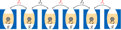
Figure 1: (Color online) Sketch of a CCA with a staggered pattern of hopping rates, where $J_{1}=(1+\eta)J$ and $J_{2}=(1-\eta)J$. The protected mode of each cavity can be coupled to a two-level atom with rate $g$.

Each cavity in turn (see Fig. 1) can be coupled to a two-level quantum emitter (atom).

In this and the following three sections, we shall focus on the free field Hamiltonian, i.e., that of an atom-free CCA. We will consider the full setup, including the atoms, starting from Section VI.

The free field Hamiltonian of the staggered CCA is modelled as (we set $\hbar=1$ throughout)

$$\hat{H}_{\mathrm{hop}}=-J\!\sum_{x=1}^{N-1}[1-(-1)^{x}\eta]\,(\hat{a}_{x+1}^{\dagger}\hat{a}_{x}+\mathrm{H.c.}),$$ (1)

where the bosonic ladder operator $\hat{a}_{x}^{\dagger}$ ($\hat{a}_{x}$) creates (annihilates) a photon at the $x$th cavity. Note that for odd (even) $x$ the quantity between square bracket in Eq. (1) equals $J_{1}=(1+\eta)J$ [$J_{2}=(1-\eta)J$], where $J$ sets the hopping scale and $-1\!\leq\!\eta\!\leq\!1$ is a dimensionless distortion parameter (rates will be always expressed in units of $J$). For $\eta=0$, we retrieve the CCA with uniform inter-cavity couplings usually considered in JCH models Makin et al. (2009). We also point out that, since $N$ is even, for $\eta\rightarrow-1^{+}$ the two outermost cavities (corresponding to $x=1$ and $x=N$, respectively) are weakly coupled to the remaining ones (bulk), a property which will be crucial for our goals. In assuming that the free field Hamiltonian is given by Eq. (1), we have neglected the usual on-site contribution $\sum_{x}\omega_{c}\,\hat{a}_{x}^{\dagger}\hat{a}_{x}$ with $\omega_{c}$ being the frequency of the each cavity protected mode, which is equivalent to set the energy scale such that $\omega_{c}=0$.

Our first task is to diagonalize Hamiltonian (1) in the single-photon Hilbert space, which is spanned by the basis $\{|x\rangle\}$ with $|x\rangle=\hat{a}_{x}^{\dagger}|{\rm vac}\rangle$ and $|{\rm vac}\rangle$ being the field vacuum state. Recalling that $N$ is even, Hamiltonian $\hat{H}_{\rm hop}$ evidently enjoys a mirror symmetry with respect to its middle point, i.e., it is invariant under the transformation $\hat{P}|x\rangle=|N-x+1\rangle$, where $\hat{P}$ is the parity operator. Thereby, $\hat{H}_{\rm hop}$ can be block-diagonalized, each block corresponding to a subspace of a given parity (even or odd). The even (odd) subspace is $N/2$-dimensional and spanned by the basis $\{\left|x\right>_{+}\}$ ($\{\left|x\right>_{-}\}$) with $|x\rangle_{\pm}=(\left|x\right>\!\pm\!\left|N-x+1\right>)/\sqrt{2}$, where $x$ runs from 1 to $N/2$. For now, we add the requirement that the number of cavities is such that $N/2$ must be odd, which is equivalent to demand that $N$ – besides being even – is not an integer multiple of 4 (for our purposes, this is only a mild restriction).

It is straightforward to check that the parity subspaces introduced above yield an effective representation of Hamiltonian (1) given by

$$\hat{H}_{\mathrm{hop}}^{(\pm)}=-J\!\!\!\sum_{x=1}^{N/2-1}\!\!\![1\!-\!(-1)^{x}\eta]\,(\hat{a}_{x+1}^{(\pm){\dagger}}\hat{a}_{x}^{(\pm)}+\mathrm{H.c.})\!\mp\!J_{1}\hat{a}_{N/2}^{(\pm){\dagger}}\hat{a}_{N/2}^{(\pm)}$$ (2)

with $\hat{a}^{(\pm){\dagger}}|{\rm vac}\rangle=|x\rangle_{\pm}$ (if $N/2$ is even, an analogous expression holds but replacing $J_{1}\!\rightarrow\!J_{2}$ on the last term). Note that, unlike in Fig. 1 where the outermost couplings are equal to $J_{1}$, here the leftmost and rightmost couplings are $J_{1}$ and $J_{2}$, respectively. Thus, Hamiltonian $\hat{H}_{\mathrm{hop}}^{(\pm)}$ describes an effective array comprising an odd number of cavities featuring a staggered pattern of hopping rates and a defect at the rightmost cavity $x=N/2$. This defect consists in a local-frequency shift $\mp J_{1}$.

For convenience, let us define $M=N/2$ and $\hat{V}_{\pm}=\mp J_{1}\hat{a}_{M}^{(\rm\pm)\dagger}\hat{a}_{M}^{(\pm)}$, where the latter describes the defect term in Eq. 2. We can now tackle the problem perturbatively by interpreting $\hat{V}_{\pm}$ as a perturbation on a defect-free staggered CCA consisting of an odd number of cavities, a model which can be exactly solved in the single-excitation subspace Ciccarello (2011).

II.1 Diagonalization of $\hat{H}_{\mathrm{hop}}^{(\pm)}$ for $\hat{V}_{\pm}=0$

Based on Ref. Ciccarello (2011), for $\hat{V}_{\pm}=0$ (no defect) the spectrum of $\hat{H}_{\mathrm{hop}}^{(\pm)}$ comprises a pair of bands (separated by a gap $\Delta\omega$) alongside a discrete frequency $\omega_{b}=0$ falling on the middle of the gap. The latter corresponds to a bound eigenstate $|\alpha_{b}\rangle$, which is localized in the vicinity of only one of the array edges (which of the two depends on the sign of $\eta$). This reads

$$|\alpha_{b}\rangle=\mathcal{C}\sum_{x=1}^{\frac{M+1}{2}}{\mathcal{D}}^{x-1}|2x-1\rangle_{\pm}\,$$ (3)

with

$$\mathcal{D}=\frac{J_{1}}{J_{2}}=\frac{1+\eta}{1-\eta}\,,\,\,\,\,\,\,\mathcal{C}=\frac{2}{\eta\!-\!1}\sqrt{\frac{\eta}{\mathcal{D}^{M\!+\!1}\!-\!1}}\,,\,\,$$ (4)

where $\mathcal{D}$ can be interpreted as the distortion ratio. Note that the spatial amplitude of the bound mode, ${}_{\pm}\langle x|\alpha_{b}\rangle$, decays exponentially as $x$ moves away from the weakly-coupled edge. Also, ${}_{\pm}\langle x|\alpha_{b}\rangle=0$ for even $|x\rangle_{\pm}$.

All the remaining eigenvalues, instead, are given by $\omega_{k\mu}=-\mu E_{k}$ with $\mu=\pm$ (band index) and

$$E_{k}=2J\sqrt{\mathrm{cos}^{2}\frac{k}{2}+\eta^{2}\mathrm{sin}^{2}\frac{k}{2}}\,,$$ (5)

where $k=2\pi j/(M+1)$ for $j=1,2,\cdot\!\cdot\!\cdot,(M-1)/2$. These describe a pair of energy bands separated by a band gap $\Delta\omega\leq 4J$, with the identity holding only when $|\eta|=1$ The eigenstates corresponding to $\omega_{k\mu}$ are worked out as Ciccarello (2011)

$$|\alpha_{k\mu}\rangle =\sqrt{\frac{2}{M+1}}\left(\sum_{x=1}^{\frac{M-1}{2}}\mathrm{sin}(kx)|2x\rangle_{\pm}\right.$$

$$\quad+\left.\mu\sum_{x=1}^{\frac{M+1}{2}}\mathrm{sin}(kx+\vartheta_{k})|2x-1\rangle_{\pm}\right),$$ (6)

where the phase $\vartheta_{k}$ is defined by the identity $e^{i\vartheta_{k}}={J(1-\eta)}(e^{-ik}-\mathcal{D})/{E_{k}}$.

II.2 Peturbative diagonalization of $\hat{H}_{\mathrm{hop}}^{(\pm)}$

Let us now tackle the full problem of diagonalizing $\hat{H}_{\mathrm{hop}}^{\pm}$ (taking the defect into account). If $J_{1}\!\ll\!J_{2}$, meaning that the end cavities are weakly coupled to the bulk (see Fig. 1), $\hat{V}_{\pm}$ can be treated as a small perturbation. Applying standard first-order perturbation theory, the bound-mode frequency $\omega_{b}=0$ is then straightforwardly corrected as

$$\omega_{b_{\pm}} \!\simeq\! \omega_{b}\!\mp\!J_{1}\langle\alpha_{b}|\hat{a}_{M}^{(\rm\pm)\dagger}\hat{a}_{M}^{(\pm)}|\alpha_{b}\rangle=\mp\!\dfrac{4J\eta\mathcal{D}^{M}}{(\eta-1)(\mathcal{D}^{M+1}-1)}\,,\,\,\,\,\,\,\,\,$$ (7)

where terms $\sim\!O(J_{1}^{2})$ have been neglected. The perturbation thereby splits $\omega_{b}$ into two discrete frequencies separated by the energy gap

$$\delta\omega=\omega_{b_{-}}-\omega_{b+}=\dfrac{8J\eta}{\eta-1}\,\,\,\frac{\left(\frac{1+\eta}{1-\eta}\right)\!^{N/2}}{\left(\frac{1+\eta}{1-\eta}\right)\!^{N/2+1}-1}\,,\,\,\,\,\,\,\,\,$$ (8)

where we used Eqs. (4) and (7) and replaced $M=N/2$.

The corresponding eigenstates are evaluated as

$$|\alpha_{b_{\pm}}\rangle \simeq|\alpha_{b}\rangle\mp J_{1}\sum_{k,\mu}\frac{\langle\alpha_{k\mu}|\hat{a}_{M}^{\dagger}\hat{a}_{M}|\alpha_{b}\rangle}{\omega_{b}-\omega_{k\mu}}|\alpha_{k\mu}\rangle$$

$$=|\alpha_{b}\rangle\mp 4J\mathcal{C}\left(\dfrac{\eta+1}{M+1}\right)\mathcal{D}^{\frac{M-1}{2}}\sum_{k}\sum_{x=1}^{\frac{M-1}{2}}\dfrac{\mathrm{sin}(kx)}{E_{k}}$$

$$\quad\times\,\mathrm{sin}\left[\left(\dfrac{M+1}{2}\right)k+\vartheta_{k}\right]|2x\rangle_{\pm}.$$ (9)

The unbound states of $\hat{H}_{\mathrm{hop}}^{(\pm)}$ can be easily obtained as well though they yield extensive expressions which we do not report here for the sake of brevity. In Fig. 2, we consider the paradigmatic instance $\eta=-0.25$ and $N=50$, and display the energy spectrum of the full Hamiltonian (1) alongside the spatial profile of the bound states (II.2) on the actual array (i.e., in the basis $\{|x\rangle\}$). We see that the two localized bound states are well-isolated from the unbound modes (the latter corresponding to the pair of bands). They exhibit an energy splitting $\delta\omega$ that, although negligible compared to the band gap $\Delta\omega$, is non-zero. Moreover, each bound state is strongly localized in the vicinity of the array edges (i.e., cavities $x=1$ and $x=N$), a property which from now on we refer to as bi-localization. Those features are key sources for performing QST, as we discuss next.

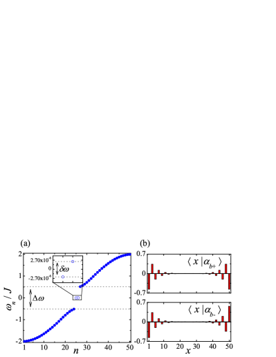
Figure 2: (Color online) (a) Single-excitation spectrum of Hamiltonian (1) (in units of $J$). $\Delta\omega$ is the gap between the pair of bands corresponding to unbound states, while $\delta\omega=\omega_{b-}-\omega_{b+}$ (displayed in the inset) is the energy gap between the localized bound states [cf. Eq. (8)]. (b) Spatial profile of $|\alpha_{b\pm}\rangle$. The plots were obtained by exact numerical diagonalization of Eq. (1) for $\eta=-0.25$ and $N=50$ (comparison with perturbation theory Eqs. (7) and (II.2) is found to be excellent).

III Quantum-state transfer: review

QST protocols are typically formulated in one-dimensional XX-type spin chains, which can be described in terms of ladder spin operators yielding a Hamiltonian of the general form

$$\hat{H}_{\rm ch}=\sum_{x=1}^{N}B_{x}\hat{\sigma}_{x}^{+}\hat{\sigma}_{x}^{-}{+}\sum_{x=1}^{N-1}J_{x}\left(\hat{\sigma}_{x+1}^{+}\hat{\sigma}_{x}^{-}+{\rm H.c.}\right)\,,$$ (10)

where $B_{x}$ is a local effective magnetic field and $\hat{\sigma}_{x}^{+}{=}[\hat{\sigma}_{x}^{-}]^{\dagger}=|1\rangle_{x}\!\langle 0|$ with $\{|0\rangle_{x}$, $|1\rangle_{x}\}$ being a single-spin orthonormal basis. Note that Hamiltonian (10) conserves the total number of excitations, i.e., $[\sum_{x}\hat{\sigma}^{+}_{x}\hat{\sigma}^{-}_{x},\hat{H}_{\rm ch}]=0$. In the single-excitation subspace, the Hamiltonian reduces to a tridiagonal matrix describing a standard hopping model.

III.1 Basics of QST

In the usual QST scheme Bose (2003), the sender prepares an arbitrary qubit state $|\phi\rangle_{1}=c_{0}|0\rangle_{1}+c_{1}|1\rangle_{1}$ at the first site and sets the rest of the chain to $|0\rangle_{2}\cdots|0\rangle_{N}$. The initial state of the whole chain thus reads $|\Psi(0)\rangle=|\phi\rangle_{1}|0\rangle_{2}\cdots|0\rangle_{N}$. The system then evolves according to its Hamiltonian $\hat{H}_{\rm ch}$ so that at time $t$ its state is given by $|\Psi(t)\rangle=\hat{U}(t)|\Psi(0)\rangle$ with $\hat{U}(t)=e^{-i\hat{H}_{\rm ch}t}$. The goal is to exploit such natural dynamics for transferring the initial sender’s state $|\phi\rangle$ to the $N$th spin (receiver) in a given time $\tau$, meaning that $|\Psi(\tau)\rangle=|0\rangle_{1}\cdots|0\rangle_{N-1}|\phi\rangle_{N}$. The received (generally mixed) state is evaluated by tracing out the remaining spins, i.e., $\rho_{N}(\tau)=\mathrm{Tr}_{1,\ldots,N-1}|\Psi(\tau)\rangle\langle\Psi(\tau)|$. One thus aims at making the QST fidelity $F_{\phi}(\tau)=\langle\phi|\rho_{N}(\tau)|\phi\rangle$ as large as possible (the fidelity $F_{\phi}$ measures how close is the receiver’s state to $|\phi\rangle$).

The fidelity introduced above depends on the specific input $|\phi\rangle$. In order to end up with a state-independent figure of merit for QST, one needs to average $F_{\phi}$ over all possible input states on the Bloch sphere ($|c_{0}|^{2}+|c_{1}|^{2}=1$). For Hamiltonians of the form (10), which conserves the total number of excitations, and given that $|\Psi(0)\rangle$ is restricted to evolve in the zero- and one-excitation subspaces, the former being unaffected by $U(t)$, the average fidelity is simply given by Bose (2003)

$$\mathcal{F}(t)=\frac{1}{2}+\frac{|f(t)|}{3}+\frac{|f(t)|^{2}}{6}~{}\,,$$ (11)

where

$$f(t)=\langle N|e^{-i\hat{H}_{\rm ch}t}|1\rangle$$ (12)

is the excitation transition amplitude from the first to the last spin. (we used the compact notation $|x\rangle\equiv\hat{\sigma}_{x}^{+}|0\rangle_{1}\cdots|0\rangle_{N}$). Note that $|f(\tau)|=1$ entails $\mathcal{F}(\tau)=1$ (perfect QST). Also, the average fidelity is a monotonic function of the transition amplitude and hence the QST performance can be evaluated by just tracking down the excitation transport across the array.

When the state to be transferred is encoded in more than two levels (a qutrit for instance) and/or the chain is not properly initialized (thus containing unwanted excitations), the average fidelity is not expressed by Eq. (11), even though it still depends on the involved transition amplitudes Latmiral et al. (2015); Lorenzo et al. (2015).

III.2 Rabi-like QST

In the single-excitation sector, the spectral decomposition of Hamiltonian (10) reads $\hat{H}_{\mathrm{ch}}=\sum_{j=1}^{N}\omega_{j}|\upsilon_{j}\rangle\!\langle\upsilon_{j}|$, where $\omega_{j}$ is the $j$th energy eigenvalue with corresponding eigenstate $|\upsilon_{j}\rangle=\sum_{j=1}^{N}\upsilon_{jx}|x\rangle$. In this representation, the transition amplitude discussed above is given by

$$f(t)=\sum_{j=1}^{N}e^{-i\omega_{j}t}\upsilon^{*}_{jN}\upsilon_{j1}=\sum_{j=1}^{N}e^{-i\omega_{j}t}\langle\upsilon_{j}|\hat{\sigma}_{1}^{+}\hat{\sigma}^{-}_{N}|\upsilon_{j}\rangle.\,\!\!\!\!\!$$ (13)

The last identity shows that each eigenstate contributes to Eq. (13) through the quantity $\langle\upsilon_{j}|\hat{\sigma}_{1}^{+}\hat{\sigma}^{-}_{N}|\upsilon_{j}\rangle$, evolving in time at rate $\omega_{j}$. In the remainder of this paper, we will refer to it as the end-to-end amplitude.

Various high-quality QST schemes Plastina and Apollaro (2007); Linneweber et al. (2012); Lorenzo et al. (2013); Wójcik et al. (2005); Huo et al. (2008) rely on the situation where the edge states $|1\rangle$ and $|N\rangle$ have a strong overlap with only two stationary states, say those indexed by $j=1,2$ (bi-localization). In this case, Eq. (13) can be approximated as

$$f(t)\simeq e^{-i\frac{\delta\omega\,t}{2}}\langle\upsilon_{1}|\hat{\sigma}_{1}^{+}\hat{\sigma}^{-}_{N}|\upsilon_{1}\rangle+e^{i\frac{\delta\omega\,t}{2}}\langle\upsilon_{2}|\hat{\sigma}_{1}^{+}\hat{\sigma}^{-}_{N}|\upsilon_{2}\rangle$$ (14)

with $\delta\omega=\omega_{1}-\omega_{2}$ (we assumed $\omega_{1}>\omega_{2})$. This entails a Rabi-like dynamics that occurs with a characteristic Rabi frequency given by $\delta\omega$. Accordingly, $\tau\sim\delta\omega^{-1}$ showing that the order of magnitude of the transmission time is set by the energy gap between the two bi-localized eigenstates.

The above bi-localization effect is usually achieved by introducing perturbation terms in the Hamiltonian that decouple the outermost spins from the bulk. This can be realized through: (i) application of strong local magnetic fields on the edge spins Plastina and Apollaro (2007); Linneweber et al. (2012), or (ii) on their nearest-neighbours Lorenzo et al. (2013), and (iii) engineering of weak couplings between the edge spins and bulk Wójcik et al. (2005); Huo et al. (2008). While all these models share that a pair of Hamiltonian eigenstates exhibit strong bi-localizaton on the edge sites, the typical energy gap between such two states – and accordingly the transmission time – depend on the considered model. Calling $\xi$ the model-dependent perturbation parameter (such as the local magnetic field strength), in (i) the time scales with $N$ as $\tau\sim\xi^{N}$, resulting in a QST time that exponentially increases with the array length, whereas in (ii) and (iii) the time scales as $O(\xi^{2})$ and $O(\xi^{-2})$, respectively. All those typical transfer times are in general relatively long and may easily exceed the system’s coherence time scale. Therefore, it is of great importance to design protocols demanding shorter transfer times.

IV QST in atom-free staggered CCAs

Comparing Eqs. (1) and (10), it should be evident that within the single-excitation subspace, one can regard the spin chain as an atom-free CCA. Indeed, in such a case the mapping is straightforward and reads $\hat{\sigma}_{x}^{+}\rightarrow\hat{a}_{x}^{\dagger}$, $\hat{\sigma}_{x}^{-}\rightarrow\hat{a}_{x}$. Likewise, the QST protocol previously discussed in Section III.1 now takes place in the zero- and one-photon sectors $\{|{\rm vac}\rangle,\,|x\rangle\}$. Until Section V we will thus address QST along a staggered CCA with no atoms. This will introduce one of our main results of Section V, where we show that the staggered CCA QST time can be significantly reduced by adding modularization on top of the staggered scheme. On the one hand, this analysis provides the necessary basis for QST on CCAs coupled to atoms, which we will investigate starting from Section VI. On the other hand, it has its own relevance since our findings are independent of the CCA-based implementation, hence they apply to any spin chain with an analogous pattern of couplings.

In the light of Sections II and III, the atom-free staggered array is suitable for implementing QST based on bi-localization (see Section III.2) in the regime $J_{1}\ll J_{2}$. To see this, consider first the limiting case $J_{1}=0$, i.e., $\eta=-1$. In this limit (dimerization), the array reduces to a pair of isolated cavities at the outermost sites and a bulk of uncoupled dimers [see the small sketch on top of Fig. 3(a)]. The pair of bound states [cf. Eq. (II.2)] then reduce to the doublet $|\alpha_{b\pm}\rangle=(|1\rangle\pm|N\rangle)/\sqrt{2}$ with $\omega_{b_{\pm}}=0$, these being evidently the only stationary states with non-zero amplitude at the array ends. This would turn Eq. (14) into an exact identity with $\{|\alpha_{b\pm}\rangle\}$ embodying the pair $\{|\upsilon_{1}\rangle,|\upsilon_{2}\rangle\}$. Yet, due to $\omega_{b_{\pm}}=0$, the transmission time $\tau$ would be infinite since $\delta\omega=0$. To make this finite, we thus need to work in the regime $J_{1}\!\ll\!J_{2}$, which justifies our perturbative approach in Section II.2.

Next, with the help of Eqs. (3) and (II.2), we note that the end-to-end amplitudes entering Eq. (14) fulfill

$$\langle\alpha_{b\pm}|\hat{a}_{1}^{\dagger}\hat{a}_{N}|\alpha_{b\pm}\rangle=\pm\tfrac{\mathcal{C}^{2}}{2}+O(J_{1}^{2})\,.$$ (15)

Thereby, the transition amplitude’s modulus reads

$$|f(t)|=2\left|\langle\hat{a}_{1}^{\dagger}\hat{a}_{N}\rangle\,\mathrm{sin}\left(\dfrac{\delta\omega}{2}t\right)\right|,$$ (16)

where $\langle\hat{a}_{1}^{\dagger}\hat{a}_{N}\rangle$ is a short notation for the end-to-end amplitude. At times $t=2n\pi/\delta\omega$ with $n$ being an odd integer, Eq. (16) reaches the value $2|\langle\hat{a}_{1}^{\dagger}\hat{a}_{N}\rangle|$. Hence, ideally, if the absolute value of the end-to-end amplitude equals 1/2, perfect QST is attained with transmission time $\tau=2\pi/\delta\omega$.

In Fig. 3(a), based on exact numerical diagonalization of Eq. (1), we explore how the end-to-end amplitude is affected by the array size $N$ and $J_{1}/J_{2}$.

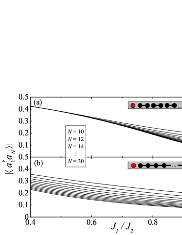
Figure 3: (Color online) End-to-end amplitude $|\langle\alpha_{b\pm}|\hat{a}_{1}^{\dagger}\hat{a}_{N}|\alpha_{b\pm}\rangle|$ vs. $J_{1}/J_{2}$ for several values of $N$ (in increasing order from top to bottom) in the case of a staggered array (a) described by Hamiltonian (1) and a uniform bulk (b) described by Hamiltonian (17). Note that $J_{1}/J_{2}$ decreases from right to left. Each plot is obtained from an exact numerical diagonalization of the Hamiltonian.

For a set ratio $J_{1}/J_{2}$, the amplitude decreases with $N$, eventually saturating to an asymptotic value. For $J_{1}/J_{2}=1$ (uniform hopping rates) the asymptotic value is well below 1/2 but tends to it as $J_{1}/J_{2}$ approaches zero. At the same time, remarkably, the rapidity at which $|\langle\hat{a}_{1}^{\dagger}\hat{a}_{N}\rangle|$ saturates to such asymptotic value as a function of $N$ grows up in a way that, for $J_{1}/J_{2}$ small enough, the amplitude becomes in fact $N$-independent. This agrees with Eq. (15) [see also Eq. (4)].

In other words, for a very distorted array, the bi-localization effect required for high-fidelity QST is about insensitive to the system size. This property is related to what is known as true long-distance entanglement exhibited by the ground state of staggered spin chains Campos Venuti et al. (2007b), as opposed to quasi-long-distance entanglement featuring quantum correlations that decrease with $N$. The latter occurs, for instance, in spin chains comprising a uniform bulk Wójcik et al. (2005); Campos Venuti et al. (2007b). The fundamentally different nature of those two situations reflects in the scaling properties of QST fidelity as well. To show this, consider a CCA where – unlike the staggered array – the bulk cavities are coupled uniformly with rate $J_{2}$ [see sketch on top of Fig. 3(b)]. The Hamiltonian of such an array thus reads

$$\hat{H}_{\mathrm{hop}}^{\prime}=-J_{1}(\hat{a}_{2}^{\dagger}\hat{a}_{1}+\hat{a}_{N}^{\dagger}\hat{a}_{N-1})-J_{2}\!\sum_{x=2}^{N-2}\hat{a}_{x+1}^{\dagger}\hat{a}_{x}+\mathrm{H.c.}$$ (17)

Since the outermost sites are weakly coupled to the bulk, a pair of bi-localized eigenstates is formed in this case too Wójcik et al. (2005). In Fig. 3(b), we plot the corresponding end-to-end amplitude as a function of $J_{1}/J_{2}$ and $N$. The differences with respect to the staggered-CCA case are quite striking. While for $J_{1}/J_{2}=1$ (fully uniform array) both models coincide, the end-to-end amplitude in the uniform-bulk case decreases with $N$ at variance with the stable behaviour found in the staggered model, taking moreover lower values compared to the latter. This shows some of the attractive features of staggered arrays in terms of QST fidelity.

V Modularized array

The advantages highlighted in the previous section, however, come with a price in terms of the transmission time $\tau$ required for carrying out QST. Recalling that $\tau\sim\delta\omega^{-1}$, Eq. (8) indeed shows that, in the regime $J_{1}\!\ll\!J_{2}$ (i.e., $\eta\!\simeq\!-1$), the bound-state gap $\delta\omega$ exponentially decays with the size $N$. As a consequence, $\tau$ exponentially grows up with $N$. One thus wonders whether, for a given size, the staggered array can be modified so as to increase the gap while maintaining the bi-localization strength of $|\alpha_{b\pm}\rangle$ (necessary to attain high fidelity). In this section, we show that this can be achieved by modularizing the staggered CCA.

The setup we put forward is inspired by the concept of modular entanglement introduced in Ref. Gualdi et al. (2011). Let us consider then a set of $m$ identical staggered arrays, having $N$ sites each, so that the total number of sites is $L=mN$. Nearest-neighbour cavities of adjacent modules are coupled with hopping rate $J_{\rm mod}$, hence the total Hamiltonian reads

$$\hat{H}_{\mathrm{mod}}=\sum_{j=1}^{m}\hat{H}_{\mathrm{hop}}^{(j)}-J_{\mathrm{mod}}\!\sum_{j=1}^{m-1}(\hat{a}_{jN+1}^{\dagger}\hat{a}_{jN}+\mathrm{H.c.})\,,$$ (18)

where the free module Hamiltonian $\hat{H}_{\mathrm{hop}}^{(j)}$ is the same as Eq. (1) [the sum being now over $x=(j\!-\!1)N+1,jN-1$].

For $J_{\rm mod}=J_{2}$, the whole setup reduces to a standard staggered array comprising $L$ cavities. In contrast, in the limit $J_{\rm mod}=0$ (no inter-modular couplings), the energy spectrum and associated eigenstates of $\hat{H}_{\rm mod}$ are the same as those of a single $N$-long module analyzed in Section II, but becoming $m$-fold degenerate. For intermediate values $0<J_{\rm mod}<J_{2}$, such degeneracy is removed resulting in a manifold of 2$m$ non-degenerate bound states. Among these, let us call $\delta\omega_{m,N}$ the energy gap between the pair of most internal ones and $|\langle\hat{a}_{1}^{\dagger}\hat{a}_{L}\rangle|$ the absolute value of their end-to-end amplitude. Then, for $J_{\rm mod}=J_{2}$, $\delta\omega_{m,N}$ and $|\langle\hat{a}_{1}^{\dagger}\hat{a}_{L}\rangle|$ are respectively the same as $\delta\omega$ and the corresponding end-to-end amplitude of a staggered array of size $L$ [see Eq. (8) and Fig. 3(a)]. In the opposite limit $J_{\rm mod}=0$, $\delta\omega_{m,N}$ is larger, since now it coincides with the bound-state gap of a staggered array of size $N\!<\!L$, while $|\langle\hat{a}_{1}^{\dagger}\hat{a}_{L}\rangle|=0$ because the modules are now uncoupled.

To investigate the dependence of $\delta\omega_{m,N}$ and $|\langle\hat{a}_{1}^{\dagger}\hat{a}_{L}\rangle|$ on $J_{\rm mod}$, in Fig. 4 we consider the cases of a two- and three-module array ($\delta\omega_{m,N}$ is plotted in units of $\delta\omega_{1,L}$, namely its value at $J_{\rm mod}=J_{2}$). As $J_{\rm mod}$ grows from zero, both the gap and the end-to-end amplitude monotonically tend to their respective values for $J_{\rm mod}=J_{2}$ (i.e., the case discussed above). Remarkably, the end-to-end amplitude in particular exhibits quite a fast saturation [see Figs. 4(a) and (b)]. Instead, $\delta\omega_{m,N}$ undergoes a more regular growth. This means that, starting from $J_{\rm mod}=J_{2}$ ($L$-size staggered array) one can decrease $J_{\rm mod}$ by a significant amount – thus modularizing the CCA – and keep the end-to-end amplitude about unchanged but amplifying the energy gap substantially. For instance [see Figs. 4(a) and (c)], in the two-module ($m=2$) case for $N=14$ when $J_{\rm mod}\simeq 0.01J$ the end-to-end amplitude is unchanged for all practical purposes while the energy gap is over a hundred times larger, resulting in the same QST fidelity but with a transfer time about two orders of magnitude lower. This can be further improved by increasing the number of modules, for fixed overall array length $L$ since this results in modules of shorter length.

Figure 4: (Color online) Full-array end-to-end amplitude $|\langle\hat{a}_{1}^{\dagger}\hat{a}_{L}\rangle|$ [(a) and (b)] and energy-gap gain $\delta\omega_{m,N}/\delta\omega_{1,L}$ [(c) and (d)] against $J_{\mathrm{mod}}/J$ for different values of $N$ in the case of a modularized staggered CCA. Left-column plots [(a) and (c)] refer to a two-module array ($m=2$), while right-column ones [(b) and (d)] correspond to a three-module array ($m=3$). For each setup, we have set the intra-module distortion to $\eta=-0.5$ (about $J_{1}/J_{2}=0.33$).

We also note from Fig. 4 that the saturation of $|\langle\hat{a}_{1}^{\dagger}\hat{a}_{L}\rangle|$ occurs for lower values of $J_{\rm mod}$ as $N$ grows. Hence, lower values of $J_{\rm mod}$ are required for establishing bi-localization. This can be attributed to the fact that the gap $\delta\omega$ of each (isolated) staggered module, coinciding with $\delta\omega_{m,N}$ for $J_{\rm mod}=0$, decreases with $N$. From a perturbative perspective, the effect of switching on an inter-modular coupling will be significant when $J_{\rm mod}$ becomes comparable with $\delta\omega$ which, however, decreases with $N$.

To summarize, for a staggered array of a given length, partitioning it into several module can result in shorter QST times without significantly affecting the corresponding fidelity. In Fig. 5, we provide further explicit evidence of this phenomenon by considering a CCA of length $L=24$ in the case of four different modularizations defined by $m=2,3,4,$ and 6. Note, for instance, that a six-block modularization leaves the fidelity above $\simeq 95\%$ while the QST time is shortened by three orders of magnitude. A significant QST speed-up is nevertheless attainable even for lower $m$. Note that while the QST time increases polynomially with $J_{\mathrm{mod}}$, the fidelity shows a non-monotonic behavior due to residual contributions from other eigenstates to the transition amplitude [see Eq. (13)].

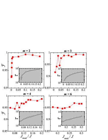
Figure 5: (Color online) Maximum achievable average QST fidelity $\mathcal{F}$ [cf. Eq. 11)] after one Rabi-like oscillation period, that is $\tau=2\pi/\delta\omega_{m,N}$, against $J_{\rm mod}/J$. We have set $L=24$, $J_{1}=0.3J$ and $J_{2}=J$ and considered different modularization schemes (each specified by the value of $m$). In each panel, the inset shows the transfer time $\tau$ (in units of $J^{-1}$) vs. $J_{\rm mod}/J$ in a log-lin scale. For the unmodularized array ($m=1$), the maximum fidelity and transfer time are, respectively, $\mathcal{F}\simeq 0.98$ and $\tau\simeq 3\cdot 10^{6}J^{-1}$.

The possibility to reduce QST times over relatively short distances – say of the order of up to 30 sites as in Fig. 5 – is relevant itself, e.g., to carry out short-haul communications tasks between quantum processors in a quantum computing architecture. Concerning longer CCAs, a thorough analysis of the scalability of a modularized array is beyond the scopes of the present work and will thus be presented elsewhere Almeida et al. . However, in order to test the potential of modularized chains to perform QST over longer distances, in Fig. 6 we additionally consider the paradigmatic case of a CCA having $L\!=\!102$ sites. Note that high-quality QST is still achievable within times that, although inevitably longer, are far shorter compared to the unmodularized staggered CCA.

Figure 6: (Color online) Maximum achievable average QST fidelity $\mathcal{F}$ [cf. Eq. 11)] after one Rabi-like oscillation period, that is $\tau=2\pi/\delta\omega_{m,N}$, against $J_{\rm mod}/J$. We have set $L=102$ and $\eta=-0.8$ (about $J_{1}/J_{2}=0.11$) using the modularization scheme $m=17$, the length of each module thus being $N=6$. The inset shows the transfer time $\tau$ (in units of $J^{-1}$) vs. $J_{\rm mod}/J$ in a log-lin scale. For the corresponding unmodularized CCA, the transfer time is infinite for all pratical purposes.

As mentioned previously, all the above clearly applies not only to atom-free CCAs, but spin chains in general (regardless of their implementation). In the following, we will address CCAs coupled to atoms with the goal of putting forward QST schemes in which both atomic and photonic degrees of freedom are involved.

VI CCA with atoms

We now consider a CCA, where each cavity is additionally coupled to a two-level atom of frequency $\omega_{a}$, according to the Jaynes-Cummings (JC) interaction Hamiltonian Jaynes and Cummings (1963)

$$\hat{H}_{x}^{(\mathrm{JC})}=\omega_{c}\hat{a}_{x}^{\dagger}\hat{a}_{x}+\omega_{a}\hat{\sigma}_{x}^{+}\hat{\sigma}_{x}^{-}+g\,(\hat{\sigma}_{x}^{+}\hat{a}_{x}+\hat{\sigma}_{x}^{-}\hat{a}_{x}^{\dagger}),$$ (19)

where now $\hat{\sigma}_{x}^{+}\equiv|\mathrm{e}\rangle_{x}\!\langle\mathrm{g}|$ with $|\mathrm{g}\rangle$ ($|\mathrm{e}\rangle$) denoting the atomic ground (excited) state, and $g$ is the atom-field coupling strength. In the following, we again set $\omega_{c}=0$ for simplicity. For a staggered pattern of hopping rates (see Fig. 1), the total Hamiltonian reads

$$\hat{H}=\hat{H}_{\mathrm{hop}}+\sum_{x=1}^{N}\hat{H}_{x}^{\mathrm{(JC)}},$$ (20)

where the hopping Hamiltonian is the same as in Eq. (1). Hereafter, we adopt the short notation $|1_{x}\rangle\equiv\hat{a}_{x}^{\dagger}|\mathrm{vac}\rangle|\mathrm{g}\rangle_{1}\cdots|\mathrm{g}\rangle_{N}$ and $|e_{x}\rangle\equiv\hat{\sigma}_{x}^{+}|\mathrm{vac}\rangle|\mathrm{g}\rangle_{1}\cdots|\mathrm{g}\rangle_{N}$, where the former is the state where a single photon lies at the $x$th cavity with all the atoms unexcited, while in the latter state only the $x$th atom is excited (with the field and all of the remaining atoms unexcited). The single-excitation sector of the joint Hilbert space is 2$N$-dimensional and spanned by the basis $\{|1_{x}\rangle,|e_{x}\rangle\}$.

Moreover, let us denote $\{|\alpha_{n}\rangle\}$ as the set of $N$ eigenstates of the free field Hamiltonian $\hat{H}_{\rm hop}$, i.e., $\hat{H}_{\rm hop}|\alpha_{n}\rangle=\omega_{n}|\alpha_{n}\rangle$, each having the form $|\alpha_{n}\rangle=\sum_{x}\alpha_{nx}\left|1_{x}\right>$. These states solely comprise photonic excitations (index $n$ is intended to run over both bound and unbound states). Correspondingly, one can define a set of $N$ states $\{|\beta_{n}\rangle\}$ such that $|\beta_{n}\rangle=\sum_{x}\alpha_{nx}\left|e_{x}\right>$, hence featuring only atomic excitations (excitons). By construction, each $|\beta_{n}\rangle$ has the same spatial profile as $|\alpha_{n}\rangle$ and can thus be regarded as its excitonic analogue. States $\{|\alpha_{n}\rangle\}$ ($\{|\beta_{n}\rangle\}$) can be regarded as arising from the normal-mode field (atomic) operators $\{\hat{\alpha}_{n}\}$ ($\{{\hat{\beta}_{n}}\}$) defined accordingly as $\hat{\alpha}_{n}=\sum_{x}\alpha_{nx}\hat{a}_{x}$ ($\hat{\beta}_{n}=\sum_{x}\alpha_{nx}\hat{\sigma}_{x}^{-}$).

Note that in Eq. (20) both $g$ and $\omega_{a}$ are uniform throughout the array. Using this, $\hat{H}$ can be rearranged as (see Refs. Ogden et al. (2008); Makin et al. (2009); Ciccarello (2011))

$$\hat{H}=\!\sum_{n}\left[\omega_{n}\hat{\alpha}_{n}^{\dagger}\hat{\alpha}_{n}+\omega_{a}\hat{\beta}_{n}^{\dagger}\hat{\beta}_{n}+g(\hat{\beta}_{n}^{\dagger}\hat{\alpha}_{n}+{\rm H.c.})\right]\,.$$ (21)

Therefore, within the single-excitation sector, the system behaves as a set of $N$ decoupled effective JC models, each corresponding to a photonic mode of frequency $\omega_{n}$ coupled to its excitonic counterpart of frequency $\omega_{a}$ with coupling strength $g$. This allows for a straightforward diagonalization of $\hat{H}$ once the eigenstates of the free field Hamiltonian $\hat{H}_{\rm hop}$, $\{|\alpha_{n}\rangle\}$, are known. Using the standard JC-model theory, indeed, the eigenstates are worked out as

$$|\psi_{n}^{(\pm)}\rangle=A_{n}^{(\pm)}\left|\alpha_{n}\right>+B_{n}^{(\pm)}\left|\beta_{n}\right>,$$ (22)

where

$$A_{n}^{(\pm)}=\dfrac{2g}{\sqrt{(\Delta_{n}\!\pm\!\Omega_{n})^{2}+4g^{2}}},\,\,\,B_{n}^{(\pm)}=\dfrac{\Delta_{n}\!\pm\!\Omega_{n}}{\sqrt{(\Delta_{n}\!\pm\!\Omega_{n})^{2}+4g^{2}}},$$ (23)

with $\Delta_{n}=\omega_{a}-\omega_{n}$ and $\Omega_{n}=\sqrt{\Delta_{n}^{2}+4g^{2}}$ being the detuning and vacuum Rabi frequency, respectively, of the $n$th effective JC model. The corresponding energy levels read

$$\varepsilon_{n}^{(\pm)}=\tfrac{1}{2}\,(\omega_{a}+\omega_{n}\pm\Omega_{n}).$$ (24)

VI.1 Single-mode resonance

Out of all the $N$ effective JC dynamics [cf. Eq. (21)] one can selectively excite only one of them upon a judicious tuning of the atomic frequency $\omega_{a}$. Now we particularly show how to trigger only the JC dynamics corresponding to the bound eigenstate $|\alpha_{b+}\rangle$ [cf. Eq. (II.2)]. In the interaction picture, Hamiltonian (21) is turned into (we now highlight explicitly the contributions of the bound and unbound states)

$$\hat{H}_{\rm I}(t)=g\!\left[\sum_{j=\pm}\!\hat{\beta}_{bj}^{\dagger}\hat{\alpha}_{bj}e^{i\Delta_{bj}t}\!+\!\sum_{k\mu}\!\hat{\beta}_{k\mu}^{\dagger}\hat{\alpha}_{k\mu}e^{i\Delta_{k\mu}t}\!+{\rm H.c.}\right]\,\,\,\,\,\,\,\,\,\,$$ (25)

with $\Delta_{b\pm}=\omega_{a}-\omega_{b\pm}$ and $\Delta_{k\mu}=\omega_{a}-\omega_{k\mu}$. By tuning $\omega_{a}$ on resonance with $\omega_{b+}$, namely setting $\omega_{a}\!=\!\omega_{b+}$ the first term becomes time-independent. If, additionally, $g\!\ll\{\Delta_{k\mu},\Delta_{b-}\}$ all the remaining terms in Eq. (25) are rapidly rotating so that they effectively do not affect the dynamics and, hence, can be neglected. Returning to the Schrödinger picture, we thus end up with an effective Hamiltonian of the form

$$\hat{H}_{\rm eff}=\!\sum_{n}\left(\omega_{n}\hat{\alpha}_{n}^{\dagger}\hat{\alpha}_{n}+\omega_{a}\hat{\beta}_{n}^{\dagger}\hat{\beta}_{n}\right)+g(\hat{\beta}_{b+}^{\dagger}\hat{\alpha}_{b+}+{\rm H.c.})\,.$$ (26)

An analogous conclusion holds if we set the atomic frequency on resonance with $\omega_{b-}$. The dynamics thus consists of a resonant JC-like dynamics involving $|\alpha_{b+}\rangle$ and its excitonic analogue, while all the remaining photonic and atomic modes evolve freely. Accordingly, only the pair of dressed states $|\psi_{b+}^{(\pm)}\rangle$ are thus formed [cf. Eq. (22)]. Note that, due to the resonance condition $\Delta_{b+}=0$, we get $|A_{b+}^{(\pm)}|=|B_{b+}^{(\pm)}|$ [cf. Eq. (23)]. Hence, $|\psi_{b+}^{(\pm)}\rangle$ are fully dressed states featuring maximal atom-photon entanglement.

VI.2 Strong-coupling regime

Clearly, an implicit requirement for the above regime to hold is that $g\!\ll\!\delta\omega$ (since $|\alpha_{b-}\rangle$ is the nearest state in energy). If not, additional coupling terms between field modes and the respective excitonic analogues would appear in Eq. (26). Consider, in particular, the strong-coupling regime Makin et al. (2009); Almeida and Souza (2013) such that $g$ is far larger than the entire range of the field frequencies ($\omega_{a}=0$ for simplicity). Then, none of the coupling terms in Eq. (21) can be neglected in a way that each corresponding JC dynamics is activated. Also, due to the negligible detunings, all the pairs of states in Eq. (22) are formed, each reading $|\psi_{n}^{(\pm)}\rangle\!\simeq\!(\left|\alpha_{n}\right>\pm\left|\beta_{n}\right>)/\sqrt{2}$, thus embodying fully dressed states. Accordingly, the energy spectrum [cf. Eq. (24)] reduces to $\varepsilon_{n}^{(\pm)}\!\simeq{\omega_{n}}/{2}\pm g$ (since $\Omega_{n}\!\simeq\!2g$). Thereby, in this regime two independent polaritonic bands are formed, each corresponding to even (odd) dressed states $|\psi_{n}^{(+)}\rangle$ $(|\psi_{n}^{(-)}\rangle)$. In either of these, the dynamics thus reduces to a single polariton subjected to an effective Hamiltonian that is analogous to the free field hopping Hamiltonian (1) [or (18) in the case of modularization] but with all the hopping rates rescaled by a 1/2 factor. If the CCA is prepared in a state such as $(|e_{1}\rangle\pm|1_{1}\rangle)/\sqrt{2}$, then only the corresponding band will be excited and the dynamics will be the same as that analyzed in previous sections (with each single-photon state $|x\rangle$ now replaced by the single-cavity polariton state $(|e_{x}\rangle\!\pm\!|1_{x}\rangle)/\sqrt{2}$).

VII Transfer of atomic and polaritonic states

Depending on the single-mode resonance or strong-coupling regimes discussed in Sections VI.1 and VI.2, respectively, we now show that one can carry out transfer of an atomic or polaritonic state.

VII.1 Atomic QST through single-mode resonance

Setting $\omega_{a}=\omega_{b+}$ and $g\!\ll\!\delta\omega$, the latter being the gap between the bi-localized states $|\alpha_{b\pm}\rangle$, the JCH Hamiltonian takes the effective form of Eq. (26). If the parameters entering Eq. (1) [or Eq. (18) for modularized CCAs] are such that strong bi-localization occurs (see Sections II, IV, and V), then both the excitonic states $|e_{1}\rangle$ and $|e_{N}\rangle$ can be decomposed to a good approximation only in terms of $|\beta_{b\pm}\rangle$. This gives $|e_{1}\rangle\!\simeq\!\sum_{j=\pm}\langle\beta_{bj}|e_{1}\rangle|\beta_{bj}\rangle$ and, using the parity properties of $|\beta_{b\pm}\rangle$, $|e_{N}\rangle\!\simeq\!-\langle\beta_{b-}|e_{1}\rangle|\beta_{b-}\rangle+\langle\beta_{b+}|e_{1}\rangle|\beta_{b+}\rangle$. Expressing next $|\beta_{b+}\rangle$ in terms of dressed states [see Eq. (22)], we get $|\beta_{b+}\rangle=\tfrac{1}{\sqrt{2}}\left(|\psi_{b+}^{(+)}\rangle-|\psi_{b+}^{(-)}\rangle\right)$, where $|\psi_{b+}^{(\pm)}\rangle$ has energy $\omega_{0}\pm g$. Replacing it into the above decomposition for $|e_{1}\rangle$ and letting this evolve in time through to the usual time-evolution operator $\hat{U}(t)$, we get

$$\hat{U}(t)|e_{1}\rangle \!\simeq\! \langle\beta_{b-}|e_{1}\rangle|\beta_{b-}\rangle$$ (27)

$$+\tfrac{\langle\beta_{b+}|e_{1}\rangle}{\sqrt{2}}\left(e^{-igt}|\psi_{b+}^{(+)}\rangle-e^{igt}|\psi_{b+}^{(-)}\rangle\right)$$

up to an irrelevant global phase factor. Expressing now again the dressed states in terms of $|\alpha_{b+}\rangle$ and $|\beta_{b+}\rangle$,

$$\hat{U}(t)|e_{1}\rangle \!\simeq\! \langle\beta_{b-}|e_{1}\rangle|\beta_{b-}\rangle$$ (28)

$$+\langle\beta_{b+}|e_{1}\rangle\left[\cos(gt)|\beta_{b+}\rangle\!-\!i\sin(gt)|\alpha_{b+}\rangle\right].$$

For $gt=\pi$ (up to an irrelevant global phase factor), we thus get (see above) $\hat{U}(t)|e_{1}\rangle\!\simeq\!|e_{N}\rangle$. Noting that, in the light of Section III, the state in which the CCA has zero excitations (both photonic and atomic) does not evolve, the two-level atom constitutes a natural choice for encoding the logical qubit. Therefore, a QST protocol can be carried out between the outermost atoms in a transfer time $\tau=\pi/g$.

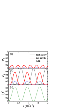
Figure 7: (Color online) Time evolution of the photonic (a) and atomic (b) excitation and of the transition amplitude (c) across a 10-cavity staggered CCA for an initial state $|\Psi(0)\rangle=|e_{1}\rangle$. In (a) [(b)], we display the probability to find the photonic (atomic) excitation at the first cavity (thin black), the last one (thick red), and in the bulk sites $2\!\leq\!x\!\leq\!N-1$ (dashed blue). The plots are obtained from an exact numerical diagonalization of Eq. (20) for $\eta=-0.5$ and $g=10^{-6}J$.

Likewise, one can accordingly define a transition amplitude (cf. Section III) as $f(t)=\langle e_{N}|\hat{U}(t)|e_{1}\rangle$ and evaluate the QST efficiency using Eq. (11) for the average fidelity.

In Fig. 7, we study in a paradigmatic instance (such that $|\Psi(0)\rangle=|e_{1}\rangle$) the time evolution of the photonic and atomic excitations alongside the transition amplitude just introduced. We denote $p_{{\rm f},x}(t)=|\langle 1_{x}|\Psi(t)\rangle|^{2}$ and $p_{{\rm a},x}(t)=|\langle e_{x}|\Psi(t)\rangle|^{2}$ as the probability to find one photon and one exciton at cavity $x$, respectively. As shown in Fig. 7, the transfer takes place through the involvement of the entire CCA, including the bulk (especially in the form of excitons). Note that, while the considered array is only moderately distorted (we take $\eta=-0.5$), $|f|$ attains a maximum $\simeq 0.9$.

VII.2 Polariton transmission in the strong-coupling regime

Note that in the scheme discussed previously, the transfer time $\tau$ is set in fact by the atom-field coupling strength $g$, which is required to be much smaller than the energy gap between bi-localized modes $\delta\omega$. As the latter decreases with the array distortion (see Section II), such a scheme can be demanding for highly-distorted CCAs. In this scenario, the properties of an atom-free CCA as seen in Sections II, IV, and V can be exploited to transfer polaritonic states across the array.

In the strong-coupling regime (see Section VI.2), the dynamics reduces to that of a pair of fully-dressed polaritonic bands. In either of these, a single-cavity polariton of given parity hops through the array just like a photon propagates through an atom-free CCA (see Sections II, IV and V) apart from a 1/2 factor rescaling of hopping rates (hence half of the propagation speed). Given that the polaritonic bands are uncoupled, the preparation of a polariton of a given parity in a given cavity, say $\tfrac{1}{\sqrt{2}}(|e_{1}\rangle+|1_{1}\rangle)$, will trigger a dynamics where solely polaritons of the same parity are involved. Hence, at least in principle, one can encode a qubit in each cavity in terms of atom-photon logical states $|\mathrm{vac}\rangle|\mathrm{g}\rangle_{1}\cdots|\mathrm{g}\rangle_{N}$ and $\tfrac{1}{\sqrt{2}}(|e_{x}\rangle+|1_{x}\rangle)$. Accordingly, in such a framework and in virtue of Section III, this leads to a transition amplitude defined as $f(t)=\tfrac{1}{2}(\langle e_{N}|+\langle 1_{N}|)\hat{U}(t)(|e_{1}\rangle+|1_{1}\rangle)$. Regardless of the feasibility of such a qubit implementation, $f(t)$ can be used as a figure of merit for measuring how reliably a polaritonic state can be transmitted across the CCA in line with other studies Nohama and Roversi (2007); Bose et al. (2007); Ogden et al. (2008); Makin et al. (2009).

Interestingly, in order for the polariton transfer to be effective, the requirement that $g$ must be strong enough in order to enable the entire set of dressed states to form is not strict. Indeed, the nature of QST across an atom-free CCA investigated in Sections II, IV, and V should make clear that, for a sufficiently distorted array, it is enough that $g$ is strong enough to enable the formation of the four bi-localized dressed states $|\psi^{(\pm)}_{b\pm}\rangle$ only. In Fig. 8, we show how the onset of such dressing benefits polaritonic transfer as the CCA is progressively distorted for a fixed value of the atom-field coupling strength $g$. For the uniform array, i.e., $\eta=0$ [see Fig. 8(a)] the transmission has a poor efficiency. As we have set $\omega_{a}=0$ (middle of the free field spectrum), thus not matching any field normal mode, and because $g$ is small, the evolution is dominated by its free field dynamics. Hence, the atomic component of the initial polariton is about frozen Makin et al. (2009); Almeida and Souza (2013) while the photonic component propagates freely along the array, bouncing back and forth, with the dynamics ruled mostly by the unbound modes. The polaritonic transition amplitude significantly increases already by introducing a small amount of distortion [see Fig. 8(b)]. Now, the bound bi-localized modes dominate the dynamics and the transition amplitude accordingly exhibits a periodic behaviour. A small contribution from the photonic unbound states, which results in short-time beatings, is yet present. Moreover, $g$ is still not much higher than $\delta\omega$, hence the dressing of the bi-localized modes is not maximum. In Fig. 8(c), we further distort the CCA in a way that the transition amplitude reaches considerably higher values. As a consequence, the required transmission time grows since the array distortion causes the gap $\delta\omega$ to decrease. However, based on the modularization scheme introduced in Section V, this drawback can be got around. This is shown in Fig. 8(d) where we consider a CCA split into 3 (5) weakly-connected modules each comprising 10 (6) cavities. Note that, compared with Fig. 8(c), the time required to complete the polaritonic-state transfer is considerably shortened while the maximum transition amplitude is about unaffected.

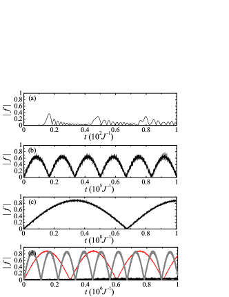
Figure 8: Time evolution of the transition amplitude for an initial symmetric polariton set at the first cavity in the case of a staggered 30-cavity array for (a) $\eta=0$, (b) $\eta=-0.25$, and (c) $\eta=-0.5$ (solid black). In (d) we show the case of a modularized CCA for $m=3$ with $J_{\mathrm{mod}}=0.1J$ (dotted red) and $m=5$ with $J_{\mathrm{mod}}=0.3J$ (thick gray). Note that $J_{\mathrm{mod}}$ was slightly increased in order to assure the formation of bi-localized states (cf. Section V). The intra-modular distortion parameter was fixed to $\eta=-0.5$. We set $g=0.01J$ and $\omega_{a}=0$ throughout. Plots are obtained from an exact diagonalization of Eq. (20) [with $\hat{H}_{\mathrm{hop}}$ being replaced with $\hat{H}_{\mathrm{mod}}$ in (d)].

Regardless of the interaction regime (single-resonance or strong coupling), the crucial factor affecting the transfer fidelity is the end-to-end localization amplitude, i.e., the occurrence of bi-localization either in the case of a standard staggered CCA or the modularized (partitioned) one. The key ingredient is thus inducing the formation of bi-localized field normal modes and tuning the atoms on resonance with those. The QST speed, however, can be managed by setting the appropriate regime and/or modularizing the CCA as in Section V.

VIII Conclusions

In this work, we addressed the problem of transferring faithfully quantum states across a CCA. We have shown that, while a staggered pattern of hopping rates offers shorter QST times with respect to a uniform pattern, a further significant reduction of the transfer time is achievable by imposing modularization on top of the staggered pattern. The modularization scheme yields up to three orders of magnitude shorter transfer times with respect to an unmodularized staggered array already for 20-site CCAs, while the gain increases for longer CCAs without affecting the performance in terms of QST fidelity.

To accomplish this task, we first focused on QST through a staggered atom-free CCA. By devising a perturbative approach to diagonalize analytically the Hamiltonian for a highly-distorted array, we showed that distortion induces the appearance of bound modes that are strongly bi-localized on the array edges. In line with QST schemes exploiting bi-localization, this allows for high-fidelity QST. As a distinctive property of the staggered configuration, though, the scaling behaviour of the fidelity as a function of the CCA size has ideal features since, for the high-distortion scenario, the fidelity is nearly insensitive to the array length (unlike in the case of a uniform bulk with weak outermost couplings). This yet comes at the cost of having relatively long transfer times. To get around this drawback, we devised a strategy based on an engineered modularization of the array into identical staggered subunits. We showed that in some paradigmatic instances this can result in a significant reduction of the transfer time while maintaining the transfer fidelity about unchanged. Despite we focused on an atom-free CCA, those findings apply to any spin chain regardless of the way it is implemented.

We then turned to a CCA where each cavity is coupled to an atom with the aim of exploring how the previous outcomes can be harnessed for transferring atomic or polaritonic states between the two array ends. In the weak-coupling regime where the atomic frequency is resonant with one of the two bi-localized field modes, QST of atomic states can be achieved in a time set by the atom-field coupling strength. For stronger atom-photon couplings, one can instead exploit the formation of pairs of bi-localized dressed states to efficiently transfer a polariton of given parity across the CCA in a time set by the energy gap between the pair of field bi-localized modes.

References

- Hartmann et al. (2008) M. J. Hartmann, F. G. S. L. Brandão, and M. B. Plenio, Laser Photon. Rev. 2, 527 (2008).
- Tomadin and Fazio (2010) A. Tomadin and R. Fazio, J. Opt. Soc. Am. B 27, A130 (2010).
- Angelakis et al. (2007) D. G. Angelakis, M. F. Santos, and S. Bose, Phys. Rev. A 76, 031805(R) (2007).
- Greentree et al. (2006) A. D. Greentree, C. Tahan, J. H. Cole, and L. C. L. Hollenberg, Nat. Phys. 2, 856 (2006).
- Hartmann et al. (2006) M. J. Hartmann, F. G. S. L. Brandão, and M. B. Plenio, Nat. Phys. 2, 849 (2006).
- Rossini and Fazio (2007) D. Rossini and R. Fazio, Phys. Rev. Lett. 99, 186401 (2007).
- Aichhorn et al. (2008) M. Aichhorn, M. Hohenadler, C. Tahan, and P. B. Littlewood, Phys. Rev. Lett. 100, 216401 (2008).
- Koch and Le Hur (2009) J. Koch and K. Le Hur, Phys. Rev. A 80, 023811 (2009).
- Schmidt and Blatter (2009) S. Schmidt and G. Blatter, Phys. Rev. Lett. 103, 086403 (2009).
- Pippan et al. (2009) P. Pippan, H. G. Evertz, and M. Hohenadler, Phys. Rev. A 80, 033612 (2009).
- Schmidt and Blatter (2010) S. Schmidt and G. Blatter, Phys. Rev. Lett. 104, 216402 (2010).
- Knap et al. (2010) M. Knap, E. Arrigoni, and W. von der Linden, Phys. Rev. B 81, 104303 (2010).
- Birnbaum et al. (2005) K. M. Birnbaum, A. Boca, R. Miller, A. D. Boozer, T. E. Northup, and H. J. Kimble, Nature 436, 87 (2005).
- Fisher et al. (1989) M. P. A. Fisher, P. B. Weichman, G. Grinstein, and D. S. Fisher, Phys. Rev. B 40, 546 (1989).
- Raftery et al. (2014) J. Raftery, D. Sadri, S. Schmidt, H. E. Türeci, and A. A. Houck, Phys. Rev. X 4, 031043 (2014).
- Kimble (2008) H. J. Kimble, Nature 453, 1023 (2008).
- Cirac et al. (1997) J. I. Cirac, P. Zoller, H. J. Kimble, and H. Mabuchi, Phys. Rev. Lett. 78, 3221 (1997).
- Serafini et al. (2006) A. Serafini, S. Mancini, and S. Bose, Phys. Rev. Lett. 96, 010503 (2006).
- Chanelière et al. (2005) T. Chanelière, D. N. Matsukevich, S. D. Jenkins, S.-Y. Lan, T. A. B. Kennedy, and A. Kuzmich, Nature 438, 833 (2005).
- Ritter et al. (2012) S. Ritter, C. Nölleke, C. Hahn, A. Reiserer, A. Neuzner, M. Uphoff, M. Mücke, E. Figueroa, J. Bochmann, and G. Rempe, Nature 484, 195 (2012).
- Bose (2003) S. Bose, Phys. Rev. Lett. 91, 207901 (2003).
- Apollaro et al. (2013) T. J. G. Apollaro, S. Lorenzo, and F. Plastina, Int. J. Mod. Phys. B 27, 1345035 (2013).
- Nohama and Roversi (2007) F. K. Nohama and J. A. Roversi, J. Mod. Opt. 54, 1139 (2007).
- Bose et al. (2007) S. Bose, D. G. Angelakis, and D. Burgarth, J. Mod. Opt. 54, 2307 (2007).
- Hu et al. (2007) F. M. Hu, L. Zhou, T. Shi, and C. P. Sun, Phys. Rev. A 76, 013819 (2007).
- Ogden et al. (2008) C. D. Ogden, E. K. Irish, and M. S. Kim, Phys. Rev. A 78, 063805 (2008).
- Makin et al. (2009) M. I. Makin, J. H. Cole, C. D. Hill, A. D. Greentree, and L. C. L. Hollenberg, Phys. Rev. A 80, 043842 (2009).
- Lu et al. (2010) J. Lu, L. Zhou, H. C. Fu, and L.-M. Kuang, Phys. Rev. A 81, 062111 (2010).
- Ciccarello (2011) F. Ciccarello, Phys. Rev. A 83, 043802 (2011).
- Dong et al. (2012) Y.-L. Dong, S.-Q. Zhu, and W.-L. You, Phys. Rev. A 85, 023833 (2012).
- Dong et al. (2013) G. Dong, Y. Zhang, M. Arshad Kamran, and B. Zou, Journal of Applied Physics 113, 143105 (2013).
- Almeida and Souza (2013) G. M. A. Almeida and A. M. C. Souza, Phys. Rev. A 87, 033804 (2013).
- Quach (2013) J. Q. Quach, Phys. Rev. A 88, 053843 (2013).
- Latmiral et al. (2015) L. Latmiral, C. Di Franco, P. L. Mennea, and M. S. Kim, Phys. Rev. A 92, 022350 (2015).
- Behzadi et al. (2013) N. Behzadi, S. K. Rudsary, and B. A. Salmas, Eur. Phys. J. D 67, 247 (2013).
- Zhou et al. (2008) L. Zhou, Z. R. Gong, Y.-x. Liu, C. P. Sun, and F. Nori, Phys. Rev. Lett. 101, 100501 (2008).
- Longo et al. (2010) P. Longo, P. Schmitteckert, and K. Busch, Phys. Rev. Lett. 104, 023602 (2010).
- Biondi et al. (2014) M. Biondi, S. Schmidt, G. Blatter, and H. E. Türeci, Phys. Rev. A 89, 025801 (2014).
- Felicetti et al. (2014) S. Felicetti, G. Romero, D. Rossini, R. Fazio, and E. Solano, Phys. Rev. A 89, 013853 (2014).
- Lombardo et al. (2014) F. Lombardo, F. Ciccarello, and G. M. Palma, Phys. Rev. A 89, 053826 (2014).
- Tiecke et al. (2014) T. G. Tiecke, J. D. Thompson, N. P. de Leon, L. R. Liu, V. Vuletić, and M. D. Lukin, Nature 508, 241 (2014).
- Christandl et al. (2004) M. Christandl, N. Datta, A. Ekert, and A. J. Landahl, Phys. Rev. Lett. 92, 187902 (2004).
- Di Franco et al. (2008) C. Di Franco, M. Paternostro, and M. S. Kim, Phys. Rev. Lett. 101, 230502 (2008).
- Plenio et al. (2004) M. B. Plenio, J. Hartley, and J. Eisert, New Journal of Physics 6, 36 (2004).
- Apollaro et al. (2012) T. J. G. Apollaro, L. Banchi, A. Cuccoli, R. Vaia, and P. Verrucchi, Phys. Rev. A 85, 052319 (2012).
- Zwick et al. (2012) A. Zwick, G. A. Álvarez, J. Stolze, and O. Osenda, Phys. Rev. A 85, 012318 (2012).
- Wójcik et al. (2005) A. Wójcik, T. Łuczak, P. Kurzyński, A. Grudka, T. Gdala, and M. Bednarska, Phys. Rev. A 72, 034303 (2005).
- Campos Venuti et al. (2007a) L. Campos Venuti, C. Degli Esposti Boschi, and M. Roncaglia, Phys. Rev. Lett. 99, 060401 (2007a).
- Plastina and Apollaro (2007) F. Plastina and T. J. G. Apollaro, Phys. Rev. Lett. 99, 177210 (2007).
- Lorenzo et al. (2013) S. Lorenzo, T. J. G. Apollaro, A. Sindona, and F. Plastina, Phys. Rev. A 87, 042313 (2013).
- Paganelli et al. (2013) S. Paganelli, S. Lorenzo, T. J. G. Apollaro, F. Plastina, and G. L. Giorgi, Phys. Rev. A 87, 062309 (2013).
- Peierls (1955) R. E. Peierls, Quantum Theory of Solids (Oxford University Press, New York, 1955).
- Huo et al. (2008) M. X. Huo, Y. Li, Z. Song, and C. P. Sun, Europhysics Letters 84, 30004 (2008).
- Kuznetsova and Zenchuk (2008) E. I. Kuznetsova and A. I. Zenchuk, Physics Letters A 372, 6134 (2008).
- Campos Venuti et al. (2007b) L. Campos Venuti, S. M. Giampaolo, F. Illuminati, and P. Zanardi, Phys. Rev. A 76, 052328 (2007b).
- Giampaolo and Illuminati (2009) S. M. Giampaolo and F. Illuminati, Phys. Rev. A 80, 050301 (2009).
- Giampaolo and Illuminati (2010) S. M. Giampaolo and F. Illuminati, New Journal of Physics 12, 025019 (2010).
- Lorenzo et al. (2015) S. Lorenzo, T. J. G. Apollaro, S. Paganelli, G. M. Palma, and F. Plastina, Phys. Rev. A 91, 042321 (2015).
- Linneweber et al. (2012) T. Linneweber, J. Stolze, and G. S. Uhrig, International Journal of Quantum Information 10, 1250029 (2012).
- Gualdi et al. (2011) G. Gualdi, S. M. Giampaolo, and F. Illuminati, Phys. Rev. Lett. 106, 050501 (2011).
- (61) G. M. A. Almeida, F. Ciccarello, T. J. G. Apollaro, and A. M. C. Souza, In preparation.
- Jaynes and Cummings (1963) E. T. Jaynes and F. W. Cummings, Proceedings of the IEEE 51, 89 (1963).