Colonization and Collapse

Abstract.

Many species live in colonies that thrive for a while and then collapse. Upon collapse very few individuals survive. The survivors start new colonies at other sites that thrive until they collapse, and so on. We introduce spatial and non-spatial stochastic processes for modeling such population dynamic. Besides testing whether dispersion helps survival in a model experiencing large fluctuations, we obtain conditions for the population to get extinct or to survive.

1. Introduction

A metapopulation model refers to populations that are spatially structured into assemblages of local populations that are connected via migrations. Each local population evolves without spatial structure; it can increase or decrease, survive, get extinct or migrate in different ways. Many biological phenomena may influence the dynamics of a metapopulation; species adopt different strategies to increase its survival probability. See Hanski [4] for more about metapopulations.

Some metapopulations (such as ants) live in colonies that thrive for a while and then collapse. Upon collapse very few individuals survive. The survivors start new colonies at other vertices that thrive until they collapse, and so on. In this paper, we introduce stochastic models to model this population dynamic and to test whether dispersion helps survival. Our non-spatial stochastic models are reminiscent of catastrophe models, see Brockwell [2]. However, instead of having the whole population living in a single colony we now have the population dispersed in a random number of colonies. We show that dispersion of the population helps survival, see Section 4. Our spatial model is similar to a contact process, see Liggett [6], in that individuals give birth to new individuals in neighboring sites. However, in our model there is no limit in the number of individuals per site. Moreover, at collapse time a site loses all its individuals at once. This introduces large fluctuations that are non standard in interacting particle systems and complicate the analysis, see Section 5.

This paper is divided into five sections. In Section 2 we define a spatial stochastic process for colonization and collapse and present some of its properties. In Section 3 the main results are established. In Section 4 we introduce a non-spatial version of our model and compare it to other models known in the literature. Finally, in Section 5 we prove the results stated in Section 3.

2. Spatial model

We denote by $\mathcal{G}=(V,E)$ a connected non-oriented graph of locally bounded degree, where $V:=V(\mathcal{G})$ is the set of vertices of $\mathcal{G}$, and $E:=E(\mathcal{G})$ is the set of edges of of $\mathcal{G}$. Vertices are considered neighbors if they belong to a common edge. The degree of a vertex $x\in V$ is the number of edges that have $x$ as an endpoint. A graph is locally bounded if all its vertices have finite degree. A graph is $k-$regular if all its vertices have degree $k.$ The distance $d(x,y)$ between vertices $x$ and $y$ is the minimal amount of edges that one must pass in order to go from $x$ to $y.$ By $\mathbb{Z}^{d}$ we denote the graph whose set of vertices is $\mathbb{Z}^{d}$ and the set of edges is $\{\left\langle(x_{1},\ldots,x_{d}),(y_{1},\ldots,y_{d})\right\rangle:|x_{1}-y_{1}|+\ldots|x_{d}-y_{d}|=1\}.$ Besides, by $\mathbb{T}^{d}$, $d\geq 2$, we denote the degree $d+1$ homogeneous tree.

At any time each vertex of ${\mathcal{G}}$ may be either occupied by a colony or empty. Each colony is started by a single individual. The number of individuals in each colony behaves as a Yule process (i.e. pure birth) with birth rate $\lambda\geq 0$. To each vertex is associated a Poisson process with rate 1 in such a way that when the exponential time occurs at a vertex occupied by a colony, that colony collapses and its vertex becomes empty. At the time of collapse each individual in the colony survives with a (presumably small) probability $p\in(0,1)$ or dies with probability $1-p$. Each individual that survives tries to found a new colony on one of the nearest neighbor vertices by first picking a vertex at random. If the chosen vertex is occupied, that individual dies, otherwise the individual founds there a new colony. We denote by $CC(\mathcal{G},\lambda,p)$ the Colonization and Collapse model.

The $CC(\mathcal{G},\lambda,p)$ is a continuous time Markov process whose state space is $\mathbb{N}^{V}$ and whose evolution (status at time $t$) is denoted by $\eta_{t}$. For a vertex $x\in V$, $\eta_{t}(x)=i$ means that at the time $t$ there are $i$ individuals at the vertex $x$. We consider $|\eta_{t}|=\sum_{x\in V}\eta_{t}(x)$.

Definition 2.1.

Let $\eta_{t}$ be a $CC(\mathcal{G},\lambda,p)$, starting with a finite number of colonies. If $\mathbb{P}(|\eta_{t}|\geq 1\text{ for all }t\geq 0)>0$ we say that $\eta_{t}$ survives (globally). Otherwise, we say that $\eta_{t}$ dies out (globally).

Remark 2.2.

If the process $\eta_{t}$ starts from an infinite number of colonies, then $\mathbb{P}(|\eta_{t}|\geq 1\text{ for all }t\geq 0)=1,$ which means that $\eta_{t}$ survives with probability 1. Still we can see local death according to the following definition.

Definition 2.3.

Let $\eta_{t}$ be a $CC(\mathcal{G},\lambda,p).$ We say that $\eta_{t}$ dies locally if for any vertex $x\in V$ there is a finite random time $T$ such that $\eta_{t}(x)=0$ for all $t>T$. Otherwise we say that $\eta_{t}$ survives locally.

Remark 2.4.

Local death corresponds to a finite number of colonizations for every vertex. It is clear that global death implies local death but the opposite is not always truth. As an example consider $\eta_{t}$ a $CC(\mathbb{Z}^{3},0,1)$ with $|\eta_{0}|=1$. In this case $\eta_{t}$ can be seen as a symmetric random walk on $\mathbb{Z}^{3}$, therefore transient, which implies that $\eta_{t}$ dies locally but survives globally.

By coupling arguments one can see that $\mathbb{P}(|\eta_{t}|\geq 1\text{ for all }t\geq 0)$ is a non-decreasing function of $\lambda$ and also of $p$. So we define

$$\lambda_{c}(p,\mathcal{G}):=\inf\{\lambda:\mathbb{P}^{\delta_{x}}(|\eta_{t}|\geq 1\text{ for all }t\geq 0)>0\},$$

where $x$ is a fixed vertex, and $\mathbb{P}^{\delta_{x}}$ is the law of the process $\eta_{t}$ starting with one colony at $x$. The function $\lambda_{c}(p,\mathcal{G})$ is non-increasing on $p$. Moreover, $\lambda_{c}(1,\mathcal{G})=0$ and $\lambda_{c}(0,\mathcal{G})=\infty$.

Definition 2.5.

Let $\eta_{t}$ be a $CC(\mathcal{G},\lambda,p)$ with $0<p<1$. We say that $\eta_{t}$ exhibits phase transition (on $\lambda$) if $0<\lambda_{c}(p,\mathcal{G})<\infty.$

Remark 2.6.

Using coupling arguments, we can construct $\eta_{t}$ and $\hat{\eta}_{t}$ be two copies of $CC(\mathcal{G},\lambda,p)$ such that $\eta_{t}\leq\hat{\eta}_{t}$ for all times $t>0$, provided that $\eta_{0}\leq\hat{\eta}_{0}$. This monotonic property implies that if $\eta_{t}$ survives, $\hat{\eta}_{t}$ also does. Moreover, if $\hat{\eta}_{t}$ dies out (or dies locally) then $\eta_{t}$ does too.

Observe that, as the number of individuals per vertex is not bounded, it is conceivable that the process survives on a finite graph. Next we show that it does not happen.

Proposition 2.7.

For any finite graph and starting from any initial configuratiion, the colonization and collapse process dies out.

Proof.

Let $\alpha$ be the probability at a colony collapse time, zero individuals attempts to found new colonies at neighboring vertices.

From the fact that the probability that a Yule process, starting from one individual, has $j$ individuals at time $t$ is $e^{-\lambda t}(1-e^{-\lambda t})^{j-1},$ we have that

$$\alpha=\int_{0}^{\infty}e^{-t}\sum_{j=1}^{\infty}e^{-\lambda t}(1-e^{-\lambda t})^{j-1}(1-p)^{j}dt.$$

Let $n$ and $m$ be the number of vertices of $\mathcal{G}$ and its maximum degree, respectively. In order to show sufficient conditions for extinction we couple the number of colonies in the original model to $X_{t}$, the following continuous time branching process. Each individual is independently associated to an exponential random variable of rate 1 in such a way that, when its exponential time occurs, it dies with probability $\alpha$ or is replaced by $m$ individuals with probability $1-\alpha$. We also consider a restriction that makes the total number of individuals always smaller or equal than $n$ by suppressing the births that would make $X_{t}$ larger than $n$.

Let $C_{t}$ be the number of colonies at time $t$ in the colonization and collapse process. At time $t=0$ let $X_{0}=C_{0}$. Moreover, we couple each individual in $X_{0}$ to a colony in the colonization and collapse process by using the same exponential random variable of rate 1. When an exponential occurs there are two possibilities. With probability $\alpha$ both $X_{t}$ and $C_{t}$ decrease by 1. With probability $1-\alpha$ the process $X_{t}$ grows by $m-1$ individuals and $C_{t}$ grows by at most $m-1$ colonies. This is so because in the colonization process we have spatial constraints and attempted colonizations only occur at vertices that are empty. Hence, new colonies correspond to births for $X_{t}$. We couple each new colony to a new individual in $X_{t}$ by using the same mean 1 exponential random variable. This coupling yields for all $t\geq 0$

$$X_{t}\geq C_{t}.$$

Note now that $\alpha>0$ and that $X_{t}$ is a finite Markov process with an absorbing state. Hence, $X_{t}$ dies out with probability 1. So does $C_{t}$ and therefore the colonization and collapse process. ∎

3. Main Results

Next, we show sufficient conditions for global extinction and local extinction for the colonization and collapse process on infinite graphs.

Theorem 3.1.

Let $\mathcal{G}$ be a $m$-regular graph, $\eta_{t}$ a $CC(\mathcal{G},\lambda,p)$ and

$$\mu(m)=m-\frac{m}{\lambda}\sum_{k\geq 1}B\left(1+\frac{1}{\lambda},k\right)\left(1-\frac{p}{m}\right)^{k},$$

where $B(a,b)=\int_{0}^{1}u^{a-1}(1-u)^{b-1}du$ is the beta function.

• If $\mu(m)\leq 1$ and $|\eta_{0}|<\infty$, then $\eta_{t}$ dies out locally and globally.

• Let $\mathcal{G}=\mathbb{Z}^{d},\ d\geq 1.$ If $\mu(2d)<1$ and $\eta_{0}(x)\leq 1$ for every $x$ in $\mathbb{Z}^{d}$ then $\eta_{t}$ dies locally.

• Let $\mathcal{G}=\mathbb{T}^{d},\ d\geq 1.$ If $\mu(d+1)<1/d$ and $\eta_{0}(x)\leq 1$ for every $x$ in $\mathbb{T}^{d}$ then $\eta_{t}$ dies locally.

Remark 3.2.

Observe that for all $m\geq 1$ and $\lambda$ fixed, there exists $p>0$ such that $\mu(m)\leq 1$. Furthermore, $\mu(m)$ can be expressed in terms of the Gauss hypergeometric function ${{}_{2}F_{1}}$ (see Luke [8]),

$$\mu(m)=m-\frac{m-p}{\lambda+1}{{}_{2}F_{1}}\left(1,1;2+\frac{1}{\lambda};1-\frac{p}{m}\right).$$

Next, we show sufficient conditions for survival for colonization and collapse process on some infinite graphs.

Theorem 3.3.

For $p>0$ and $\lambda:=\lambda(p,\mathcal{G})>0$ large enough, the $CC(\mathcal{G},\lambda,p)$ with $\mathcal{G}=\mathbb{Z}^{d}$ or $\mathbb{T}^{d}$ survives globally and locally.

Remark 3.4.

From Theorems 3.1 and 3.3 it follows that for $\mathcal{G}=\mathbb{Z}^{d}$ or $\mathbb{T}^{d}$ and $p\in(0,1)$, there exists phase transition (on $\lambda$) for $CC(\mathcal{G},\lambda,p).$ So, there exists a function $\lambda_{c}(\cdot,\mathcal{G}):(0,1)\rightarrow\mathbb{R}^{+}$ such that the survival and extinction regime for $CC(\mathcal{G},\lambda,p)$ can be represented as in Figure 3.1.

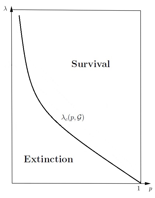
Figure 3.1. Phase transition to $CC(\mathcal{G},\lambda,p),$ with $\mathcal{G}=\mathbb{Z}^{d}\ (\text{or}\ \mathbb{T}^{d}).$

4. Non spatial models

So called Catastrophe Models have been studied extensively and are quite close to our model, see Kapodistria et al. [5] for references on the subject. Particularly relevant is the birth and death process with binomial catastrophes, see Example 2 in Brockwell [2]. We now describe this model. It is a single colony model. Each individual gives birth at rate $\lambda>0$ and dies at rate $\mu>0$. Moreover, catastrophes (i.e. collapses) happen at rate $a>0$. When a catastrophe happens every individual in the colony has a probability $p$ of surviving and $1-p$ of dying, independently of each other. Brockwell [2] has shown that survival (i.e. at all times there is at least one individual in the colony) has positive probability if and only if $\lambda>\mu$ and

$$\mu-a\log p<\lambda.$$

Hence, there is a critical value for $p$,

$$p_{1}=\exp(-\frac{\lambda-\mu}{a}).$$

The single colony model survives if and only if $p>p_{1}$.

Next we introduce a non spatial version of our model and compare it to the catastrophe model above. Consider a model for which every individual gives birth at rate $\lambda$ and dies at rate $\mu$. We start with a single individual and hence with a single colony. When a colony collapses individuals in the colony survive with probability $p$ and die with probability $1-p$ independently of each other. Every surviving individual founds a new colony which eventually collapses. Colonies collapse independently of each other at rate $a>0$. The proof in Schinazi [9] may be adapted to show that survival has positive probability if and only if

$$pE\left[\exp\left((\lambda-\mu)T\right)\right]>1,$$

where $T$ has a rate $a$ exponential distribution. It is easy to see that if $\lambda\geq\mu+a$ then the expected value on the l.h.s. is $+\infty$ and the inequality holds for any $p>0$. It is also easy to see that the inequality cannot hold if $\lambda\leq\mu$. Hence, from now on we assume that $\mu<\lambda<\mu+a.$ After computing the expected value and solving for $p$ we get that survival is possible if and only if

$$p>1-\frac{\lambda-\mu}{a}.$$

That is, when $\mu<\lambda<\mu+a$ the model with multiple colonies has a critical value

$$p_{2}=1-\frac{\lambda-\mu}{a}.$$

The multiple colonies model survives if and only if $p>p_{2}$.

Since $\exp(-x)>1-x$ for all $x\not=0$ we have that $p_{1}>p_{2}$ for any $\lambda>\mu$. Hence, it is easier for the model with multiple colonies to survive than it is for the model with a single colony. That is, living in multiple smaller colonies is a better survival strategy than living in a single big colony. Note that this conclusion was not obvious. The one colony model has a catastrophe rate of $a$ while the multiple colonies model has a catastrophe rate of $na$ if there are $n$ colonies. Moreover, a catastrophe is more likely to wipe out a smaller colony than a larger one. On the other hand multiple colonies give multiple chances for survival and this turns out to be a critical advantage of the multiple colonies model over the single colony model.

5. proofs

5.1. Auxiliary results

For $\eta_{t}$ being a $CC(\mathcal{G},\lambda,p)$ process, we know that some colonization attempts will not succeed because the vertex on which the attempted colonization takes place is already occupied. This creates dependence between the number of new colonies created upon the collapse of different colonies. Because of this lack of independence, explicit probability computation seems impossible. In order to prove Theorem 3.1, we introduce a branching-like process which dominates $\eta_{t}$, in a certain sense, and for which explicit computations are possible. This process is denoted by $\xi_{t}$ and defined as follows.

Auxiliary process $\xi_{t}$ :
Each vertex of $\mathcal{G}$ might be empty or occupied by a number of colonies. Each colony starts from a single individual. The number of individuals in a colony at time $t$ is determined by a pure birth process of rate $\lambda$. Each colony is associated to a mean 1 exponential random variable. When the exponential clock rings for a colony it collapses and each individual, independently from everything else, survives with probability $p>0$ or dies with probability $1-p$. Each individual who survives tries to create a new colony at one of the nearest neighbor vertices picked at random. At every neighboring vertex we allow at most one new colony to be created. Hence, in the process $\xi_{t}$ when a colony placed at vertex $x$ collapses, it is replaced by 0,1,.., or degree$(x)$ new colonies, each new colony on a distinct neighboring site of $x$.

Observe that birth and collapse rates are the same for colonies in $\xi_{t}$ and $\eta_{t}$. To each colony created in process $\eta_{t}$ corresponds a colony created in the process $\xi_{t}$. But not every colony created in the process $\xi_{t}$ has its correspondent in the process $\eta_{t}$. Techniques such as in Liggett [6, Theorem 1.5 in chapter III] can be used to construct the processes $\xi_{t}$ and $\eta_{t}$ in the same probability space in such a way that, if they start with the same initial configuration, if there is a colony of size $i$ on a vertex $x$ for $\eta_{t}$ then there is at least one colony of size $i$ for $\xi_{t}$ on the same vertex $x$.

Lemma 5.1.

Let $\mathcal{G}$ be a $m-$regular graph and $W_{m}(\lambda,p)$ the number of new colonies created by individuals of a collapsing colony in the process $\xi_{t}$ on $\mathcal{G}$. Then

• $\mu(m):=\mathbb{E}[W_{m}(\lambda,p)]=m-\frac{m}{\lambda}\sum_{k\geq 1}B\left(1+\frac{1}{\lambda},k\right)\left(1-\frac{p}{m}\right)^{k}.$

• $q_{\lambda}:=\mathbb{P}[W_{m}(\lambda,p)=m]\rightarrow 1$ as $\lambda\rightarrow\infty.$

Remark 5.2.

Observe that for the process $\eta_{t}$ the probability that upon a collapse at vertex $x$ each one of its $m$ neighbors gets at least one colonization attempt is equal to $q_{\lambda}$.

Proof of Lemma 5.1.

$(i)$ Consider a colony at some vertex $x$ of $\mathcal{G}$. Let $Y$ be the number of individuals in the colony at collapse time. Then

$$\mathbb{P}[Y=k]=\int_{0}^{\infty}e^{-t}e^{-\lambda t}(1-e^{-\lambda t})^{k-1}dt=\frac{1}{\lambda}B\left(1+\frac{1}{\lambda},k\right),$$ (5.1)

where the last equality is obtained by the substitution $u=e^{-\lambda t}$ and the definition of the beta function.

Enumerate each neighbor of vertex $x$ from 1 to $m$, then $W_{m}(\lambda,p)=\sum_{i=1}^{m}I_{i},$ where $I_{i}$ is the indicator function of the event {A new colony is created in the $i-$th neighbor of $x$.}. Hence,

$$\mathbb{E}[W_{m}(\lambda,p)]=\sum_{i=1}^{m}\mathbb{P}[I_{i}=1]=m\mathbb{P}[I_{1}=1].$$ (5.2)

Observe that

$$\mathbb{P}[I_{1}=1|Y=k]=1-\left(1-\frac{p}{m}\right)^{k}.$$

Therefore,

$$\mathbb{P}[I_{1}=1] = \sum_{k=1}^{\infty}\left[1-\left(1-\frac{p}{m}\right)^{k}\right]\mathbb{P}[Y=k]$$ (5.3)

$$= 1-\frac{1}{\lambda}\sum_{k=1}^{\infty}\left(1-\frac{p}{m}\right)^{k}B\left(1+\frac{1}{\lambda},k\right)$$

where the last equality is obtained by (5.1). Substituting (5.3) in (5.2) we obtain the desired result.

$(ii)$ Observe that

$$\mathbb{P}[W_{m}(\lambda,p)=m] = \mathbb{P}[I_{1}=1,\ldots,I_{m}=1]$$ (5.4)

$$= 1-\mathbb{P}[I_{i}=0\text{ for some }i\in{1,\ldots m}]$$

$$\geq 1-\sum_{i=1}^{m}\mathbb{P}[I_{i}=0]$$

$$= 1-m\mathbb{P}[I_{1}=0]$$

$$= 1-\frac{m}{\lambda}\sum_{k=1}^{\infty}\left(1-\frac{p}{m}\right)^{k}B\left(1+\frac{1}{\lambda},k\right)$$

$$\geq 1-\frac{m}{\lambda}\sum_{k=1}^{\infty}\left(1-\frac{p}{m}\right)^{k}B\left(1,k\right)$$

Letting $\lambda\rightarrow\infty$ in (5.4) we obtain the result.

∎

5.2. Proofs of main results

Proof of Theorem 3.1 (i).

Consider $\xi_{t}$ starting with one colony at the origin and let $Z_{0}=1.$ This colony we call the $0$-th generation. Upon collapse of that colony a random number of new colonies are created. Denote this random number by $Z_{1}$. These are the first generation colonies. Every first generation colony gives birth (at different random times) to a random number of new colonies. These new colonies are the second generation colonies and their total number is denoted by $Z_{2}$. More generally, let $n\geq 1$, if $Z_{n-1}=0$ then $Z_{n}=0$, if $Z_{n-1}\geq 1$ then $Z_{n}$ is the total number of colonies created by the previous generation colonies.

We claim that $Z_{n}$, $n=0,1,\dots$ is a Galton-Watson process. This is so because the offsprings of different colonies in the process $\xi_{t}$ have the same distribution and are independent.

The process $Z_{n}$ dies out if and only if $\mathbb{E}[Z_{1}]\leq 1$. From Lemma 5.1$.(i)$ we know that $\mathbb{E}[Z_{1}]=\mu(m).$

Observe that if the process $Z_{n}$ dies out, the same happens to $\xi_{t}$ and hence to $\eta_{t}$. It is easy to see that the proof works if the process starts from any finite number of colonies. ∎

Proof of Theorem 3.1 (ii).

From the monotonic property of $\eta_{t}$ it suffices to show local extinction for the process starting with one individual at each vertex of $\mathbb{Z}^{d}$. We will actually prove local extinction for the process $\xi_{t}$ starting with one individual at each vertex of $\mathbb{Z}^{d}.$

Fix a vertex $x$. If at time $t$ there exists a colony at vertex $x$ (for the process $\xi_{t}$) then it must descend from a colony present at time $0$. Assume that the colony at $x$ descends from a colony at some site $y$. Let $Z_{n}(y)$ be the number of colonies at the $n$-th generation of the colony that started at $y$. The process $Z_{n}(y)$ has the same distribution as the process $Z_{n}$ defined above. In order for a descendent of $y$ to eventually reach $x$ the process $Z_{n}(y)$ must have survived for at least $d(x,y)$ generations. This is so because each generation gives birth only on nearest neighbors vertices. The process $Z_{n}(y)$ is a Galton-Watson process with $Z_{0}(y)=1$ and mean offspring $\mu=\mu(2d).$

Let $n=d(x,y)$, then

$$\mathbb{P}(Z_{n}(y)\geq 1)\leq\mathbb{E}(Z_{n}(y))=\mu^{n}=\mu^{d(x,y)}$$

and

$$\sum_{y\in\mathbb{Z}^{d}}\mathbb{P}(Z_{n}(y)\geq 1)\leq\sum_{y\in\mathbb{Z}^{d}}\mu^{d(x,y)}=$$

$$\sum_{n\geq 1}\#\{x\in\mathbb{Z}^{d}:d(x,y)=n\}\ \mu^{n}=\sum_{n\geq 1}{n+d-1\choose n}\mu^{n}<\infty,$$

for $\mu<1$.

The Borel-Cantelli lemma shows that almost surely there are only finitely many $y$’s such that descendents from $y$ eventually reach $x$. From $(i)$ we know that a process starting from a finite number of individuals dies out almost surely. Hence, after a finite random time there will be no colony at vertex $x$. ∎

Proof of Theorem 3.1 (iii).

The proof is analogous to $(ii)$. In this case, $\mu=\mu(d+1)$ and

$$\sum_{y\in\mathbb{T}^{d}}\mu^{d(x,y)}=\sum_{n\geq 1}(d+1)d^{n-1}\mu^{n}<\infty,$$

for $\mu<1/d$. ∎

Proof of Theorem 3.3:.

We first give the proof on the one dimensional lattice $\mathbb{Z}$.

We start by giving an informal construction of the process. We put a Poisson process with rate 1 at every site of $\mathbb{Z}$. All the Poisson processes are independent. At the Poisson process jump times the colony at the site collapses if there is a colony. If not, nothing happens. We start the process with finitely many colonies. Each colony starts with a single individual and is associated to a Yule process with birth rate $\lambda$. At collapse time, given that the colony at site $x$ has $n$ individuals we have a binomial random variable with parameters $(n,p)$. The binomial gives the number $k$ of potential survivors. If $k\geq 1$ then each survivor attempts to found a new colony on $x+1$ with probability $\frac{1}{2}$ or on $x-1$ also with probability $\frac{1}{2}$. The attempt succeeds on an empty site. We associate a new Yule process to a new colony, independently of everything else.

We use the block construction presented in Bramson and Durrett [1]. First some notation. For integers $m$ and $n$ we define

$$I=[-L,L]\qquad I_{m}=2mL+I,$$

$$B=(-4L,4L)\times[0,T]\qquad B_{m,n}=(2mL,nT)+B,$$

where

$$T=\frac{5}{2}L$$

and

$$\mathbb{L}=\left\{(m,n)\in\mathbb{Z}^{2}:m+n\mbox{ is even}\right\}.$$

We say that the interval $I_{m}$ is half-full if at least every other site of $I_{m}$ is occupied. That is, the gap between two occupied sites in $I_{m}$ is at most one site.

We declare $(m,n)\in\mathbb{L}$ wet if starting with $I_{m}$ half-full at time $nT$ then $I_{m-1}$ and $I_{m+1}$ are also half-full at time $(n+1)T$. Moreover, we want the last event to happen using only the Poisson and Yule processes inside the box $B_{m,n}$. That is, we consider the process restricted to $B_{m,n}$.

We are going to show that for any $\epsilon>0$ there are $\lambda$, $L$ and $T$ so that for any $(m,n)\in\mathbb{L}$

$$P((m,n)\mbox{ is wet})\geq 1-\epsilon.$$

By translation invariance it is enough to prove this for $(m,n)=(0,0)$. The proof has two steps.

$\bullet$ Let $E$ be the event that every collapse in the finite space-time box $B$ is followed by at least one attempted colonization on the left and one on the right of the collapsed site. We claim that for every $\epsilon>0$, we can pick $L$, $T$ and $\lambda>0$ large enough so that $P(E)\geq 1-\epsilon.$ We now give the outline of why this is true. Since collapse times are given by rate one Poisson processes on each site of $B$ the total number of collapses inside $B$ is bounded above by a Poisson distribution with rate $(8L+1)T$. Hence, with high probability there are less than $2(8L+1)T$ collapses inside $B$ for $L$ large enough. We also take $\lambda$ large enough so that at every collapsing time the colony will have so many individuals that attempted colonizations to the left and right will be almost certain (see Lemma 5.1$.(ii)$). Since the number of collapses can be bounded with high probability the probability of the event $E$ can be made arbitrarily close to 1.

$\bullet$ At time 0 we start the process with the interval $I$ half-full. Let $r_{t}$ and $\ell_{t}$ be respectively the leftmost and rightmost occupied sites at time $t\geq 0$. Conditioned on the event $E$ it is easy to see that the interval $[\ell_{t},r_{t}]$ is half-full at any time $t\leq T$. Observe also that conditioned on $E$, every time there is a collapse at $r_{t}$ then $r_{t}$ jumps to $r_{t}+1$. Since the number of collapses at $r_{t}$ is a Poisson process with rate 1 we have that $\frac{r_{t}}{t}$ converges to 1. Hence, for $T=\frac{5}{2}L$ we have that $r_{T}$ belongs to $(3L,4L)$ with a probability arbitrarily close to 1 provided $L$ is large enough. A symmetric argument shows that $\ell_{T}$ belongs to $(-4L,-3L)$. Since the interval $[\ell_{T},r_{T}]$ contains $I_{-1}$ and $I_{1}$, both of these intervals are half-full. Hence, for any $\epsilon>0$ we can pick $L$ and $\lambda$ large enough so that $P((0,0))\mbox{ is wet})\geq 1-\epsilon.$

The preceding construction gives a coupling between our colonization and collapse model and an oriented percolation model on $\mathbb{L}$. The oriented percolation model is 1-dependent and it is well known that for $\epsilon>0$ small enough $(0,0)$ will be in an infinite wet cluster which contains infinitely many vertices like $(0,2n)$, see Durrett [3]. That fact corresponds, by the coupling, to local survival in the colonization and collapse model. Note that the proof was done for the process restricted to the boxes $B_{m,n}$. However, if this model survives then so does the unrestricted model. This is so because the model is attractive and more births can only help survival.

Consider now $\mathbb{Z}^{d}$ with $d\geq 2$. First observe that from the case $d=1$ we have a sufficient condition for local survival for the process restricted to a fixed line of $\mathbb{Z}^{d}$. Since the model is attractive this is enough to show local survival on $\mathbb{Z}^{d}$. This is so because the unrestricted model will bring more births (but not more deaths) to the sites on the fixed line.

For $\mathbb{T}^{d}$ the local survival follows analogously as in $\mathbb{Z}^{d}$, observing that $\mathbb{Z}$ is embedded in $\mathbb{T}^{d}$. ∎

Remark 5.3.

Our argument shows that both critical values, $\lambda_{c}(p,\mathbb{Z}^{d})$ and $\lambda_{c}(p,\mathbb{T}^{d})$, decrease with $d$. The more difficult issue is whether the critical value is strictly decreasing. We conjecture it is but this is a hard question even for the contact process, see Liggett [7].

References

- [1] M. Bramson and R. Durrett Simple proof of the stability criterion of Gray and Griffeath. Probability Theory and Related Fields 80, 293-298. (1988).
- [2] P.J. Brockwell. The extinction time for a general birth and death process with catastrophes. Journal of Applied Probability 23, 851-858. (1986).
- [3] R. Durrett. Oriented Percolation in two dimensions. The Annals of Probability. 12 (4), 999-1040. (1984).
- [4] I. Hanski Metapopulation Ecology. Oxford Univ. Press, Oxford. (1999).
- [5] S. Kapodistria, T. Phung-Duc and J. Resing. Linear birth/immigration-death process with binomial catastrophes. Probability in the Engineering and Informational Sciences 30 (1), 79-111 (2016).
- [6] T. Liggett. Interacting particle systems. Springer-Verlag. (1985).
- [7] T. Liggett. Stochastic Interacting Systems: Contact, Voter and Exclusion Processes. Springer, New York. (1999).
- [8] Y.L. Luke. The Special Functions and Their Approximations. Academic Press, New York. vol. 1. (1969)
- [9] R. Schinazi. Does random dispersion help survival? Journal of Statistical Physics, 159 (1),101-107. (2015).