Incompressible Limit of Solutions of Multidimensional Steady Compressible Euler Equations

Abstract.

A compactness framework is formulated for the incompressible limit of approximate solutions with weak uniform bounds with respect to the adiabatic exponent for the steady Euler equations for compressible fluids in any dimension. One of our main observations is that the compactness can be achieved by using only natural weak estimates for the mass conservation and the vorticity. Another observation is that the incompressibility of the limit for the homentropic Euler flow is directly from the continuity equation, while the incompressibility of the limit for the full Euler flow is from a combination of all the Euler equations. As direct applications of the compactness framework, we establish two incompressible limit theorems for multidimensional steady Euler flows through infinitely long nozzles, which lead to two new existence theorems for the corresponding problems for multidimensional steady incompressible Euler equations.

1. Introduction

We are concerned with the incompressible limit of solutions of multidimensional steady compressible Euler equations. The steady compressible full Euler equations take the form:

$$\begin{cases}\mbox{div}\,(\rho u)=0,\\ \mbox{div}\,(\rho u\otimes u)+\nabla p=0,\\ \mbox{div}\,(\rho uE+up)=0,\end{cases}$$ (1.1)

while the steady homentropic Euler equations have the form:

$$\begin{cases}\mbox{div}\,(\rho u)=0,\\[2.84526pt] \mbox{div}\,(\rho u\otimes u)+\nabla p=0,\end{cases}$$ (1.2)

where $x:=(x_{1},\cdots,x_{n})\in\mathbb{R}^{n}$ with $n\geq 2$, $u:=(u_{1},\cdots,u_{n})\in\mathbb{R}^{n}$ is the flow velocity,

$$|u|=\Big{(}\sum_{i=1}^{n}u_{i}^{2}\Big{)}^{1/2}$$ (1.3)

is the flow speed, $\rho$, $p$, and $E$ represent the density, pressure, and total energy respectively, and $u\otimes u:=(u_{i}u_{j})_{n\times n}$ is an $n\times n$ matrix.

For the full Euler case, the total energy is

$$E=\frac{|u|^{2}}{2}+\frac{p}{(\gamma-1)\rho},$$ (1.4)

with adiabatic exponent $\gamma>1$, the local sonic speed is

$$c=\sqrt{\frac{\gamma p}{\rho}},$$ (1.5)

and the Mach number is

$$M=\frac{|u|}{c}=\frac{1}{\sqrt{\gamma}}\,|u|\sqrt{\frac{\rho}{p}}.$$ (1.6)

For the homentropic case, the pressure-density relation is

$$p=\rho^{\gamma},\qquad\gamma>1.$$ (1.7)

The local sonic speed is

$$c=\sqrt{\gamma\rho^{\gamma-1}}=\sqrt{\gamma}\,p^{\frac{\gamma-1}{2\gamma}},$$ (1.8)

and the Mach number is defined as

$$M=\frac{|u|}{c}=\frac{1}{\sqrt{\gamma}}\,|u|p^{\frac{1-\gamma}{2\gamma}}.$$ (1.9)

The incompressible limit is one of the fundamental fluid dynamic limits in fluid mechanics. Formally, the steady compressible full Euler equations (1.1) converge to the steady inhomogeneous incompressible Euler equations:

$$\begin{cases}\mbox{div}\,u=0,\\ \mbox{div}\,(\rho u)=0,\\ \mbox{div}\,(\rho u\otimes u)+\nabla p=0,\end{cases}$$ (1.10)

while the homentropic Euler equations (1.2) converge to the steady homogeneous incompressible Euler equations:

$$\begin{cases}\mbox{div}\,u=0,\\[2.84526pt] \mbox{div}\,(u\otimes u)+\nabla p=0.\end{cases}$$ (1.11)

However, the rigorous justification of this limit for weak solutions has been a challenging mathematical problem, since it is a singular limit for which singular phenomena usually occur in the limit process. In particular, both the uniform estimates and the convergence of the nonlinear terms in the incompressible models are usually difficult to obtain. Moreover, tracing the boundary conditions of the solutions in the limit process is a tricky problem.

Generally speaking, there are two processes for the incompressible limit: The adiabatic exponent $\gamma$ tending to infinity, and the Mach number $M$ tending to zero [22, 23]. The latter is also called the low Mach number limit. A general framework for the low Mach number limit for local smooth solutions for compressible flow was established in Klainerman-Majda [16, 17]. In particular, the incompressible limit of local smooth solutions of the Euler equations for compressible fluids was established with well-prepared initial data i.e., the limiting velocity satisfies the incompressible condition initially, in the whole space or torus. Indeed, by analyzing the rescaled linear group generated by the penalty operator (cf. [27]), the low Mach number limit can also be verified for the case of general data, for which the velocity in the incompressible fluid is the limit of the Leray projection of the velocity in the compressible fluids. This method also applies to global weak solutions of the isentropic Navier-Stokes equations with general initial data and various boundary conditions [10, 11, 20]. In particular, in [20], the incompressible limit on the stationary Navier-Stokes equations with the Dirichlet boundary condition was also shown, in which the gradient estimate on the velocity played the major role. For the one-dimensional Euler equations, the low Mach number limit has been proved by using the $BV$ space in [3]. For the limit $\gamma\rightarrow\infty$, it was shown in [21] that the compressible isentropic Navier-Stokes flow would converge to the homogeneous incompressible Navier-Stokes flow. Later, the similar limit from the Korteweg barotropic Navier-Stokes model to the homogeneous incompressible Navier-Stokes model was also considered in [18].

For the steady flow, the uniqueness of weak solutions of the steady incompressible Euler equations is still an open issue. Thus, the incompressible limit of the steady Euler equations becomes more fundamental mathematically; it may serve as a selection principle of physical relevant solutions for the steady incompressible Euler equations since a weak solution should not be regarded as the compressible perturbation of the steady incompressible Euler flow in general. Furthermore, for the general domain, it is quite challenging to obtain directly a uniform estimate for the Leray projection of the velocity in the compressible fluids.

In this paper, we formulate a suitable compactness framework for weak solutions with weak uniform bounds with respect to the adiabatic exponent $\gamma$ by employing the weak convergence argument. One of our main observations is that the compactness can be achieved by using only natural weak estimates for the mass conservation and the vorticity, which was introduced in [7, 15]. Another observation is that the incompressibility of the limit for the homentropic Euler flow follows directly from the continuity equation, while the incompressibility of the limit for the full Euler flow is from a combination of all the Euler equations. Finally, we find a suitable framework to satisfy the boundary condition without the strong gradient estimates on the velocity. As direct applications of the compactness framework, we establish two incompressible limit theorems for multidimensional steady Euler flows through infinitely long nozzles. As a consequence, we can establish the new existence theorems for the corresponding problems for multidimensional steady incompressible Euler equations.

The rest of this paper is organized as follows. In §2, we establish the compactness framework for the incompressible limit of approximate solutions of the steady full Euler equations and the homentropic Euler equations in $\mathbb{R}^{n}$ with $n\geq 2$. In §3, we give a direct application of the compactness framework to the full Euler flow through infinitely long nozzles in $\mathbb{R}^{2}$. In §4, the incompressible limit of homentropic Euler flows in the three-dimensional infinitely long axisymmetric nozzle is established.

2. Compactness Framework for Approximate Steady Euler Flows

In this section, we establish the compensated compactness framework for approximate solutions of the steady Euler equations in $\mathbb{R}^{n}$ with $n\geq 2$. We first consider the homentropic case, that is, the approximate solutions $(u^{(\gamma)},p^{(\gamma)})$ satisfy

$$\begin{cases}\mbox{div}\big{(}\rho^{(\gamma)}u^{(\gamma)}\big{)}=e_{1}(\gamma),\\[2.84526pt] \mbox{div}\big{(}\rho^{(\gamma)}u^{(\gamma)}\otimes u^{(\gamma)}\big{)}+\nabla p^{(\gamma)}=e_{2}(\gamma),\end{cases}$$ (2.1)

where $e_{1}(\gamma)$ and $e_{2}(\gamma):=(e_{21}(\gamma),\cdots,e_{2n}(\gamma))^{\top}$ are sequences of distributional functions depending on the parameter $\gamma$.

Remark 2.1.

The distributional functions $e_{i}(\gamma)$, $i=1,2$, here present possible error terms from different types of approximation. If $(u^{(\gamma)},p^{(\gamma)})$ with $\rho^{(\gamma)}:=\big{(}p^{(\gamma)}\big{)}^{\frac{1}{\gamma}}$ are the exact solutions of the steady Euler flows, $e_{i}(\gamma),i=1,2$, are both equal to zero. Moreover, the same remark is true for the full Euler case, where $e_{i}(\gamma),i=1,2,3$, are the distributional functions as introduced in (2.17).

Let the sequences of functions $u^{(\gamma)}(x):=(u^{(\gamma)}_{1},\cdots,u^{(\gamma)}_{n})(x)$ and $p^{(\gamma)}(x)$ be defined on an open bounded subset $\Omega\subset\mathbb{R}^{n}$ such that the following qualities:

$$\rho^{(\gamma)}:=(p^{(\gamma)})^{\frac{1}{\gamma}},\quad|u^{(\gamma)}|:=\sqrt{\sum_{i=1}^{n}(u_{i}^{(\gamma)})^{2}},\quad c^{(\gamma)}:=\sqrt{\gamma}\big{(}p^{(\gamma)}\big{)}^{\frac{\gamma-1}{2\gamma}},\quad M^{(\gamma)}:=\frac{|u^{(\gamma)}|}{c^{(\gamma)}},$$ (2.2)

$$E^{(\gamma)}=\frac{|u^{(\gamma)}|^{2}}{2}+\frac{\big{(}p^{(\gamma)}\big{)}^{\frac{\gamma-1}{\gamma}}}{\gamma-1}.$$ (2.3)

can be well defined. Moreover, the following conditions hold:

(A.1). $M^{(\gamma)}$ are uniformly bounded by $\bar{M}$;

(A.2). $|u^{(\gamma)}|^{2}$ and $p^{(\gamma)}\geq 0$ are uniformly bounded in $L^{1}_{loc}(\Omega)$;

(A.3). $e_{1}(\gamma)$ and $\mbox{curl}\ u^{(\gamma)}$ are in a compact set in $H_{loc}^{-1}(\Omega)$;

(H). As $\gamma\rightarrow\infty$,

$$\int_{\Omega}\ln\big{(}E^{(\gamma)}\big{)}\,{\rm d}x=o(\gamma).$$

Remark 2.2.

In the limit $\gamma\to\infty$, the energy sequence $E^{(\gamma)}$ may tend to zero. Condition (H) is designed to exclude the case that $E^{(\gamma)}$ exponentially decays to zero as $\gamma\to\infty$. In fact, in the two applications in §$3$–§$4$ below, both of the energy sequences $E^{(\gamma)}$ go to zero with polynomial rate so that condition (H) is satisfied automatically. It is noted that condition (H) could be replaced equivalently by a pressure condition:

$$\int_{\Omega}\ln\big{(}p^{(\gamma)}\big{)}\,{\rm d}x=o(\gamma)\qquad\mbox{as}\,\,\gamma\rightarrow\infty.$$

Indeed, from (A.1) and (2.2), we have

$$\frac{1}{\gamma-1}(p^{(\gamma)})^{1-\frac{1}{\gamma}}\leq E^{(\gamma)}=\frac{|u^{(\gamma)}|^{2}}{2}+\frac{\big{(}p^{(\gamma)}\big{)}^{\frac{\gamma-1}{\gamma}}}{\gamma-1}\leq\frac{(\gamma-1)\gamma\bar{M}^{2}+2}{2(\gamma-1)}(p^{(\gamma)})^{1-\frac{1}{\gamma}},$$ (2.4)

which directly implies the equivalence of the two conditions.

Remark 2.3.

Conditions (A.1)–(A.3) are naturally satisfied in the applications in §$3$–§$4$ below.

Then we have

Theorem 2.1 (Compensated compactness framework for the homentropic Euler case).

Let a sequence of functions $u^{(\gamma)}(x)=(u^{(\gamma)}_{1},\cdots,u^{(\gamma)}_{n})(x)$ and $p^{(\gamma)}(x)$ satisfy conditions (A.1)–(A.3) and (H). Then there exists a subsequence (still denoted by) $(u^{(\gamma)},p^{(\gamma)})(x)$ such that, when $\gamma\rightarrow\infty$,

$$\begin{array}[]{ll}u^{(\gamma)}(x)\rightarrow(\bar{u}_{1},\cdots,\bar{u}_{n})(x)&\quad\mbox{{\it a.e.} in}\,\,\,x\in\Omega,\\[5.69054pt] p^{(\gamma)}(x)\rightharpoonup\bar{p}&\quad\mbox{in bounded measure.}\end{array}$$ (2.5)

Proof. We divide the proof into four steps.

1. From condition (A.2), we can see that $p^{(\gamma)}$ weakly converges to $\bar{p}$ in measure as $\gamma\rightarrow\infty$.

2. Now we show that $\rho^{(\gamma)}=(p^{(\gamma)})^{\frac{1}{\gamma}}(x)\rightarrow 1$ a.e. in $x\in\Omega$ as $\gamma\rightarrow\infty$.

Since $\gamma\to\infty$, for given $q\geq 1$, we may assume $\gamma>q$. Then we find by Jensen’s inequality that

$$\left(\frac{\int_{K}(p^{(\gamma)})^{\frac{q}{\gamma}}\,{\rm d}x}{|\Omega|}\right)^{\frac{\gamma}{q}}\leq\frac{\int_{\Omega}p^{(\gamma)}\,{\rm d}x}{|\Omega|},$$ (2.6)

where $|\Omega|$ is the Lebesgue measure of $\Omega$. Then, for $(p^{(\gamma)})^{\frac{1}{\gamma}}$, we have

$$\left(\int_{\Omega}(p^{(\gamma)})^{\frac{q}{\gamma}}\,{\rm d}x\right)^{\frac{1}{q}}\leq\left(\int_{\Omega}p^{(\gamma)}\,{\rm d}x\right)^{\frac{1}{\gamma}}|\Omega|^{\frac{1}{q}-\frac{1}{\gamma}}.$$ (2.7)

On the other hand, since $\ln y$ is concave with respect to $y$, we have

$$\frac{1}{|\Omega|}\int_{\Omega}\ln((p^{(\gamma)})^{\frac{1}{\gamma}})\,{\rm d}x\leq\ln(\frac{1}{|\Omega|}\int_{\Omega}(p^{(\gamma)})^{\frac{1}{\gamma}}\,{\rm d}x),$$ (2.8)

which implies from the Hölder inequality that

$$\begin{split}|\Omega|^{\frac{1}{q}}\exp\Big{\{}\frac{1}{\gamma|\Omega|}\int_{\Omega}\ln(p^{(\gamma)})\,{\rm d}x\Big{\}}&\leq|\Omega|^{\frac{1}{q}}\exp\Big{\{}\ln\big{(}\frac{1}{|\Omega|}\int_{\Omega}(p^{(\gamma)})^{\frac{1}{\gamma}}\,{\rm d}x\big{)}\Big{\}}\\ &=|\Omega|^{\frac{1}{q}-1}\int_{\Omega}(p^{(\gamma)})^{\frac{1}{\gamma}}\,{\rm d}x\\ &\leq\left(\int_{\Omega}(p^{(\gamma)})^{\frac{q}{\gamma}}\,{\rm d}x\right)^{\frac{1}{q}}.\end{split}$$ (2.9)

Moreover, from (2.4), we have

$$\ln\left(E^{(\gamma)}\right)\leq\frac{\gamma-1}{\gamma}\ln p^{(\gamma)}-\ln\big{(}\frac{2(\gamma-1)}{(\gamma-1)\gamma\bar{M}^{2}+2}\big{)},$$ (2.10)

which, together with $(\ref{J1})$ and $(\ref{J2})$, gives

$$|\Omega|^{\frac{1}{q}}\exp\Big{\{}\frac{\int_{\Omega}\big{(}\ln(E^{(\gamma)})+\ln(\frac{2(\gamma-1)}{(\gamma-1)\gamma\bar{M}^{2}+2})\big{)}\,{\rm d}x}{(\gamma-1)|\Omega|}\Big{\}}\leq\|(p^{(\gamma)})^{\frac{1}{\gamma}}\|_{L^{q}(\Omega)}\leq\left(\int_{\Omega}p^{(\gamma)}\,{\rm d}x\right)^{\frac{1}{\gamma}}|\Omega|^{\frac{1}{q}-\frac{1}{\gamma}}.$$ (2.11)

Note that both the left and right sides of the above inequality tend to $|\Omega|^{\frac{1}{q}}$ as $\gamma\to\infty$, owing to condition (H). Then we have

$$\lim_{\gamma\to\infty}\|\rho^{(\gamma)}\|_{L^{q}(\Omega)}=|\Omega|^{\frac{1}{q}},$$ (2.12)

where $\rho^{(\gamma)}:=(p^{(\gamma)})^{\frac{1}{\gamma}}$. In particular, taking $q=1$ and $q=2$ respectively, we have

$$\lim_{\gamma\to\infty}\|\rho^{(\gamma)}\|_{L^{2}(\Omega)}=|\Omega|^{\frac{1}{2}},\quad\lim_{\gamma\to\infty}\|\rho^{(\gamma)}\|_{L^{1}(\Omega)}=|\Omega|.$$ (2.13)

This implies that $\rho^{(\gamma)}$ are uniformly bounded in $L^{2}(\Omega)$. Then there exists a subsequence of $\rho^{(\gamma)}$ (still denoted by $\rho^{(\gamma)}$) such that $\rho^{(\gamma)}$ weakly converges to $\bar{\rho}$ in $L^{2}(\Omega)$. By a simple computation, we obtain from (2.13) that

$$\int_{\Omega}(\bar{\rho}-1)^{2}dx=\int_{\Omega}(\bar{\rho}^{2}-2\bar{\rho}+1)\,{\rm d}x\leq\lim_{\gamma\to\infty}\int_{\Omega}\big{(}(\rho^{(\gamma)})^{2}-2\rho^{(\gamma)}+1\big{)}\,{\rm d}x=0.$$

That is, $\rho^{(\gamma)}$ converges to $1$ a.e. in $x\in\Omega$, as $\gamma\rightarrow\infty$.

3. By the div-curl lemma of Murat [24] and Tartar [26], the Young measure representation theorem for a uniformly bounded sequence of functions in $L^{p}$ (cf. Tartar [26]; also see Ball [1]), we use $(\ref{3.1})_{1}$ and (A.3) to obtain the following commutation identity:

$$\sum\limits_{i=1}^{n}\langle\nu(\rho,u),\,u_{i}\rangle\langle\nu(\rho,u),\,\rho u_{i}\rangle=\langle\nu(\rho,u),\,\sum\limits_{i=1}^{n}\rho u_{i}^{2}\rangle,$$ (2.14)

where we have used that $\nu(\rho,u)$ is the associated Young measure (a probability measure) for the sequence $(\rho^{(\gamma)},u^{(\gamma)})(x)$.

Then the main point in the compensated compactness framework is to prove that $\nu(\rho,u)$ is in fact a Dirac measure, which in turn implies the compactness of the sequence $(\rho^{(\gamma)},u^{(\gamma)})(x)$. On the other hand, from

$$\lim_{\gamma\rightarrow\infty}\rho^{(\gamma)}(x)=1\qquad{~{}~{}a.e.}$$

we see that

$$\nu(\rho,u)=\delta_{1}(\rho)\otimes\nu(u),$$

where $\delta_{1}(\rho)$ is the Delta mass concentrated at $\rho=1$.

4. We now show $\nu(u)$ is a Dirac measure.

Combining both sides of $(\ref{2.3})$ together, we have

$$\langle\nu(u^{(1)})\otimes\nu(u^{(2)}),\,\sum\limits_{i=1}^{n}u^{(1)}_{i}(u_{i}^{(1)}-u_{i}^{(2)})\rangle=0.$$ (2.15)

Exchanging indices $(1)$ and $(2)$, we obtain the following symmetric commutation identity:

$$\langle\nu(u^{(1)})\otimes\nu(u^{(2)}),\,\sum_{i=1}^{n}(u_{i}^{(1)}-u_{i}^{(2)})^{2}\rangle=0,$$ (2.16)

which immediately implies that,

$$u^{(1)}=u^{(2)},$$

i.e., $\nu(u)$ concentrates on a single point.

If this would not be the case, we could suppose that there are two different points $\acute{u}$ and $\grave{u}$ in the support of $\nu$. Then $(\acute{u},\acute{u})$, $(\acute{u},\grave{u})$, $(\grave{u},\acute{u})$, and $(\grave{u},\grave{u})$ would be in the support of $\nu\otimes\nu$, which contradicts with $u^{(1)}=u^{(2)}$.

Therefore, the Young measure $\nu$ is a Dirac measure, which implies the strong convergence of $u^{(\gamma)}$. This completes the proof.

For the full Euler case, we assume that the approximate solutions $(\rho^{(\gamma)},u^{(\gamma)},p^{(\gamma)})$ satisfy

$$\begin{cases}\mbox{div}\big{(}\rho^{(\gamma)}u^{(\gamma)}\big{)}=e_{1}(\gamma),\\[2.84526pt] \mbox{div}\big{(}\rho^{(\gamma)}u^{(\gamma)}\otimes u^{(\gamma)}\big{)}+\nabla p^{(\gamma)}=e_{2}(\gamma),\\[2.84526pt] \mbox{div}\big{(}\rho^{(\gamma)}u^{(\gamma)}E^{(\gamma)}+u^{(\gamma)}p^{(\gamma)}\big{)}=e_{3}(\gamma),\end{cases}$$ (2.17)

where $e_{1}(\gamma)$, $e_{2}(\gamma)=(e_{21}(\gamma),\cdots,e_{2n}(\gamma))^{\top}$, and $e_{3}(\gamma)$ are sequences of distributional functions depending on the parameter $\gamma$. In this case, the energy function is

$$E^{(\gamma)}:=\frac{|u^{(\gamma)}|^{2}}{2}+\frac{p^{(\gamma)}}{(\gamma-1)\rho^{(\gamma)}},$$

and the entropy function is

$$S^{(\gamma)}:=\frac{\rho^{(\gamma)}}{(p^{(\gamma)})^{\frac{1}{\gamma}}}\geq 0,$$

so that condition (H) for the homentropic case is replaced by

(F.1). As $\gamma\to\infty$,

$$\int_{\Omega}\ln(p^{(\gamma)})\,{\rm d}x=o(\gamma)\qquad\mbox{as}\,\,\gamma\rightarrow\infty;$$

(F.2). $S^{(\gamma)}$ converges to a bounded function $\overline{S}$ a.e. in $\Omega$ as $\gamma\rightarrow\infty$.

Remark 2.4.

Conditions (A.1)–(A.3) and (F.1)–(F.2) in the framework are naturally satisfied in the applications for the full Euler case in §$3$ below.

Similar to Theorems 2.1, we have

Theorem 2.2 (Compensated compactness framework for the full Euler case).

Let a sequence of functions $\rho^{(\gamma)}(x)$, $u^{(\gamma)}(x)=(u^{(\gamma)}_{1},\cdots,u^{(\gamma)}_{n})(x)$, and $p^{(\gamma)}(x)$ satisfy conditions (A.1)–(A.3) and (F.1)–(F.2). Then there exists a subsequence (still denoted by) $(\rho^{(\gamma)},u^{(\gamma)},p^{(\gamma)})(x)$ such that, as $\gamma\rightarrow\infty$,

$$\begin{array}[]{ll}p^{(\gamma)}(x)\rightharpoonup\bar{p}&\quad\mbox{in bounded measure,}\\[2.84526pt] \rho^{(\gamma)}(x)\rightarrow\bar{\rho}(x)&\quad\mbox{{\it a.e.} in}\,\,\,x\in\Omega,\\[2.84526pt] u^{(\gamma)}(x)\rightarrow(\bar{u}_{1},\cdots,\bar{u}_{n})(x)&\quad\mbox{{\it a.e.} in}\,\,\,x\in\{x\,:\,\bar{\rho}(x)>0,x\in\Omega\}.\end{array}$$

Proof. We follow the same arguments as in the homentropic case.

First, the weak convergence of $p^{(\gamma)}$ is obvious. On the other hand, we observe that (2.7) and (2.9) still hold for the full Euler case. Then, for any $\gamma>q\geq 1$,

$$|\Omega|^{\frac{1}{q}}\exp\Big{\{}\frac{1}{\gamma|\Omega|}\int_{\Omega}\ln(p^{(\gamma)})\,{\rm d}x\Big{\}}\leq\left(\int_{\Omega}(p^{(\gamma)})^{\frac{q}{\gamma}}\,{\rm d}x\right)^{\frac{1}{q}}\leq\left(\int_{\Omega}p^{(\gamma)}\,{\rm d}x\right)^{\frac{1}{\gamma}}|\Omega|^{\frac{1}{q}-\frac{1}{\gamma}}.$$ (2.18)

Thanks to condition (F.1), we obtain

$$\lim_{\gamma\to\infty}\|(p^{(\gamma)})^{\frac{1}{\gamma}}\|_{L^{q}(\Omega)}=|\Omega|^{\frac{1}{q}}.$$ (2.19)

Taking $q=1$ and $q=2$ respectively and following the same line of argument as in the homentropic case, we conclude that $(p^{(\gamma)})^{\frac{1}{\gamma}}$ converges to $1$ a.e. in $x\in\Omega$ as $\gamma\rightarrow\infty$. Then, from condition (F.2), $\rho^{(\gamma)}=S^{(\gamma)}(p^{(\gamma)})^{\frac{1}{\gamma}}$ converges to $\bar{\rho}:=\bar{S}\geq 0$ a.e. in $x\in\Omega$.

The remaining proof is the same as that for the homentropic case, except the strong convergence of $u^{(\gamma)}$ only stands on $\{x\,:\,\bar{\rho}(x)>0,x\in\Omega\}$ since the vacuum can not excluded. This completes the proof.

Remark 2.5.

Consider any function $Q(\rho,u,p):=(Q_{1},\cdots,Q_{n})(\rho,u,p)$ satisfying

$$\mbox{\rm div}\,(Q(\rho^{(\gamma)},u^{(\gamma)},p^{(\gamma)}))=e_{Q}(\gamma),$$ (2.20)

where $e_{Q}(\gamma)\rightarrow 0$ in the distributional sense as $\gamma\rightarrow\infty$. The similar statement is also valid for Theorem 2.2, via replacing $(\ref{3.1})$ by (2.17).

Then, as direct corollaries, we conclude the following propositions.

Proposition 2.3 (Convergence of approximate solutions of the homentropic Euler equations).

Let $u^{(\gamma)}(x)=(u^{(\gamma)}_{1},\cdots,u^{(\gamma)}_{n})(x)$ and $p^{(\gamma)}(x)$ be a sequence of approximate solutions satisfying conditions (A.1)–(A.3) and (H), and

$$e_{i}(\gamma)\rightarrow 0\qquad\mbox{as $\gamma\rightarrow\infty$}$$

in the distributional sense for $i=1,2$. Then there exists a subsequence (still denoted by) $(u^{(\gamma)},p^{(\gamma)})(x)$ that converges a.e. to a weak solution $(\bar{u},\bar{p})$ of the homogeneous incompressible Euler equations as $\gamma\rightarrow\infty$ :

$$\begin{cases}\mbox{\rm div}\,\bar{u}=0,\\ \mbox{\rm div}(\bar{u}\otimes\bar{u})+\nabla\bar{p}=0.\end{cases}$$ (2.21)

Proof. From Theorem 2.1, we know that $(u^{(\gamma)},p^{(\gamma)})$ converges to $(\bar{u},\bar{p})$ as $\gamma\rightarrow\infty$. For the approximate continuity equation, we see that, for any test function $\phi\in C^{\infty}_{c}$,

$$\int e_{1}(\gamma)\,\phi\,{\rm d}x = \int\phi\,\mbox{\rm div}(\rho^{(\gamma)}u^{(\gamma)})\,{\rm d}x$$ (2.22)

$$= -\int\nabla\phi\cdot u^{(\gamma)}\rho^{(\gamma)}\,{\rm d}x$$

$$= -\int\nabla\phi\cdot u^{(\gamma)}(p^{(\gamma)})^{\frac{1}{\gamma}}\,{\rm d}x.$$

Letting $\gamma\rightarrow\infty$, we conclude

$$\int\nabla\phi\cdot\bar{u}\,{\rm d}x=0,$$ (2.23)

which implies $(\ref{HIE})_{1}$ in the distributional sense. With a similar argument, we can show that $(\ref{HIE})_{2}$ holds in the distributional sense.

Proposition 2.4 (Convergence of approximate solutions for the full Euler flow).

Let $\rho^{(\gamma)}(x)$, $u^{(\gamma)}(x)=(u^{(\gamma)}_{1},\cdots,u^{(\gamma)}_{n})(x)$, and $p^{(\gamma)}(x)$ be a sequence of approximate solutions satisfying conditions (A.1)–(A.3) and (F.1)–(F.2), and

$$e_{i}(\gamma)\rightarrow 0\qquad\mbox{for $i=1,2$},$$

$$(p^{(\gamma)})^{-1}\Big{(}e_{3}(\gamma)-u^{(\gamma)}\cdot e_{2}(\gamma)+\frac{|u^{(\gamma)}|^{2}}{2}e_{1}(\gamma)\Big{)}\rightarrow 0$$

in the distributional sense as $\gamma\rightarrow\infty$. Then there exists a subsequence (still denoted by) $(\rho^{(\gamma)},u^{(\gamma)},p^{(\gamma)})(x)$ that converges a.e. to a weak solution $(\bar{\rho},\bar{u},\bar{p})$ of the inhomogeneous incompressible Euler equations as $\gamma\rightarrow\infty$:

$$\begin{cases}\mbox{\rm div}\,\bar{u}=0,\\[2.84526pt] \mbox{\rm div}(\bar{\rho}\bar{u})=0,\\[2.84526pt] \mbox{\rm div}(\bar{\rho}\bar{u}\otimes\bar{u})+\nabla\bar{p}=0.\end{cases}$$ (2.24)

Proof. From a direct calculation, we have

$$\mbox{div}\big{(}(p^{(\gamma)})^{\frac{1}{\gamma}}u^{(\gamma)}\big{)}=\frac{\gamma-1}{\gamma}(p^{(\gamma)})^{\frac{1}{\gamma}-1}\Big{(}e_{3}(\gamma)-\sum_{i=1}^{n}u^{(\gamma)}\cdot e_{2}(\gamma)+\frac{|u^{(\gamma)}|^{2}}{2}e_{1}(\gamma)\Big{)}.$$ (2.25)

Then, for any test function $\phi\in C^{\infty}_{c}$, we find

$$\int\frac{\gamma-1}{\gamma}(p^{(\gamma)})^{\frac{1}{\gamma}-1}\Big{(}e_{3}(\gamma)-\sum_{i=1}^{n}u^{(\gamma)}\cdot e_{2}(\gamma)+\frac{|u^{(\gamma)}|^{2}}{2}e_{1}(\gamma)\Big{)}\phi\,{\rm d}x$$ (2.26)

$$= -\int\nabla\phi\cdot u^{(\gamma)}(p^{(\gamma)})^{\frac{1}{\gamma}}\,{\rm d}x.$$

Taking $\gamma\rightarrow\infty$, we have

$$\int\nabla\phi\cdot\bar{u}\,{\rm d}x=0,$$ (2.27)

which implies $(\ref{IHICE})_{1}$ in the distributional sense.

The fact that $(\ref{IHICE})_{2}$ and $(\ref{IHICE})_{3}$ hold in the distributional sense can be shown similarly from $e_{j}(\gamma)\rightarrow 0$ as $\gamma\rightarrow\infty$, $j=1,2$, respectively.

Remark 2.6.

The main difference between Propositions 2.3 and 2.4 is that, when $\gamma\rightarrow\infty$, the compressible homentropic Euler equations converge to the homogeneous incompressible Euler equations with the unknown variables $(u,p)$, while the full Euler equations converge to the inhomogeneous incompressible Euler equations with the unknown variables $(\rho,u,p)$. Furthermore, the incompressibility of the limit for the homentropic case follows directly from the approximate continuity equation $(\ref{3.1})_{1}$, while the incompressibility for the full Euler case is from a combination of all the equations in (2.17).

There are various ways to construct approximate solutions by either numerical methods or analytical methods such as numerical/analytical vanishing viscosity methods. As direct applications of the compactness framework, we now present two examples in §3–§4 for establishing the incompressible limit for the multidimensional steady compressible Euler flows through infinitely long nozzles.

3. Incompressible Limit for Two-Dimensional Steady Full Euler Flows in an Infinitely Long Nozzle

In this section, as a direct application of the compactness framework established in Theorem 2.2, we establish the incompressible limit of steady subsonic full Euler flows in a two-dimensional, infinitely long nozzle.

The infinitely long nozzle is defined as

$$\Omega=\{(x_{1},x_{2})\,:\,f_{1}(x_{1})<x_{2}<f_{2}(x_{1}),\,-\infty<x_{1}<\infty\},$$

with the nozzle walls $\partial\Omega:=W_{1}\cup W_{2}$, where

$$W_{i}=\{(x_{1},x_{2})\,:\,x_{2}=f_{i}(x_{1})\in C^{2,\alpha},~{}-\infty<x_{1}<\infty\},\qquad i=1,2.$$

Suppose that $W_{1}$ and $W_{2}$ satisfy

$$f_{2}(x_{1})>f_{1}(x_{1})~{}\qquad\mbox{for}~{}x_{1}\in(-\infty,\infty),$$

$$f_{1}(x_{1})\rightarrow 0,\quad f_{2}(x_{1})\rightarrow 1\qquad\mbox{as}~{}x_{1}\rightarrow-\infty,$$

$$f_{1}(x_{1})\rightarrow a,\quad f_{2}(x_{1})\rightarrow b>a\qquad\mbox{as}~{}x_{1}\rightarrow\infty,$$ (3.1)

and there exists $\alpha>0$ such that

$$\|f_{i}\|_{C^{2,\alpha}(\mathbb{R})}\leq C,\qquad i=1,2,$$ (3.2)

for some positive constant C. It follows that $\Omega$ satisfies the uniform exterior sphere condition with some uniform radius $r>0$. See Fig 3.1.

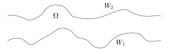
Figure 3.1. Two-dimensional infinitely long nozzle

Suppose that the nozzle has impermeable solid walls so that the flow satisfies the slip boundary condition:

$$u\cdot\nu=0\qquad\mbox{on}~{}\partial\Omega,$$ (3.3)

where $\nu$ is the unit outward normal to the nozzle wall.

It follows from $(\ref{CFE})_{1}$ and $(\ref{cdx-5})$ that

$$\int_{\Sigma}\,(\rho u)\cdot l\,{\rm d}s\equiv m$$ (3.4)

holds for some constant $m$, which is the mass flux, where $\Sigma$ is any curve transversal to the $x_{1}$–direction, and $l$ is the normal of $\Sigma$ in the positive $x_{1}$–axis direction.

We assume that the upstream entropy function is given, i.e.,

$$\frac{\rho}{p^{1/\gamma}}\longrightarrow S_{-}(x_{2})\qquad\mbox{as}~{}x_{1}\rightarrow-\infty,$$ (3.5)

and the upstream Bernoulli function is given, i.e.,

$$\frac{|u|^{2}}{2}+\frac{\gamma p}{(\gamma-1)\rho}\longrightarrow B_{-}(x_{2})\qquad\mbox{as}~{}x_{1}\rightarrow-\infty,$$ (3.6)

where $S_{-}(x_{2})$ and $B_{-}(x_{2})$ are the functions defined on $[0,1]$.

$\mathbf{Problem~{}1}(m,\gamma)$: Solve the full Euler system $(\ref{CFE})$ with the boundary condition $(\ref{cdx-5})$, the mass flux condition $(\ref{cdx-6})$, and the asymptotic conditions $(\ref{cdx-8})$–$(\ref{cdx-11})$.

Set

$$\underline{S}=\inf_{x_{2}\in[0,1]}S_{-}(x_{2}),\qquad\underline{B}=\inf_{x_{2}\in[0,1]}B_{-}(x_{2}).$$

For this problem, the following theorem has been established in Chen-Deng-Xiang [5].

Theorem 3.1.

Let the nozzle walls $\partial\Omega$ satisfy $(\ref{cdx-3})$–$(\ref{cdx-4})$, and let $\underline{S}>0$ and $\underline{B}>0$. Then there exists $\delta_{0}>0$ such that, if $\|(S_{-}-\underline{S},B_{-}-\underline{B})\|_{C^{1,1}([0,1])}\leq\delta$ for $0<\delta\leq\delta_{0}$, $(S_{-}B_{-})^{\prime}(0)\leq 0$, and $(S_{-}B_{-})^{\prime}(1)\geq 0$, there exists $\hat{m}\geq 2\delta_{0}^{\frac{1}{8}}$ such that, for any $m\in(\delta^{\frac{1}{4}},\hat{m})$, there is a global solution (i.e. a full Euler flow) $(\rho,u,p)\in C^{1,\alpha}(\overline{\Omega})$ of $\mathbf{Problem~{}1}(m,\gamma)$ such that the following hold:

(i) Subsonic state and horizontal direction of the velocity: The flow is uniformly subsonic with positive horizontal velocity in the whole nozzle, i.e.,

$$\sup_{\bar{\Omega}}(|u|^{2}-c^{2})<0,\quad u_{1}>0\qquad\mbox{in}~{}\bar{\Omega};$$ (3.7)

(ii) The flow satisfies the following asymptotic behavior in the far field: As $x_{1}\rightarrow-\infty$,

$$p\rightarrow p_{-}>0,\qquad u_{1}\rightarrow u_{-}(x_{2})>0,\qquad(u_{2},\rho)\rightarrow(0,\rho_{-}(x_{2};p_{-})),$$ (3.8)

$$\nabla p\rightarrow 0,\qquad\nabla u_{1}\rightarrow(0,u_{-}^{\prime}(x_{2})),\qquad\nabla u_{2}\rightarrow 0,\qquad\nabla\rho\rightarrow(0,\rho_{-}^{\prime}(x_{2};p_{-}))$$ (3.9)

uniformly for $x_{2}\in K_{1}\Subset(0,1)$, where $\rho_{-}(x_{2};p_{-})=p_{-}^{\frac{1}{\gamma}}S_{-}(x_{2})$, the constant $p_{-}$ and function $u_{-}(x_{2})$ can be determined by $m$, $S_{-}(x_{2})$, and $B_{-}(x_{2})$ uniquely.

Next, we take the incompressible limit of the full Euler flows.

Theorem 3.2 (Incompressible limit of two-dimensional full Euler flows).

Let $(\rho^{(\gamma)},u^{(\gamma)},p^{(\gamma)})(x)$ be the corresponding sequence of solutions to $\mathbf{Problem~{}1}(m^{(\gamma)},\gamma)$. Then, as $\gamma\rightarrow\infty$, the solution sequence possesses a subsequence (still denoted by) $(\rho^{(\gamma)},u^{(\gamma)},p^{(\gamma)})(x)$ that converges strongly a.e. in $\Omega$ to a vector function $(\bar{\rho},\bar{u},\bar{p})(x)$ which is a weak solution of $(\ref{ICIHE})$. Furthermore, the limit solution $(\bar{\rho},\bar{u},\bar{p})(x)$ also satisfies the boundary condition $(\ref{cdx-5})$ as the normal trace of the divergence-measure field $u$ on the boundary in the sense of Chen-Frid [6].

Proof. We divide the proof into four steps.

1. From $(\ref{CFE})$, we can obtain the following linear transport parts:

$$\begin{cases}\partial_{x_{1}}\big{(}(p^{(\gamma)})^{\frac{1}{\gamma}}u_{1}^{(\gamma)}\big{)}+\partial_{x_{2}}\big{(}(p^{(\gamma)})^{\frac{1}{\gamma}}u_{2}^{(\gamma)}\big{)}=0,\\[5.69054pt] \partial_{x_{1}}\big{(}(p^{(\gamma)})^{\frac{1}{\gamma}}B^{(\gamma)}u_{1}^{(\gamma)}\big{)}+\partial_{x_{2}}\big{(}(p^{(\gamma)})^{\frac{1}{\gamma}}B^{(\gamma)}u_{2}^{(\gamma)}\big{)}=0,\\[5.69054pt] \partial_{x_{1}}\big{(}(p^{(\gamma)})^{\frac{1}{\gamma}}S^{(\gamma)}u_{1}^{(\gamma)}\big{)}+\partial_{x_{2}}\big{(}(p^{(\gamma)})^{\frac{1}{\gamma}}S^{(\gamma)}u_{2}^{(\gamma)}\big{)}=0.\end{cases}$$ (3.10)

From $(\ref{3.2.1})_{1}$, we can introduce the potential function $\psi^{(\gamma)}$:

$$\begin{cases}\partial_{x_{1}}\psi^{(\gamma)}=-(p^{(\gamma)})^{\frac{1}{\gamma}}u_{2}^{(\gamma)},\\[5.69054pt] \partial_{x_{2}}\psi^{(\gamma)}=(p^{(\gamma)})^{\frac{1}{\gamma}}u_{1}^{(\gamma)}.\end{cases}$$ (3.11)

From the far-field behavior of the Euler flows, we can define

$$\psi^{(\gamma)}_{-}(x_{2}):=\lim\limits_{x_{1}\rightarrow-\infty}\psi^{(\gamma)}(x_{1},x_{2}).$$

Since both the upstream Bernoulli and entropy functions are given, $B^{(\gamma)}$ and $S^{(\gamma)}$ have the following expressions:

$$B^{(\gamma)}(x)=B_{-}((\psi^{(\gamma)}_{-})^{-1}(\psi^{(\gamma)}(x))),\qquad S^{(\gamma)}(x)=S_{-}((\psi^{(\gamma)}_{-})^{-1}(\psi^{(\gamma)}(x))),$$

where $(\psi^{(\gamma)}_{-})^{-1}\psi^{(\gamma)}(x)$ is a function from $\Omega$ to $[0,1]$, and

$$\begin{cases}B_{-}=\frac{u_{-}^{2}}{2}+\frac{\gamma}{\gamma-1}\frac{p_{-}}{\rho_{-}},\\[5.69054pt] S_{-}=\rho_{-}p_{-}^{-\frac{1}{\gamma}},\end{cases}$$

with uniformly upper and lower bounds with respect to $\gamma$.

Since the flow is subsonic so that the Mach number $M^{(\gamma)}\leq 1$, then we have

$$|u^{(\gamma)}|<\sqrt{\frac{2(\gamma-1)}{\gamma+1}\max B_{-}},$$ (3.12)

and

$$\left(\frac{2(\gamma-1)}{\gamma(\gamma+1)}\min(B_{-}S_{-})\right)^{\frac{\gamma}{\gamma-1}}<p^{(\gamma)}\leq\left(\frac{\gamma-1}{\gamma}\max(B_{-}S_{-})\right)^{\frac{\gamma}{\gamma-1}}.$$ (3.13)

Since $|u^{(\gamma)}|^{2}$ and $p^{(\gamma)}$ are uniformly bounded, we conclude that $|u^{(\gamma)}|^{2}$ and $p^{(\gamma)}$ are uniformly bounded in $L^{1}_{loc}(\Omega)$. Thus, conditions (A.1)–(A.2) are satisfied. It is observed that, even though the lower bound of pressure $p^{(\gamma)}$ may tend to zero as $\gamma\to\infty$ with polynomial rate, so that (F.1) holds for any bounded domain.

2. For fixed $x_{1}$, $(\psi^{\gamma}_{-})^{-1}(\psi^{\gamma}(\cdot))$ can be regarded as a backward characteristic map with

$$\frac{\partial((\psi^{(\gamma)}_{-})^{-1}(\psi^{(\gamma)}))}{\partial x_{2}}=\frac{(p^{(\gamma)})^{\frac{1}{\gamma}}u^{(\gamma)}_{1}}{p_{-}^{\frac{1}{\gamma}}u_{-}}>0.$$

The uniform boundedness and positivity of $p_{-}^{\frac{1}{\gamma}}u_{-}$ and $(p^{(\gamma)})^{\frac{1}{\gamma}}u^{(\gamma)}_{1}$ implies that the map is not degenerate. Then we have

$$\begin{cases}\partial_{x_{1}}S^{(\gamma)}(x)=-S_{-}^{\prime}((\psi^{(\gamma)}_{-})^{-1}(\psi^{(\gamma)}(x)))\frac{(p^{(\gamma)})^{\frac{1}{\gamma}}u^{(\gamma)}_{2}}{p_{-}^{\frac{1}{\gamma}}u_{-}},\\[5.69054pt] \partial_{x_{2}}S^{(\gamma)}(x)=S_{-}^{\prime}((\psi^{(\gamma)}_{-})^{-1}(\psi^{(\gamma)}(x)))\frac{(p^{(\gamma)})^{\frac{1}{\gamma}}u^{(\gamma)}_{1}}{p_{-}^{\frac{1}{\gamma}}u_{-}}.\end{cases}$$ (3.14)

Thus, $S^{(\gamma)}$ is uniformly bounded in $BV$, which implies its strong convergence. Then condition (F.2) follows.

3. Similar to [7], the vorticity sequence $\omega^{(\gamma)}:=\partial_{x_{1}}u_{2}^{(\gamma)}-\partial_{x_{2}}u_{1}^{(\gamma)}$ can be written as

$$\begin{cases}\partial_{x_{1}}B^{(\gamma)}=u_{2}^{(\gamma)}\omega^{(\gamma)}-\frac{\gamma}{\gamma-1}(\rho^{(\gamma)})^{-2}(p^{(\gamma)})^{\frac{\gamma+1}{\gamma}}\partial_{x_{1}}S^{(\gamma)},\\[5.69054pt] \partial_{x_{2}}B^{(\gamma)}=-u_{1}^{(\gamma)}\omega^{(\gamma)}-\frac{\gamma}{\gamma-1}(\rho^{(\gamma)})^{-2}(p^{(\gamma)})^{\frac{\gamma+1}{\gamma}}\partial_{x_{2}}S^{(\gamma)}.\end{cases}$$ (3.15)

By direct calculation, we have

$$\omega^{(\gamma)} = \frac{1}{|u^{(\gamma)}|^{2}}\Big{(}u_{2}^{(\gamma)}\big{(}\partial_{x_{1}}B^{(\gamma)}+\frac{\gamma}{\gamma-1}(\rho^{(\gamma)})^{-2}(p^{(\gamma)})^{\frac{\gamma+1}{\gamma}}\partial_{x_{1}}S^{(\gamma)}\big{)}$$ (3.16)

$$\qquad\qquad-u_{1}^{(\gamma)}\big{(}\partial_{x_{2}}B^{(\gamma)}+\frac{\gamma}{\gamma-1}(\rho^{(\gamma)})^{-2}(p^{(\gamma)})^{\frac{\gamma+1}{\gamma}}\partial_{x_{2}}S^{(\gamma)}\big{)}\Big{)}$$

$$= -\frac{1}{p_{-}^{\frac{1}{\gamma}}u_{-}}\Big{(}(p^{(\gamma)})^{\frac{1}{\gamma}}B_{-}^{\prime}+\frac{\gamma}{\gamma-1}(p^{(\gamma)})^{\frac{\gamma+2}{\gamma}}(\rho^{(\gamma)})^{-2}S_{-}^{\prime}\Big{)},$$

which implies that $\omega^{\varepsilon}$ as a measure sequence is uniformly bounded so that it is compact in $H^{-1}_{loc}$. Therefore, the flows satisfy condition (A.3).

Then Proposition 2.4 immediately implies that the solution sequence has a subsequence (still denoted by) $(\rho^{(\gamma)},u^{(\gamma)},p^{(\gamma)})(x)$ that converges a.e. in $\Omega$ to a vector function $(\bar{\rho},\bar{u},\bar{p})(x)$ as $\gamma\to\infty$.

4. Since $\bar{u}$ is uniformly bounded, the normal trace $\bar{u}\cdot\nu$ on $\partial\Omega$ exists and is in $L^{\infty}(\partial\Omega)$ in the sense of Chen-Frid [6]. On the other hand, for any $\phi\in C^{\infty}(\mathbb{R}^{2})$, we have

$$\langle(\bar{u}\cdot\nu)|_{\partial\Omega},\phi\rangle=\int_{\Omega}\bar{u}(x)\cdot\nabla\phi(x)\,{\rm d}x+\int_{\Omega}\phi\mbox{div}\,\bar{u}\,{\rm d}x.$$ (3.17)

Since $\int_{\Omega}\phi\,\mbox{div}\,\bar{u}\,{\rm d}x=0$, and

$$\int_{\Omega}\bar{u}(x)\cdot\nabla\phi(x)\,{\rm d}x=\lim\limits_{\gamma\rightarrow\infty}\int_{\Omega}((p^{(\gamma)})^{\frac{1}{\gamma}}u^{(\gamma)})(x)\cdot\nabla\phi(x)\,{\rm d}x=0,$$ (3.18)

then we have

$$\langle(\bar{u}\cdot\nu)|_{\partial\Omega},\phi\rangle=0,$$ (3.19)

for any $\phi\in C^{\infty}(\mathbb{R}^{2})$. By approximation, we conclude that the normal trace $(\bar{u}\cdot\nu)|_{\partial\Omega}=0$ in $L^{\infty}(\partial\Omega)$. This completes the proof.

Remark 3.1.

In the two-dimensional homentropic case, the subsonic results in [2, 28] can also be extended to the incompressible limit by using Proposition 2.3.

4. Incompressible Limit for the Three-Dimensional Homentropic Euler Flows in an Infinitely Long Axisymmetric Nozzle

We consider Euler flows through an infinitely long axisymmetric nozzle in $\mathbb{R}^{3}$ given by

$$\Omega=\{(x_{1},x_{2},x_{3})\in\mathbb{R}^{3}\,:\,0\leq\sqrt{x_{2}^{2}+x_{3}^{2}}<f(x_{1}),~{}-\infty<x_{1}<\infty\},$$

where $f(x_{1})$ satisfies

$$f(x_{1})\rightarrow 1\qquad\mbox{as}~{}x_{1}\rightarrow-\infty,$$

$$f(x_{1})\rightarrow r_{0}\qquad\mbox{as}~{}x_{1}\rightarrow\infty,$$

$$\|f\|_{C^{2,\alpha}(\mathbb{R})}\leq C\qquad\mbox{for}~{}\mbox{some}~{}\alpha>0~{}\mbox{and}~{}C>0,$$ (4.1)

$$\inf_{x_{1}\in\mathbb{R}}f(x_{1})=b>0.$$ (4.2)

See Fig. 4.1.

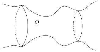
Figure 4.1. Infinitely long axisymmetric nozzle

The boundary condition is set as follows: Since the nozzle wall is solid, the flow satisfies the slip boundary condition:

$$u\cdot\nu=0\qquad\mbox{on}~{}\partial\Omega,$$ (4.3)

where $\nu$ is the unit outward normal to the nozzle wall. The continuity equation in $(\ref{CFE})_{1}$ and the boundary condition $(\ref{dL-3})$ imply that the mass flux

$$\int_{\Sigma}\,(\rho u)\cdot l\,{\rm d}s\equiv m_{0}$$ (4.4)

remains for some positive constant $m_{0}$, where $\Sigma$ is any surface transversal to the $x_{1}$–axis direction, and $l$ is the normal of $\Sigma$ in the positive $x_{1}$–axis direction.

In Du-Duan [13], axisymmetric flows without swirl are considered for the fluid density $\rho=\rho(x_{1},r)$ and the velocity

$$u=(u_{1},u_{2},u_{3})=(U(x_{1},r),V(x_{1},r)\frac{x_{2}}{r},V(x_{1},r)\frac{x_{3}}{r})$$

in the cylindrical coordinates, where $u_{1}$, $u_{2}$, and $u_{3}$ are the axial velocity, radial velocity, and swirl velocity, respectively, and $r=\sqrt{x_{2}^{2}+x_{3}^{2}}$. Then, instead of $(\ref{CISE})$, we have

$$\left\{\begin{split}&\partial_{x_{1}}(r\rho U)+\partial_{r}(r\rho V)=0,\\[2.84526pt] &\partial_{x_{1}}(r\rho U^{2})+\partial_{r}(r\rho UV)_{r}+r\partial_{x_{1}}p=0,\\[2.84526pt] &\partial_{x_{1}}(r\rho UV)+\partial_{r}(r\rho V^{2})_{r}+r\partial_{r}p=0.\end{split}\right.$$ (4.5)

Rewrite the axisymmetric nozzle as

$$\Omega=\{(x_{1},r)\,:\,0\leq r<f(x_{1}),~{}-\infty<x_{1}<\infty\}$$

with the boundary of the nozzle:

$$\partial\Omega=\{(x_{1},r)\,:\,r=f(x),~{}-\infty<x_{1}<\infty\}.$$

The boundary condition $(\ref{dL-3})$ becomes

$$(U,V,0)\cdot\tilde{\nu}=0\qquad\mbox{on}~{}\partial\Omega,$$ (4.6)

where $\tilde{\nu}$ is the unit outer normal of the nozzle wall in the cylindrical coordinates. The mass flux condition $(\ref{dd-4})$ can be rewritten in the cylindrical coordinates as

$$\int_{\Sigma}(r\rho U,r\rho V,0)\cdot\tilde{l}\,{\rm d}s\equiv m:=\frac{m_{0}}{2\pi},$$ (4.7)

where $\Sigma$ is any curve transversal to the $x_{1}$-axis direction, and $\tilde{l}$ is the unit normal of $\Sigma$.

Notice that the quantity

$$B=\frac{\gamma}{\gamma-1}\rho^{\gamma-1}+\frac{U^{2}+V^{2}}{2}$$

is constant along each streamline. For the homentropic Euler flows in the axisymmetric nozzle, we assume that the upstream Bernoulli is given, that is,

$$\frac{\gamma}{\gamma-1}\rho^{\gamma-1}+\frac{U^{2}+V^{2}}{2}\longrightarrow B_{-}(r)\qquad\mbox{as}~{}x_{1}\rightarrow-\infty,$$ (4.8)

where $B_{-}(r)$ is a function defined on $[0,1]$.

Set

$$\underline{B}=\inf\limits_{r\in[0,1]}B_{-}(r),\quad\sigma=||B^{\prime}_{-}||_{C^{0,1}([0,1])},$$ (4.9)

We denote the above problem as $\mathbf{Problem~{}2}(m,\gamma)$. It is shown in [13] that

Theorem 4.1.

Suppose that the nozzle satisfies $(\ref{dd-2})$. Let the upstream Bernoulli function $B(r)$ satisfy $\underline{B}>0$, $B^{\prime}(r)\in C^{1,1}([0,1])$, $B^{\prime}(0)=0$, and $B^{\prime}(r)\geq 0$ on $r\in[0,1]$. Then we have

1. There exists $\delta_{0}>0$ such that, if $\sigma\leq\delta_{0}$, then there is $\hat{m}\leq 2\delta_{0}^{\frac{1}{8}}$. For any $m\in(\delta_{0}^{\frac{1}{4}},\hat{m})$, there exists a global $C^{1}$–solution (i.e. a homentropic Euler flow) $(\rho,U,V)\in C^{1}(\overline{\Omega})$ through the nozzle with mass flux condition $(\ref{dd-9})$ and the upstream asymptotic condition $(\ref{dd-13})$. Moreover, the flow is uniformly subsonic, and the axial velocity is always positive, i.e.,

   $$\sup_{\bar{\Omega}}(U^{2}+V^{2}-c^{2})<0\quad\mbox{and}\quad U>0\qquad\mbox{in}~{}\overline{\Omega}.$$ (4.10)

2. The subsonic flow satisfies the following properties: As $x_{1}\rightarrow-\infty$,

   $$\rho\rightarrow\rho_{-}>0,\quad\nabla\rho\rightarrow 0,\quad p\rightarrow\rho_{-}^{\gamma},\quad(U,V)\rightarrow(U_{-}(r),0),\quad\nabla U\rightarrow(0,U_{-}^{\prime}(r)),$$ (4.11)

   uniformly for $r\in K_{1}\Subset(0,1)$, where $\rho_{-}$ is a positive constant, and $\rho_{-}$ and $U_{-}(r)$ can be determined by $m$ and $B(r)$ uniquely.

As above, we have the following incompressible limit theorem for this case.

Theorem 4.2 (Incompressible limit of three-dimensional Euler flows through an axisymmetric nozzle).

Let $u^{(\gamma)}=(u^{(\gamma)}_{1},u^{(\gamma)}_{2},u^{(\gamma)}_{3})$, and $p^{(\gamma)}=(\rho^{(\gamma)})^{\gamma}$ be the corresponding solutions to $\mathbf{Problem~{}2}~{}(m^{(\gamma)},\gamma)$. Then, as $\gamma\rightarrow\infty$, the solution sequence possesses a subsequence (still denoted by) $(u^{(\gamma)},p^{(\gamma)})$ that converges strongly a.e. in $\Omega$ to a vector function $(\bar{u},\bar{p})$ with $\bar{u}=(\bar{u}_{1},\bar{u}_{2},\bar{u}_{3})$ which is a weak solution of $(\ref{ICHE})$. Furthermore, the limit solution $(\bar{u},\bar{p})$ also satisfies the boundary conditions $(\ref{dL-3})$ as the normal trace of the divergence-measure field $(\bar{u}_{1},\bar{u}_{2},\bar{u}_{3})$ on the boundary in the sense of Chen-Frid [6].

Proof. For the approximate solutions, $B^{(\gamma)}$ satisfy

$$\partial_{x_{1}}(rU^{(\gamma)}(p^{(\gamma)})^{\frac{1}{\gamma}}B^{(\gamma)})+\partial_{r}(rV^{(\gamma)}(p^{(\gamma)})^{\frac{1}{\gamma}}B^{(\gamma)})=0.$$ (4.12)

Based on the equation:

$$\partial_{x_{1}}(rU^{(\gamma)}(p^{(\gamma)})^{\frac{1}{\gamma}})+\partial_{r}(rV^{(\gamma)}(p^{(\gamma)})^{\frac{1}{\gamma}})=0,$$

we introduce $\psi^{(\gamma)}$ as

$$\begin{cases}\partial_{x_{1}}\psi^{(\gamma)}=-rV^{(\gamma)}(p^{(\gamma)})^{\frac{1}{\gamma}},\\[5.69054pt] \partial_{r}\psi^{(\gamma)}=rU^{(\gamma)}(p^{(\gamma)})^{\frac{1}{\gamma}}.\end{cases}$$ (4.13)

From the far-field behavior of the Euler flows, we define

$$\psi^{(\gamma)}_{-}(r):=\lim\limits_{x_{1}\rightarrow-\infty}\psi^{(\gamma)}(x_{1},r).$$

Similar to the argument in Theorem 3.2, $(\psi^{(\gamma)}_{-})^{-1}(\psi^{(\gamma)})$ are nondegenerate maps. A direct calculation yields

$$B^{(\gamma)}(x_{1},x_{2},x_{3})=B_{-}((\psi^{(\gamma)}_{-})^{-1}(\psi^{(\gamma)}(x_{1},\sqrt{x_{2}^{2}+x_{3}^{2}}))),$$

with

$$B^{(\gamma)}_{-}=\frac{U_{-}^{2}}{2}+\frac{\gamma}{\gamma-1}\rho_{-}^{\gamma-1},$$ (4.14)

Similar to the previous case, the flow is subsonic so that the Mach number $M^{(\gamma)}\leq 1$,

$$|(U^{(\gamma)},V^{(\gamma)})|<\sqrt{2\max B_{-}},$$ (4.15)

and

$$\left(\frac{2(\gamma-1)}{\gamma(\gamma+1)}\min B_{-}\right)^{\frac{\gamma}{\gamma-1}}<p^{(\gamma)}\leq\left(\frac{\gamma-1}{\gamma}\max B_{-}\right)^{\frac{\gamma}{\gamma-1}}.$$ (4.16)

From (1.4), we have

$$\frac{2}{\gamma(\gamma+1)}\min B_{-}<E^{(\gamma)}\leq\frac{(\gamma-1)\gamma+2}{2\gamma}\max B_{-}.$$ (4.17)

Therefore, conditions (A.1)–(A.2) and (H) are satisfied for any bounded domain.

On the other hand, the vorticity $\omega^{(\gamma)}$ has the following expressions:

$$\begin{cases}\omega_{1,2}^{(\gamma)}=\partial_{x_{1}}u_{2}^{(\gamma)}-\partial_{x_{2}}u_{1}^{(\gamma)}=\frac{x_{2}}{r}(\partial_{x_{1}}V^{(\gamma)}-\partial_{r}U^{(\gamma)}),\\[5.69054pt] \omega_{2,3}^{(\gamma)}=\partial_{x_{2}}u_{3}^{(\gamma)}-\partial_{x_{3}}u_{2}^{(\gamma)}=0,\\[5.69054pt] \omega_{3,1}^{(\gamma)}=\partial_{x_{3}}u_{1}^{(\gamma)}-\partial_{x_{1}}u_{3}^{(\gamma)}=-\frac{x_{3}}{r}(\partial_{x_{1}}V^{(\gamma)}-\partial_{r}U^{(\gamma)}).\end{cases}$$ (4.18)

A direct calculation yields

$$\partial_{x_{1}}V^{(\gamma)}-\partial_{r}U^{(\gamma)}=-\frac{r}{p_{-}^{\frac{1}{\gamma}}U_{-}}(p^{(\gamma)})^{\frac{1}{\gamma}}B_{-}^{\prime},$$ (4.19)

which implies that $\omega^{(\gamma)}$ is uniformly bounded in the bounded measure space and (A.3) is satisfied.

Then the sequence $(u^{(\gamma)},p^{(\gamma)})(x)$ satisfies conditions (A.1)–(A.3) and (H). Moreover, $(\ref{CISE})$ holds for $(u^{(\gamma)},p^{(\gamma)})(x)$.

Similar to Theorem 3.2, we conclude that there exists a subsequence (still denoted by) $(u^{(\gamma)},p^{(\gamma)})$ that converges to a vector function $(\bar{u},\bar{p})$ a.e. in $\Omega$ satisfying (1.11) in the distributional sense.

Since $\bar{u}$ is uniformly bounded, the normal trace $\bar{u}\cdot\nu$ on $\partial\Omega$ exists and is in $L^{\infty}(\partial\Omega)$ in the sense of Chen-Frid [6]. On the other hand, for any $\phi\in C^{\infty}(\mathbb{R}^{2})$, we have

$$\langle(\bar{u}\cdot\nu)|_{\partial\Omega},\phi\rangle=\int_{\Omega}\bar{u}(x)\cdot\nabla\phi(x)\,{\rm d}x+\int_{\Omega}\phi\,\mbox{div}\,\bar{u}\,{\rm d}x.$$ (4.20)

Since $\int_{\Omega}\phi\,\mbox{div}\,\bar{u}\,{\rm d}x=0$, and

$$\int_{\Omega}\bar{u}(x)\cdot\nabla\phi(x)\,{\rm d}x=0,$$ (4.21)

then we have

$$\langle(\bar{u}\cdot\nu)|_{\partial\Omega},\phi\rangle=0,$$ (4.22)

for any $\phi\in C^{\infty}(\mathbb{R}^{2})$. By approximation, we conclude that the normal trace $(\bar{u}\cdot\nu)|_{\partial\Omega}=0$ in $L^{\infty}(\partial\Omega)$. This completes the proof.

Remark 4.1.

For the full Euler flow case, the subsonic results of [14] can be also extended to the incompressible limit by Proposition 2.4.

Acknowledgments: The research of Gui-Qiang G. Chen was supported in part by the UK EPSRC Science and Innovation Award to the Oxford Centre for Nonlinear PDE (EP/E035027/1), the UK EPSRC Award to the EPSRC Centre for Doctoral Training in PDEs (EP/L015811/1), and the Royal Society–Wolfson Research Merit Award (UK). The research of Feimin Huang was supported in part by NSFC Grant No. 10825102 for distinguished youth scholars, and the National Basic Research Program of China (973 Program) under Grant No. 2011CB808002. The research of Tianyi Wang was supported in part by the China Scholarship Council No. 201204910256 as an exchange graduate student at the University of Oxford, the UK EPSRC Science and Innovation Award to the Oxford Centre for Nonlinear PDE (EP/E035027/1), and the NSFC Grant No. 11371064; He would like to thank Professor Zhouping Xin for the helpful discussions. Wei Xiang was supported in part by the UK EPSRC Science and Innovation Award to the Oxford Centre for Nonlinear PDE (EP/E035027/1), the CityU Start-Up Grant for New Faculty 7200429(MA), and the General Research Fund of Hong Kong under GRF/ECS Grant 9048045 (CityU 21305215).

References

• [1] J. Ball, A version of the fundamental theorem of Young measures, In: PDEs and Continuum Models of Phase Transitions, pp. 207–215. Lecture Notes in Physics, 344, Springer-Verlag, 1989.
• [2] C. Chen and C.-J. Xie, Existence of steady subsonic Euler flows through infinitely long periodic nozzles. J. Diff. Eqs. 252 (2012), 4315–4331.
• [3] G.-Q. Chen, C. Christoforou, and Y. Zhang, Continuous dependence of entropy solutions to the Euler equations on the adiabatic exponent and Mach number. Arch. Rational Mech. Anal. 189(1) (2008), 97–130.
• [4] G.-Q. Chen, C. M. Dafermos, M. Slemrod, and D.-H. Wang, On two-dimensional sonic-subsonic flow. Commun. Math. Phys. 271 (2007), 635–647.
• [5] G.-Q. Chen, X. Deng, and W. Xiang, Global steady subsonic flows through infinitely long nozzles for the full Euler equations. SIAM J. Math. Anal. 44 (2012), 2888–2919.
• [6] G.-Q. Chen and H. Frid, Divergence-measure fields and hyperbolic conservation laws. Arch. Rational Mech. Anal. 147 (1999), 89–118.
• [7] G.-Q. Chen, F.-M. Huang, and T.-Y. Wang, Subsonic-sonic limit of approximate solutions to multidimensional steady Euler equations. Arch. Rational Mech. Anal. bf 219 (2016), 719–740.
• [8] R. Courant and K.O. Friedrichs, Supersonic Flow and Shock Waves, Interscience Publishers Inc.: New York, 1948.
• [9] C. M. Dafermos, Hyperbolic Conservation Laws in Continuum Physics. Springer-Verlag: Berlin, 2010.
• [10] B. Desjardins and E. Grenier, Low Mach number limit of viscous compressible flows in the whole space. R. Soc. Lond. Proc. Ser. A: Math. Phys. Eng. Sci. 455 (1999), 2271–2279.
• [11] B. Desjardins, E. Grenier, P.-L. Lions, and N. Masmoudi, Incompressible limit for solutions of the isentropic Navier-Stokes equations with Dirichlet boundary conditions. J. Math. Pures Appl. 78 (1999), 461–471.
• [12] R. DiPerna, Compensated compactness and general systems of conservation laws. Trans. Amer. Math. Soc. 292 (1985), 383–420.
• [13] L.-L. Du and B. Duan, Global subsonic Euler flows in an infinitely long axisymmetric nozzle. J. Diff. Eqs. 250 (2011), 813–847.
• [14] B. Duan and Z. Luo, Three-dimensional full Euler flows in axisymmetric nozzles. J. Diff. Eqs. 254 (2013), 2705–2731.
• [15] F.-M. Huang, T.-Y. Wang, and Y. Wang, On multidimensional sonic-subsonic flow. Acta Math. Sci. Ser. B, 31 (2011), 2131–2140.
• [16] S. Klainerman and A. Majda, Singular perturbations of quasilinear hyperbolic systems with large parameters and the incompressible limit of compressible fluids. Comm. Pure Appl. Math. 34 (1981) 481–524.
• [17] S. Klainerman and A. Majda, Compressible and incompressible fluids. Comm. Pure Appl. Math. 35 (1982), 629–653.
• [18] S. Labbé and E. Maitre, A free boundary model for Korteweg fluids as a limit of barotropic compressible Navier-Stokes equations. Meth. Appl. Anal. 20 (2013), 165–178.
• [19] P.-L. Lions, Mathematical Topics in Fluid Dynamics. Vol. 1. Incompressible Models, Oxford Univ. Press: London, 1996.
• [20] P.-L. Lions and N. Masmoudi, Incompressible limit for a viscous compressible fluid. J. Math. Pures Appl. 77 (1998) 585–627.
• [21] P.-L. Lions and N. Masmoudi, On a free boundary barotropic model. Ann. Inst. H. Poincar$\acute{e}$ Anal. Non Lin$\acute{e}$aire, 16 (1999) 373–410.
• [22] N. Masmoudi, Asymptotic problems and compressible-incompressible limit. In: Advances in mathematical fluid mechanics, pp. 119–158, Springer-Verlag, 2000.
• [23] N. Masmoudi, Examples of singular limits in hydrodynamics. Handbook of Differential Equations: Evolutionary Equations, 3, pp. 195–275, 2007.
• [24] F. Murat, Compacite par compensation. Ann. Suola Norm. Pisa (4), 5 (1978), 489–507.
• [25] D. Serre, Systems of Conservation Laws, Vols. 12, Cambridge University Press: Cambridge, 1999, 2000.
• [26] L. Tartar, Compensated compactness and applications to partial differential equations. In: Nonlinear Analysis and Mechanics: Herriot-Watt Symposium, Vol. 4, Ed. R. J. Knops, Pitman Press, 1979.
• [27] S. Ukai, The incompressible limit and the initial layer of the compressible Euler equation. J. Math. Kyoto Univ. 26 (1986), 323–331.
• [28] C. Xie and Z. Xin, Existence of global steady subsonic Euler flows through infinitely long nozzles. SIAM J. Math. Anal. 42 (2010), 751–784.