Hamiltonian Properties of DCell Networks

Abstract.

DCell has been proposed for data centers as a server centric interconnection network structure. DCell can support millions of servers with high network capacity by only using commodity switches. With one exception, we prove that a $k$ level DCell built with $n$ port switches is Hamiltonian-connected for $k\geq 0$ and $n\geq 2$. Our proof extends to all generalized DCell connection rules for $n\geq 3$. Then, we propose an $O(t_{k})$ algorithm for finding a Hamiltonian path in $DCell_{k}$, where $t_{k}$ is the number of servers in $DCell_{k}$. What’s more, we prove that $DCell_{k}$ is $(n+k-4)$-fault Hamiltonian-connected and $(n+k-3)$-fault Hamiltonian. In addition, we show that a partial DCell is Hamiltonian connected if it conforms to a few practical restrictions.

1. Introduction

Data centers are critical to the business of companies such as Amazon, Google, Facebook, and Microsoft. These and other corporations operate data centers with hundreds of thousands of servers. Their operations are important to offer both many on-line applications such as web search, on-line gaming, email, cloud storage, and infrastructure services such as GFS [7], Map-reduce [3], and Dryad [10]. The growth in demand for such services has lately exceeded the growth in performance afforded by existing data center technology and topology. In particular, we are faced by the challenge of interconnecting a large number of servers in one data center, at a low cost, and without compromising performance. Toward this end, Al-Fares et al. [1] introduced the idea of replacing high-end networking hardware with commodity switches in a data center network called Fat-tree. Concurrently, Guo et al. proposed a server-centric data center network called DCell [9], wherein the commodity switches have no intelligence at all, and all of the routing intelligence is restricted to the servers.

DCell is particularly apt to handle a very large number of servers, even on the order of millions. It scales double exponentially in the number of ports in each server, it has high network capacity, large bisection width, small diameter, and high fault-tolerance. DCell only requires mini-switches and can support a scalable routing algorithm.

DCell is part of a class of data center network designs that evolved from parallel computing interconnects (see [15]), where Hamiltonian cycles and paths are commonly used for making low congestion and deadlock-free message broadcasts (e.g [16, 19]). Although the applications and traffic of high performance parallel computing and data center networks differ from each other, broadcasts are likely to be used in a data center in order to update information about the network, perform distributed computations, etc. For example, broadcasting is implemented both in DCell and BCube [8]. It is natural to consider Hamiltonian broadcast schemes in such server-centric data centres, especially when slower broadcasts are acceptable and bandwidth conservation is critical.

It is well known that there is no nontrivial necessary and sufficient condition for a graph to be Hamiltonian, and that finding a Hamiltonian cycle or path is NP-Complete [6, 11]. Therefore, a large amount of research on Hamiltonicity focuses on different special networks. Fan showed that the $n$-dimensional Möbius cube $M_{n}$ is Hamiltonian-connected when $n\geq 3$ [5]. Park et al. showed that every restricted hypercube-like interconnection networks of degree $m$$(m\geq 3)$ is $(m-3)$-fault Hamiltonian-connected and $(m-2)$-fault Hamiltonian [17]. Let $G$ be an $n$-dimensional twisted hypercube-like networks with $n\geq 7$ and let $F$ be a subset of $V(G)\cup E(G)$ with $|F|\leq 2n-9$. Yang et al. proved that $G\backslash F$ contains a Hamiltonian cycle if $\delta(G\backslash F)\geq 2$ [21]. Wang treated the problem of embedding Hamiltonian cycles into a crossed cube with failed links and found a Hamiltonian cycle in a crossed cubes $CQ_{n}$ tolerating up to $n-2$ failed links [18]. Xu et al. provided a systematic method to construct a Hamiltonian path in Honeycomb meshes [20].

A flood-like broadcast scheme for DCell, called DCellBroadcast, is used in [9] instead of a tree-like multicast, because it is fault tolerant. DCellBroadcast creates congestion because the broadcast message is replicated many times, and for bandwidth-critical applications it is worth revisiting the broadcast problem. In doing so, we explore the avenue of Hamiltonian cycle or path based multicast routing, inspired by those in parallel computing ([16, 19]).

So far, there is no work reported about the Hamiltonian properties of DCell. The major contributions of this paper are as follows:

1. We prove that a $k$ level DCell built with $n$ port switches is Hamiltonian-connected for $k\geq 0$ and $n\geq 2$, except for $(k,n)=(1,2)$,

2. we prove that a $k$ level Generalized DCell [13] built with $n$ port switches is Hamiltonian-connected for $k\geq 0$ and $n\geq 3$,

3. we propose an $O(t_{k})$ algorithm for finding a Hamiltonian path in $DCell_{k}$, where $t_{k}$ is the number of servers in $DCell_{k}$,

4. we prove that a $k$ level $DCell$ with up to $(n+k-4)$-faulty components is Hamiltonian-connected and with up to $(n+k-3)$-faulty components is Hamiltonian, and,

5. we prove that a partial DCell is Hamiltonian-connected if it conforms to a few practical restrictions.

This work is organized as follows. Section 2 provides the preliminary knowledge. Our main result, that DCell is Hamiltonian-connected, is given in Section 3. Section 4 discusses fault-tolerant Hamiltonian properties of DCell. Hamiltonian properties in partial DCells are given in Section 5. We provide some discussions in Section 6. We make a conclusion in Section 7.

2. Preliminaries

Let a data center network be represented by a simple graph $G=\left(V\left(G\right),E\left(G\right)\right)$, where $V\left(G\right)$ represents the vertex set and $E\left(G\right)$ represents the edge set, and each vertex represents a server and each edge represents a link between servers (switches can be regarded as transparent network devices [9]). The edge between vertices $u$ and $v$ is denoted by $(u,v)$. In this paper all graphs are simple and undirected.

A $(u_{0},u_{n})$-path of length $n$ in a graph is a sequence of vertices, $P:(u_{0},u_{1},\dots,u_{j},\dots u_{n-1},u_{n})$, in which no vertices are repeated and $u_{j},u_{j+1}$ are adjacent for any integer $0\leq j<n$. We use $V(P)$ and $E(P)$ to denote the vertices and edges of $P$, respectively. If $u$ and $v$ are vertices on a path $Q$, we write $P(Q,u,v)$ to denote the sub-path of $Q$ from $u$ to $v$. If $P_{2}$ contains only the edge $(v,w)$, we simply write $P_{1}+(v,w)$, and furthermore, we allow the subtractive analog, so that $(P_{1}+(v,w))-(v,w)=P_{1}$.

A $(u,v)$-path in a graph $G$ containing every vertex of $G$ is called a Hamiltonian path, and it is denoted $HP(u,v,G)$. If $(v,u)\in E(G)$, then $HP(u,v,G)+(u,v)$ is a Hamiltonian cycle $C$. Thus, we say $C-(u,v)$ is a Hamiltonian path $HP(u,v,G)$. A Hamiltonian graph is a graph containing a Hamiltonian cycle. If there exists a Hamiltonian path between any two distinct vertices of $G$, then $G$ is Hamiltonian-connected. It is easy to see that if $G$ is a Hamiltonian-connected graph with $|V(G)|\geq 3$, then $G$ must be a Hamiltonian graph.

For undefined graph theoretic terms see [4].

DCell uses a recursively defined structure to interconnect servers. Each server connects to different levels of DCell through multiple links. We build high-level DCell recursively to form many low-level ones.

According to the definition of $DCell_{k}$ [9], we provide the recursive definition as Definition 1.

Definition 1 (DCell, [9]).

Let $D_{k}$ denote a level $k$ DCell, for each $k\geq 0$ and some global constant $n$. Let $D_{0}=K_{n}$, and let $t_{k}$ denote the number of vertices in $D_{k}$ (thus $t_{0}=n$).

For $k>0$, the graph $D_{k}$ is built from $t_{k-1}+1$ disjoint copies of $D_{k-1}$, where $D^{i}_{k-1}$ denotes the $i$th copy. Each pair of DCells, $(D^{a}_{k-1},D^{b}_{k-1})$, is connected by a level $k$ edge, $(u,v)$, according to the rule described in Connection rule, below. We say that $v$ is the (unique) level $k$ neighbor of $u$.

A vertex $x$ (of $D_{k}$) in $D_{k-1}^{i}$ is labeled $(i,\alpha_{k-1},\ldots,\alpha_{0})$ where $k>0$, and $\alpha_{0}\in\{1,2,\ldots,n\}$.

The suffix, $(\alpha_{j},\alpha_{j-1},\ldots,\alpha_{0})$, of the label $\alpha$, has the unique uid_j, given by $uid_{j}(\alpha)=\alpha_{0}+\sum_{l=1}^{j}(\alpha_{l}t_{l-1})$. In $D_{k}$, each vertex is uniquely identified by its full label, or alternatively, by a $uid_{j}$ and the corresponding prefix of the label.

Connection rule::

For each pair of level $k-1$ DCells, $(D^{a}_{k-1},D^{b}_{k-1})$, with $a<b$, vertex uid_k-1 $b-1$ of $D^{a}_{k-1}$ is connected to vertex uid_k-1 $a$ of $D^{b}_{k-1}$.

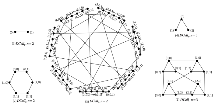
Figure 1. Small DCells and some special cases with regards Hamiltonian connectivity.

Figure 1 depicts several DCells with small parameters $n$ and $k$.

Definition 1 generalizes by replacing the connection rule with a different one that satisfies the requirement that each vertex be incident with exactly one level $k$ edge (see [9]). We have indicated where our results apply to Generalized DCell, but $D_{k}$ and $DCell_{k}$ refers to the connection rule in Definition 1 unless otherwise stated.

3. Hamiltonian Connectivity of DCell

In this section we prove by induction on $k$, that $\text{DCell}_{k}$ is Hamiltonian Connected in all but a few inconsequential cases. The base cases are given as Lemmas 1-4, and the main result is Theorem 1. We indicate wherever the results also hold for generalized DCell, but $D_{k}$ and $DCell_{k}$ continue to refer to the graph in Definition 1. Furthermore, we propose an $O(t_{k})$ algorithm for finding a Hamiltonian path in $DCell_{k}$, where $t_{k}$ is the number of servers in $DCell_{k}$.

Lemma 1.

For any integer $n$ with $n\geq 2$, (Generalized) $DCell_{0}$ is Hamiltonian-connected.

Proof.

The lemma holds, since $DCell_{0}$ is a complete graph [4]. ∎

Lemma 2.

$DCell_{1}$ is a Hamiltonian graph with $n=2$. However, $DCell_{1}$ is not Hamiltonian-connected with $n=2$. This also holds for Generalized DCell.

Proof.

$DCell_{1}$ is a cycle on 6 vertices. Therefore, for $n=2$, $DCell_{1}$ is a Hamiltonian graph, and $DCell_{1}$ is not Hamiltonian-connected [4]. ∎

Lemma 3.

$DCell_{2}$ is Hamiltonian-connected with $n=2$. This does not hold for all Generalized DCell, specifically, not for $\beta$-DCell in [12].

Proof.

For $n=2$, we find a $(u,v)$-Hamiltonian path for every pair of vertices in $\text{DCell}_{2}$ using a computer program. On the other hand, the $\beta$-DCell from[12] fails this test. ∎

The negative result for Generalized DCell in Lemma 3 appears to weaken Theorem 1, but the case where $n=2$ is inconsequential, since no reasonable Generalized DCell would be constructed with $2$-port switches.

Lemma 4.

$DCell_{1}$ is Hamiltonian-connected with $n=3$. This also holds for Generalized DCell.

Proof.

This is also verified by a computer program, and the observation that all Generalized DCell with these parameters are isomorphic. ∎

Theorem 1.

For any integer $n$ and $k$ with $n\geq 2$ and $k\geq 0$, $DCell_{k}$ is Hamiltonian-connected, except for $DCell_{1}$ with $n=2$. Generalized DCell is Hamiltonian connected for $n\geq 3$ and $k\geq 0$.

Proof.

We proceed by induction on the dimension, $k$, of $\text{DCell}_{k}$. The base cases are given in Lemmas 1–4, and we prove an induction step which holds for Generalized DCell.

Let $D_{k}$ denote $DCell_{k}$ with $n$-port switches. Our induction hypothesis is that $D_{k-1}$ is Hamiltonian-connected for $k>0$ when $n\geq 3$, and $k>2$ when $n=2$.

The graph $D_{k}$ is built from $t_{k-1}+1$ copies of $D_{k-1}$, and every pair of distinct $D_{k-1}$s is connected by exactly one $k$-level edge. A specific copy of $D_{k-1}$ is denoted by $D_{k-1}^{\alpha}$, with $\alpha\in\{0,1,\cdots,t_{k-1}\}$. Therefore, we can think of $D_{k}$ as a complete graph whose vertices are the $D_{k-1}$s and whose edges are the level $k$ edges of $D_{k}$. Let $G=(V,E)$ be the graph that is isomorphic to the complete graph $K_{t_{k-1}+1}$, with $V=\{0,1,\ldots,t_{k-1}\}$, where vertex $i$ corresponds to $D_{k-1}^{i}$, and edge $(i,j)$ corresponds to the level $k$ link that connects $D_{k-1}^{i}$ to $D_{k-1}^{j}$. We combine the level $k$ edges corresponding to Hamiltonian cycles and paths in $G$ with the Hamiltonian paths of $D_{k-1}$ to prove the induction step.

Our goal is to prove that there is a Hamiltonian path between any pair of distinct vertices, $u,v\in V(D_{k})$, and we consider three cases: Either $u$ and $v$ are in the same copy of $D_{k-1}$, or else they are in distinct copies of $D_{k-1}$. In this case, either $(u,v)\in E(D_{k})$ or not.

Case 1, $u$ and $v$ are in the same copy of $D_{k-1}$. Let $u,v\in V(D_{k-1}^{\alpha})$, with $u\neq v$. There is a $(u,v)$-Hamiltonian path, $P$, where $x$ is a adjacent to $v$ on $P$. Let $D_{k-1}^{\beta}$ and $D_{k-1}^{\gamma}$ be the distinct subgraphs connected to $x$ and $v$, respectively. Let $H_{G}$ be a Hamiltonian cycle in $G$, which contains the path $(\beta,\alpha,\gamma)$, and let $H$ be the corresponding set of level $k$ edges in $D_{k}$. By the induction hypothesis there is a Hamiltonian path in each $D_{k-1}^{i}$ for $i\neq\alpha$ whose first and last vertices are adjacent to $k$-level edges in $H$. The union of these paths with $H$ and $P-(x,v)$ is a $(u,v)$-Hamiltonian path (refer to Figure 2).

Figure 2. Case 1. Here, $H$ corresponds to a Hamiltonian cycle $G$ containing the path $(\beta,\alpha,\gamma)$.

Case 2, $u$ and $v$ are in distinct copies of $D_{k-1}$. Let $u\in V(D_{k-1}^{\alpha})$ and $v\in V(D_{k-1}^{\beta})$, with $\alpha\neq\beta$. There are two sub-cases.

Case 2.1, $(u,v)\in E(D_{k})$. Let $H_{G}$ be a Hamiltonian cycle in $G$ which contains the edge $(\alpha,\beta)$, and let $H$ be the corresponding set of level $k$ edges in $D_{k}$. The union of $H$ with the Hamiltonian paths in each copy of $D_{k-1}$, minus $(u,v)$, is the required $(u,v)$-Hamiltonian path (refer to Figure 3).

Figure 3. Case 2.1. Here, $H$ corresponds to a Hamiltonian cycle in $G$ containing the edge $(\alpha,\beta)$, where $(\alpha,\beta)$ corresponds to $(u,v)$ in $D_{k}$.

Case 2.2, $(u,v)\not\in E(D_{k})$. Let $u$ and $v$ be connected by $k$-level edges to vertices in $D_{k-1}^{\gamma}$ and $D_{k-1}^{\delta}$, respectively. Note that it is possible to have $\gamma=\delta$. Let $G^{\prime}$ be the graph $G$ minus the set of edges $\{(\alpha,\gamma),(\beta,\delta)\}$. There is an $(\alpha,\beta)$-Hamiltonian path in $G^{\prime}$, because $t_{k-1}+1\geq 5$, so let $H_{G}$ be this path, and let $H$ be the corresponding set of level $k$ edges in $D_{k}$. The union of $H$ with the appropriate paths obtained by the induction hypothesis is the required $(u,v)$- Hamiltonian path (refer to Figure 4).

Figure 4. Case 2.2. Here, $H$ corresponds to an $(\alpha,\gamma)$-Hamiltonian path in $G^{\prime}$.

∎

Theorem 1 converts readily into an algorithm, which we give as Algorithm 1. In order to express the algorithm compactly, we need some notation. Let $x\in V(D_{k})$, and let $0<j\leq k$. The (unique) level $j$ neighbor of $x$ is denoted $N(x,k)$. Let $D_{k-1}^{\alpha}$ and $D_{k-1}^{\beta}$ be distinct $D_{k-1}$s in $D_{k}$. The (unique) level $k$ edge which connects $D_{k-1}^{\alpha}$ to $D_{k-1}^{\beta}$ is denoted $e(D_{k-1}^{\alpha},D_{k-1}^{\beta})$. Let $A$ be a set. Denote the permutation $(\sigma_{0},\sigma_{1},\ldots,\sigma_{-1})$ of the elements of $A$ by $\sigma(A)$, where $\sigma_{-1}$ denotes the last element in the permutation.

Algorithm 1 DCellHP returns a $(u,v)$-Hamiltonian Path in $D_{k}$. Note that $u=(u_{K},u_{K-1},\ldots,u_{0})$ and $v=(v_{K},v_{K-1},\ldots,v_{0})$, for some $K\geq k$, and DCellHP$(u,v,k,n)$ operates only on the length $k+1$ suffixes of $u$ and $v$. Recall that if $k>0$, then $u$ is in $D_{k-1}^{u_{k}}$.

Vertices $u,v$ in $V(D_{k})$ are distinct. If $k=1$, then $n\neq 2$.

function DCellHP($u,v,k,n$) $\triangleright$ See proof of Theorem 1.

     if $k=0$ or ($k=2$ and $n=2$) or ($k=1$ and $n=3$) then $\triangleright$ Lemmas 1–4.

         return A Hamiltonian Path from $u$ to $v$.

     end if

     if $u_{k}=v_{k}$ then $\triangleright$ Case 1.

         $P^{\prime}\leftarrow$DCellHP$(u,v,k-1,n)$.

         Choose $x\in V(P^{\prime})$ such that $(x,v)\in E(P^{\prime})$.

         $x^{\prime}\leftarrow N(x,k)$ and $v^{\prime}\leftarrow N(v,k)$.

         $P\leftarrow P^{\prime}-(x,v)+(x,x^{\prime})$.

         Compute $\sigma(\{0,1,\cdots,t_{k-1}\}\setminus\{u_{k},v^{\prime}_{k},x^{\prime}_{k}\})$.

         $H\leftarrow(x^{\prime}_{k},\sigma_{0},\sigma_{1},\ldots,\sigma_{-1},v^{\prime}_{k})$.

         return $P+$ HPSequence$(H,k,n,u^{\prime},v^{\prime})$$+(v^{\prime},v)$.

     else$\triangleright$ Case 2.1 and 2.2.

         $u^{\prime}\leftarrow N(u,k)$ and $v^{\prime}\leftarrow N(v,k)$.

         Compute $\sigma(\{0,1,\cdots,t_{k-1}\}\setminus\{u_{k},v_{k}\})$ such that $\sigma_{0}\neq u^{\prime}_{k}$ and $\sigma_{-1}\neq v^{\prime}_{k}$.

         $H\leftarrow(u_{k},\sigma_{0},\sigma_{1},\ldots,\sigma_{-1},v_{k})$.

         return HPSequence$(H,k,n,u,v)$.

     end if

end function

function HPSequence($H,k,n,u,v$)

     $\triangleright$ $H=(H_{0},H_{1},\ldots,H_{-1})$.

     if $u_{k}=v_{k}$ then

         return DCellHP$(u,v,k-1,n)$.

     end if

     $(x,x^{\prime})\leftarrow e(D_{k-1}^{H_{0}},D_{k-1}^{H_{1}})$.

     return DCellHP$(u,x,k-1,n)+(x,x^{\prime})+$ HPSequence$((H_{1},H_{2},\ldots,H_{-1}),k,n,x^{\prime},v)$.

end function

We prove the running time of Algorithm 1 in Theorem 2.

Theorem 2.

There exists an $O(t_{k})$ algorithm for finding a $(u,v)$-Hamiltonian path in $\text{DCell}_{k}$.

Proof.

Algorithm 1 returns a $(u,v)$-Hamiltonian path. We assume, in our time analysis, that $N(x,k)$ and $e(D_{k-1}^{\alpha},D_{k-1}^{\beta})$ can be computed in constant time, which is the case when using the connection rule given in Definition 1.

The operations in DCellHP, save for recursive calls, and calls to HPSequence, can be performed in constant time. In particular, the permutations can be selected from pre-computed permutations of length $t_{k-1}+1$ by skipping the appropriate elements. There are $t_{k-1}+1$ calls to DCellHP$(\cdot,\cdot,k-1,n)$, including those in HPSequence, with a constant amount of overhead for each one, so we arrive at the familiar recursive function

(1) $$T(k)=(t_{k-1}+1)(T(k-1)+O(1)).$$

The base cases can be looked up in constant time and the constant term can be absorbed, so we have $T(k)\in O(t_{k})$. ∎

4. Fault-Tolerant Hamiltonian Connectivity of DCell

A graph $G$ is called $f$-fault Hamiltonian (resp. $f$-fault Hamiltonian-connected) if there exists a Hamiltonian cycle (resp. if each pair of vertices are joined by a Hamiltonian path) in $G\backslash F$ for any set $F$ of faulty elements (faulty vertices and/or edges) with $|F|\leq f$. For a graph $G$ to be $f$-fault Hamiltonian (resp. $f$-fault Hamiltonian-connected), it is necessary that $f\leq\delta(G)-2$ (resp. $f\leq\delta(G)-3$), where $\delta(G)$ is the minimum degree of $G$.

In this section we prove by induction on $k$, that $\text{DCell}_{k}$ is $(n+k-4)$-fault Hamiltonian-connected and $(n+k-3)$-fault Hamiltonian. The base cases are given as Lemmas 5-6, and the main result is Theorem 3.

Lemma 5.

$DCell_{0}$ is $(n-2)$-fault Hamiltonian-connected and $(n-3)-$fault Hamiltonian.

Proof.

The lemma holds, since $DCell_{0}$ is a complete graph [4]. ∎

Lemma 6.

$DCell_{2}$ with $n=2$ and $DCell_{1}$ with $n=3$ are $1$-fault Hamiltonian.

Proof.

This is verified by a computer program. ∎

Theorem 3.

For any integer $n$ and $k$ with $n\geq 2$ and $k\geq 0$, $DCell_{k}$ is $(n+k-4)$-fault Hamiltonian-connected and $(n+k-3)$-fault Hamiltonian.

Proof.

We will prove this theorem by induction on the dimension, $k$, of $\text{DCell}_{k}$. The base cases are given in Lemmas 5–6.

Let $D_{k}=DCell_{k}$ and $D^{\alpha}_{k-1}$ denote a specific copy of $D_{k-1}$, with $\alpha\in\{0,1,\cdots,t_{k-1}\}$. Our induction hypothesis is that $D_{k-1}$ is $(n+k-5)$-fault Hamiltonian-connected and $(n+k-4)$-fault Hamiltonian for $k>0$ when $n\geq 3$, and $k>2$ when $n=2$.

Given a faulty set $F$ in $D_{k}$, our goal is to prove the following two results:

(1) $D_{k}\setminus F$ is Hamiltonian-connected if $|F|\leq n+k-4$;

(2) $D_{k}\setminus F$ is Hamiltonian if $|F|\leq n+k-3$.

For all $i=0,1,\cdots,t_{k-1}$, let $F_{i}$$=F\cap D_{k-1}^{i}$, and $D^{i,f}_{k-1}=D^{i}_{k-1}\setminus F_{i}$, the observation that we have the following four statements according to induction hypothesis:

(a) $D^{i,f}_{k-1}$ is Hamiltonian-connected if $|F_{i}|\leq n+k-5$ and $k>1$;

(b) $D^{i,f}_{k-1}$ is Hamiltonian if $|F_{i}|\leq n+k-4$ and $k>1$;

(c) $D^{i,f}_{0}$ is Hamiltonian-connected if $|F_{i}|\leq n-2$;

(d) $D^{i,f}_{0}$ is Hamiltonian if $|F_{i}|\leq n-3$.

Let $D^{\prime}_{k}=D_{k}\setminus F$. We can think of $D^{\prime}_{k}$ as a complete graph with the faulty set $F$, whose vertex set is the union of $D_{k-1}^{0,f},D_{k-1}^{1,f},\ldots,$ and $D_{k-1}^{t_{k-1},f}$, and whose edges are the level $k$ edges of $D^{\prime}_{k}$. Let $G=(V,E)$ be the graph that is isomorphic to the complete graph $K_{t_{k-1}+1}$ with the faulty set $F$, with $V=\{0,1,\ldots,t_{k-1}\}$, where vertex $i$ corresponds to $D_{k-1}^{i,f}$, and edge $(i,j)$ corresponds to the level $k$ link that connects $D_{k-1}^{i,f}$ to $D_{k-1}^{j,f}$ in $D^{\prime}_{k}$. Moreover, let $|F_{\lambda}|=$max$\{|F_{0}|,|F_{1}|,\cdots,|F_{t_{k-1}}|\}$ with $\lambda\in\{0,1,\cdots,t_{k-1}\}$. We use $N(x,k)$ to denote the $k$ level neighbor of $x$ in $D_{k}$ with $k>0$.

Proof of (1). Let $u\in V(D_{k-1}^{\alpha,f})$ and $v\in V(D_{k-1}^{\beta,f})$ with $u\neq v$. Then, we consider the following two cases.

Case 1. $u,v$ are in the same copy of $D_{k-1}$. We can claim the following four sub-cases.

Case 1.1. $|F_{\lambda}|\leq n+k-5$. By the induction hypothesis, there exists a $(u,v)$-Hamiltonian path, $Q$, in $D^{\alpha,f}_{k-1}$. Furthermore, by Definition 1, we have $t_{k-1}-|F_{\alpha}|-1\geq|F|-|F_{\alpha}|+2$, thus, there exist four distinct vertices $x,y,x^{\prime},y^{\prime}$ such that $(x,y)\in E(Q)$, $x^{\prime}=N(x,k)\in V(D_{k-1}^{\gamma,f})$, and $y^{\prime}=N(y,k)\in V(D_{k-1}^{\delta,f})$ with $|P(Q,u,x)|<|P(Q,u,y)|$ and $(x,x^{\prime}),(y,y^{\prime})\in E(D^{\prime}_{k})$. Moreover, let $H_{G}$ be a Hamiltonian cycle in $G$, which contains the path $(\gamma,\alpha,\delta)$, and let $H$ be the corresponding set of level $k$ edges in $D^{\prime}_{k}$. By the induction hypothesis, there is a Hamiltonian path in each $D_{k-1}^{i,f}$ for $i\neq\alpha$ whose first and last vertices are adjacent to $k$-level edges in $H$. The union of these paths with $H$, $P(Q,u,x)$, and $P(Q,y,v)$, is a required $(u,v)$-Hamiltonian path (refer to Figure 5).

Figure 5. Case 1.1 of the proof (1) in Theorem 3.

Case 1.2. $|F_{\lambda}|=n+k-4$ and $k=1$. By Definition 1, we have $t_{0}-|F|-2\geq 1$, thus, there exist distinct vertices $x,x^{\prime},$ and $y^{\prime}$ such that $x\in V(D_{0}^{\alpha,f}\setminus\{u,v\})$, $x^{\prime}=N(x,1)\in D_{0}^{\gamma,f}$, and $y^{\prime}=N(v,1)\in D_{0}^{\delta,f}$. Therefore, there exists a $(u,v)$-Hamiltonian path, $P$, in $D_{0}^{\alpha,f}$, which contains the edge $(x,v)$. Moreover, let $H_{G}$ be a Hamiltonian cycle in $G$, which contains the path $(\gamma,\alpha,\delta)$, and let $H$ be the corresponding set of level $1$ edges in $D^{\prime}_{1}$. By the induction hypothesis there is a Hamiltonian path in each $D_{0}^{i,f}$ for $i\neq\alpha$ whose first and last vertices are adjacent to $1$-level edges in $H$. The union of these paths with $H$ and $P-(x,v)$, is a required $(u,v)$-Hamiltonian path.

Case 1.3. $|F_{\alpha}|=n+k-4$ and $k>1$. By the induction hypothesis, there exists a Hamiltonian cycle, $C$, in $D^{\alpha,f}_{k-1}$. We use ($u,u^{\prime},\cdots,v,v^{\prime},\cdots,u$) to denote $C$ if $(u,v)\notin E(C)$ and use ($u,\cdots,v^{\prime}\neq u,v=u^{\prime},u$) to denote $C$ if $(u,v)\in E(C)$. What’s more, let $x=N(v^{\prime},k)\in V(D_{k-1}^{\gamma,f})$, $y=N(u^{\prime},k)\in V(D_{k-1}^{\delta,f})$, $P_{1}=P(C-u^{\prime},u,v^{\prime})$, and

$$P_{2}=\begin{cases}\emptyset&\textrm{if}\ (u,v)\in E(C),\\ P(C-u,u^{\prime},v)&\textrm{otherwise}.\\ \end{cases}$$

Moreover, let $H_{G}$ be a Hamiltonian cycle in $G$, which contains the path $(\gamma,\alpha,\delta)$, and let $H$ be the corresponding set of level $k$ edges in $D^{\prime}_{k}$. By the induction hypothesis there is a Hamiltonian path in each $D_{k-1}^{i,f}$ for $i\neq\alpha$ whose first and last vertices are adjacent to $k$-level edges in $H$. The union of these paths with $H$, $P_{1}$, and $P_{2}$, is a required $(u,v)$-Hamiltonian path (refer to Figure 6).

Figure 6. Case 1.3 of the proof (1) in Theorem 3 if $(u,v)\notin E(C)$.

Case 1.4. $|F_{\lambda}|=n+k-4$, $\alpha\neq\lambda$, and $k>1$. The case is similar to the Case 1.3, so we skip it.

Case 2. $u,v$ are in disjoint copies of $D_{k-1}$. Then, we consider the following four sub-cases.

Case 2.1. $|F_{\lambda}|\leq n+k-5$. By Definition 1, we have $t_{k-1}-|F|-2\geq 1$, thus, there exist distinct vertices $x,y,x^{\prime},$ and $y^{\prime}$, such that $x\in V(D_{k-1}^{\alpha,f})$, $y\in V(D_{k-1}^{\beta,f})$, $x,y\notin\{u,v\}$, $x^{\prime}=N(x,k)\in V(D_{k-1}^{\gamma,f})$, and $y^{\prime}=N(y,k)\in V(D_{k-1}^{\delta,f})$ with $x,y,x^{\prime},$ and $y^{\prime}$ are in disjoint copies of $D_{k-1}$ and $(x,x^{\prime}),(y,y^{\prime})\in E(D^{\prime}_{k})$. Moreover, let $H_{G}$ be a $(\alpha,\beta)$-Hamiltonian path in $G$, which contains the edge set $\{(\alpha,\gamma),(\delta,\beta)\}$, and let $H$ be the corresponding set of level $k$ edges in $D^{\prime}_{k}$. By the induction hypothesis, the union of $H$ with the Hamiltonian paths in each $D^{i,f}_{k-1}$ for $i=0,1,\cdots,t_{k-1}$ is a required $(u,v)$-Hamiltonian path.

Case 2.2. $|F_{\lambda}|=n+k-4$ and $k=1$. Choose $x,y,x^{\prime},$ and $y^{\prime}$ such that $x\in V(D_{0}^{\alpha,f})$, $y\in V(D_{0}^{\beta,f})$, $x,y\notin\{u,v\}$, $x^{\prime}=N(x,1)\in V(D_{0}^{\gamma,f})$, and $y^{\prime}=N(y,1)\in V(D_{0}^{\delta,f})$ with $x,y,x^{\prime},$ and $y^{\prime}$ are in disjoint copies of $D_{0}$. Moreover, let $H_{G}$ be a $(\alpha,\beta)$-Hamiltonian path in $G$, which contains the edge set $\{(\alpha,\gamma),(\delta,\beta)\}$, and let $H$ be the corresponding set of level $1$ edges in $D^{\prime}_{1}$. By the induction hypothesis, the union of $H$ with the Hamiltonian paths in each $D^{i,f}_{0}$ for $i=0,1,\cdots,n$ is a required $(u,v)$-Hamiltonian path.

Case 2.3. $|F_{\alpha}|=n+k-4$ and $k>1$. By the induction hypothesis, there is a Hamiltonian cycle, $C$, in $D^{\alpha,f}_{k-1}$. Choose $x,y,x^{\prime},$ and $y^{\prime}$ such that $(u,x)\in E(C)$, $y\in V(D_{k-1}^{\beta,f})$, $y\neq v$, $x^{\prime}=N(x,k)\in D_{k-1}^{\gamma,f}$, and $y^{\prime}=N(y,k)\in V(D_{k-1}^{\delta,f})$ with $x,y,x^{\prime},$ and p$y^{\prime}$ are in disjoint copies of $D_{k-1}$. Thus, $C-(u,x)$ is a $(u,x)$-Hamiltonian path in $D_{k-1}^{\alpha,f}$. Moreover, let $H_{G}$ be a $(\alpha,\beta)$-Hamiltonian path in $G$, which contains the edge set $\{(\alpha,\gamma),(\delta,\beta)\}$, and let $H$ be the corresponding set of level $k$ edges in $D^{\prime}_{k}$. By the induction hypothesis, the union of $H$ with the Hamiltonian paths in each $D^{i,f}_{k-1}$ for $i=0,1,\cdots,t_{k-1}$ is a required $(u,v)$-Hamiltonian path.

Case 2.4. $|F_{\lambda}|=n+k-4$, $\alpha\neq\lambda$, and $k>1$. The case is similar to the Case 2.3, so we skip it.

Proof of (2). We consider the following three cases with respect to $|F_{\lambda}|$.

Case 1. $|F_{\lambda}|\leq n+k-5$. let $C_{G}$ be a Hamiltonian cycle in $G$, and let $C$ be the corresponding set of level $k$ edges in $D^{\prime}_{k}$. By the induction hypothesis, the union of $C$ with the Hamiltonian paths in each $D^{i,f}_{k-1}$ for $i=0,1,\cdots,t_{k-1}$ is a required Hamiltonian cycle.

Case 2. $|F_{\lambda}|=n+k-4$. By the induction hypothesis, there is a Hamiltonian cycle, $C$, in $D^{\lambda,f}_{k-1}$. By Definition 1, we have $t_{k-1}-|F|-2\geq 1$, thus, there exist distinct vertices $u,v,u^{\prime}$, and $v^{\prime}$, such that $(u,v)\in E(C)$, $u^{\prime}=N(u,k)\in V(D_{k-1}^{\delta,f})$, and $v^{\prime}=N(v,k)\in V(D_{k-1}^{\gamma,f})$ with $u^{\prime},v^{\prime}\in V(D^{\prime}_{k})$ and $(u,u^{\prime}),(v,v^{\prime})\in E(D^{\prime}_{k})$. Therefore, $C-(u,v)$ is a $(u,v)$-Hamiltonian path, in $D^{\lambda,f}_{k-1}$. Moreover, let $H_{G}$ be a Hamiltonian cycle in $G$, which contains the path $(\gamma,\alpha,\delta)$, and let $H$ be the corresponding set of level $k$ edges in $D^{\prime}_{k}$. By the induction hypothesis, the union of $H$ with the Hamiltonian paths in each $D^{i,f}_{k-1}$ for $i=0,1,\cdots,t_{k-1}$ is a required Hamiltonian cycle (refer to Figure 7).

Figure 7. Case 2 of the proof (2) in Theorem 3.

Case 3. $|F_{\lambda}|=n+k-3$. Choose an faulty element $x$ in $F_{\lambda}$. Let $F^{\prime}_{\lambda}=F_{\lambda}\setminus\{x\}$. By the induction hypothesis, there is a Hamiltonian cycle, $C$, in $D^{\lambda}_{k-1}\setminus F^{\prime}_{\lambda}$. Thus, there is a $(u,v)$-Hamiltonian path, $C-x=(u,\cdots,v)$, in $D^{\lambda,f}_{k-1}$. What’s more, let $u^{\prime}=N(u,k)\in V(D_{k-1}^{\gamma,f})$ and $v^{\prime}=N(v,k)\in V(D_{k-1}^{\delta,f})$. Moreover, let $H_{G}$ be a Hamiltonian cycle in $G$, which contains the path $(\gamma,\alpha,\delta)$, and let $H$ be the corresponding set of level $k$ edges in $D^{\prime}_{k}$. By the induction hypothesis, the union of $H$ with the Hamiltonian paths in each $D^{i,f}_{k-1}$ for $i=0,1,\cdots,t_{k-1}$ is a required Hamiltonian cycle.

∎

5. Incremental Expansion

A DCell can be deployed incrementally in a way that maintains high connectivity at each step. We show that a partial DCell, as described in [9], is Hamiltonian connected if it conforms to a few practical restrictions. We also give a generalized and more formal version of AddDCell from [9].

Let $a_{k},a_{k-1},\ldots,a_{2}$ be positive integers with the property that $a_{2}\leq a_{i}$, for each $2<i\leq k$. Let $A=[a_{k}]\times[a_{k-1}]\times\cdots\times[a_{2}]$, where $[a_{i}]$ denotes the set $\{0,1,\ldots,a_{i}-1\}$. A vertex of DCell is labeled by $(\alpha_{k},\alpha_{k-1},\ldots,\alpha_{0})$, with $0\leq\alpha_{i}<t_{i-1}+1$, for $0<i\leq k$, and $0\leq\alpha_{0}<n$. Recall that $\alpha_{i}$ represents the index of a $\text{DCell}_{i-1}$ in a $\text{DCell}_{i}$, for $i>0$. A partial DCell, however, uses $\text{DCell}_{1}$ as its unit of construction, and hence we index $A$ from 2, noting that $a_{2}=t_{1}+1$.

We also formalize the operations of AddDCell in Algorithm 2 by defining the array $\phi$, indexed by $A$. It is initialized with $\phi(\alpha)=0$ for every $\alpha$ in $A$, and it stores the elements of a partial listing of $A$. Given $A$ and $\phi$, the call Next$(\varnothing)$ returns the next element $\alpha$ of $A$ by setting $\phi(\alpha)\leftarrow 1$.

Let $\alpha\in A$ such that $\alpha=\alpha_{k}\cdots\alpha_{2}$. The tuple $\alpha^{\prime}$ is a prefix of $\alpha$ if $\alpha^{\prime}=\alpha_{k}\cdots\alpha_{l+1}$ for some $2\leq l+1\leq k$. The set of prefixes of $A$ comprises the prefixes of the elements of $A$. If $A$ represents a $\text{DCell}_{k}$, then $\alpha^{\prime}$ is the unique prefix of some sub-partial $\text{DCell}_{l}$.

If $\phi(\alpha)=1$, then the prefixes of $\alpha$ are said to be non-empty, since this is when they contain a $\text{DCell}_{1}$, and if every $\alpha$ with some prefix $\alpha^{\prime}$ has $\phi(\alpha)=1$, the prefix $\alpha^{\prime}$ is said to be full, and this corresponds to the full sub-DCell with prefix $\alpha^{\prime}$. Let $\varnothing$ denote the prefix of length $0$.

Algorithm 2 Given $A$ and $\phi$, computed by previous executions of Next$(\varnothing)$, calling Next$(\varnothing)$ computes an element $\alpha$ of $A$ and sets $\phi(\alpha)\leftarrow 1$. When $A$ represents a DCell, this is equivalent to AddDCell in [9]. Note that $\alpha^{\prime}i$ denotes $\alpha_{k}\alpha_{k-1}\cdots\alpha_{l+1}i$.

function Next($\alpha^{\prime}=\alpha_{k}\alpha_{k-1}\cdots\alpha_{l+1}$)

     $m\leftarrow\min\left\{i:\alpha^{\prime}i\text{ is empty}\right\}$.

     if $l=2$ then

         $\phi(\alpha^{\prime}m)\leftarrow 1$.

         return .

     end if

     if $m\geq a_{2}$ then

         $m\leftarrow\min\left\{i:\alpha^{\prime}i\text{ is not full}\right\}$.

     end if

     Next$\left(\alpha^{\prime}m\right)$.

end function

Algorithm 2 is more general than AddDCell, but it is easy to see that it does enumerate the elements of $A$. We describe the order in which $A$ is enumerated below.

Let $L(A)$ be an ordered list of the elements of $A\setminus\{0\cdots 0\}$, which is defined recursively as follows: if $k=2$, then $A=\{0,\ldots,a_{2}-1\}$ and $L(A)=1,\ldots,a_{2}-1$. Otherwise, let $A^{\prime}=[a_{k-1}]\times\cdots\times[a_{2}]$, and let $\lambda_{i}$ be the $i$th tuple in the list $L(A^{\prime})$ (of $A^{\prime}\setminus\{0\cdots 0\}$). Let $mL(A^{\prime})$ denote the ordered list whose $i$th element is equal to $m\lambda_{i}$. That is, we simply pre-pend $m$ to each element of $L(A^{\prime})$. Note that we assume $0\leq m<a_{k}$, so that $m\lambda_{i}\in A$. The listing of $A$, namely $0\cdots 0,L(A)$ is obtained by concatenating the ordered lists given in Table 1, which are expressed using the above notation. This listing is the order in which the elements of $A$ are enumerated by $A$ executions of $\texttt{Next}(\varnothing)$.

For example, take $A=[3]\times[3]\times[2]$. We have $L([2])=(1)$, and from the entries in Table 1, $L([3]\times[2])$ is the concatenation of the following $1$-element lists: $(10),(01),(11),(20),(21)$. So $L([3]\times[2])=(10,01,11,20,21)$. Now $000,L(A)$ is given in Table 2, in the same format as Table 1. The full list, therefore, is $000$, $100$, $010$, $001$, $011$, $020$, $021$, $110$, $101$, $111$, $120$, $121$, $200$, $210$, $201$, $211$, $220$, $221$.

Table 1. The enumeration $0\cdots 0,L(A)$, of $A$, as generated by |A| executions of Next$(\varnothing)$. The sub-lists are grouped according to the three main stages of Next. See the main text for an explanation of the notation.

$\begin{array}[]{rlrl}0&(0\cdots 0)\\ 1&(0\cdots 0)\\ \vdots&\vdots\\ a_{2}-1&(0\cdots 0)\\ \hline\cr 0&L(A^{\prime})\\ \vdots&\vdots\\ a_{2}-1&L(A^{\prime})\\ \hline\cr a_{2}&(0\cdots 0)\\ a_{2}&L(A^{\prime})\\ a_{2}+1&(0\cdots 0)\\ a_{2}+1&L(A^{\prime})\\ \vdots&\vdots\\ a_{k}-1&(0\cdots 0)\\ a_{k}-1&L(A^{\prime})\\ \end{array}$

Table 2. The enumeration of $[3]\times[3]\times[2]$ that is represented by Table 1.

$\begin{array}[]{rl}0&(00)\\ 1&(00)\\ \hline\cr 0&(10,01,11,20,21)\\ 1&(10,01,11,20,21)\\ \hline\cr 2&(00)\\ 2&(10,01,11,20,21)\\ \end{array}$

For the sake of practical implementation, we observe that the emptiness or fullness of any prefix can be verified with one query to $\phi$.

Corollary 1.

Let $\alpha^{\prime}=\alpha_{k}\cdots\alpha_{l+1}$ be a prefix of $A$. We have the following two facts

1. The prefix $\alpha^{\prime}$ is non-empty if and only if

   $$\phi(\alpha^{\prime}0\cdots 0)=1.$$

2. The prefix $\alpha^{\prime}$ is full if and only if

   $$\phi(\alpha^{\prime}(a_{l}-1)\cdots(a_{2}-1))=1.$$

Proof.

This can be seen in Table 1. ∎

Let $A$ be the set of prefixes of $\text{DCell}_{1}$s in a DCell for some $n$ and $k$. A partial DCell, denoted $D_{d,k}$, consists of the $\text{DCell}_{1}$-prefixes in the pre-image $\phi^{-1}(1)$ after $d$ calls to $\texttt{Next}(\varnothing)$, and any links that can be added using the connection rule of Definition 1. The unique sub-partial $\text{DCell}_{l}$ of $D_{d,k}$, with prefix $\alpha_{k}\alpha_{k-1}\cdots\alpha_{l+1}$, is denoted by $D_{d,l}^{\alpha_{k}\alpha_{k-1}\cdots\alpha_{l+1}}$. Note that $D_{d,l}^{\alpha_{k}\alpha_{k-1}\cdots\alpha_{l+1}}$ may be empty.

The following lemma holds for general $A$.

Lemma 7.

Let $\alpha^{\prime}$ be a prefix in $A$, and let $0<d<a_{2}-1$. If the prefix $\alpha^{\prime}d$ is non-empty, then the prefix $\alpha(d-1)$ is non-empty and the prefix $\alpha^{\prime}(d+1)$ becomes non-empty after at most one call to Next$(\varnothing)$.

Proof.

This can be seen in Table 1.

∎

Definition 2.

Let $\phi$ be a partial listing of $A$ and let $0<c\leq a_{2}$. We say that the partial listing $\phi$ is $K_{c}$-connected if the following holds for every prefix $\alpha^{\prime}$:

If $\alpha^{\prime}1$ is non-empty, then $\alpha^{\prime}(c-1)$ is also non-empty.

Further on, we require that a Hamiltonian connected partial DCell be $K_{c}$-connected for certain $c$, but Corollary 2 shows that this is not an unreasonable condition.

Corollary 2.

Any $\phi$ will become $K_{c}$-connected after at most $c-2$ further calls to Next$(\varnothing)$.

Proof.

This follows from Lemma 7. ∎

The high connectivity of a partial DCell comes from Lemma 7 and the connection rule of Definition 1, and we use it to prove a stronger version of Theorem 7 of [9].

Lemma 8.

Let $D_{d,k}$ be a partial DCell, and let $\alpha^{\prime}=\alpha_{k}\cdots\alpha_{l+2}$, with $3\leq l+2\leq k$. If $m$ is the largest integer such that $D_{d,l}^{\alpha^{\prime}m}$ is non-empty, then $D_{d,l}^{\alpha^{\prime}i}$ and $D_{d,l}^{\alpha^{\prime}j}$ are linked for all $i$ and $j$ such that $0\leq i<j<m$, and $D_{d,l}^{\alpha^{\prime}m}$ itself is linked to at least $\min\{m,t_{1}\}$ sub-partial $\text{DCell}_{l}$s.

Proof.

The first part is exactly the statement of Theorem 7 in [9], since removing $D_{d,l}^{\alpha^{\prime}m}$ yields a completely connected $D_{d,l+1}^{\alpha^{\prime}}$. For the second part, observe that each $D_{d,l}^{\alpha^{\prime}i}$, for $0\leq i\leq m$ contains at least $D_{d,1}^{\alpha^{\prime}i0\cdots 0}$, which has $t_{1}$ servers, and if $m\geq t_{1}+1(=a_{2})$, then $D_{d,l}^{\alpha^{\prime}i}$ is full for $i<m$. Thus, by the connection rule of Definition 1, $D_{d,1}^{\alpha^{\prime}m0\cdots 0}$ is linked to $D_{d,l}^{\alpha^{\prime}i}$ for $0\leq i<\min\{m,t_{1}\}$, as required (see Figure 8). ∎

Figure 8. Lemma 8 describes a graph isomorphic to $K_{m+1}$ if $m\leq t_{1}$, and a graph isomorphic to the one shown if $m>t_{1}$.

We show that certain partial DCells are Hamiltonian connected, however, the $n$ and $k$ parameters that do not satisfy the antecedents of Theorem 4 are of little consequence, in practical terms. Corollary 2 shows that $K_{c}$-connectedness can be obtained by adding at most $c-2$ more $\text{DCell}_{1}$s. For small $n$, say $n\leq 5$, we may use Theorem 4 (b), and for larger $n$ we may use (a). A property slightly stronger than Hamiltonian connectivity is proven.

Theorem 4.

Let $D_{d,k}$ be a $K_{c}$-connected partial DCell such that $4\leq n\leq c-1<t_{1}+1(=a_{2})$; and,

1. either $c<t_{1}+1$ and $k+1\leq n$ and $\omega=0$; or,

2. $c=t_{1}+1$ and $k+1\leq t_{1}$ and $\omega=1$.

There is a $(u,v)$-Hamiltonian path, $H=(u=v_{0},v_{1},\ldots,v_{t_{k}-1}=v)$, such that at most the first $k-1$ vertices of $H$ that occur in $D_{d,\omega}^{0\cdots 0}$ are not consecutive in $H$.

Proof.

The proof is similar to Theorem 1, but we must be more careful with Case 1, because not every vertex is incident to a level $k$ link. We proceed by induction on $k$.

Clearly $D_{d,1}$ is Hamiltonian connected, for either $d=0$ and it is empty, or $d=1$ and it is Hamiltonian connected by Theorem 1. Suppose that the theorem holds for all $1\leq k^{\prime}<k$.

Let $D_{d,k}$ be a partial DCell satisfying the antecedents of the theorem statement, and let $u$ and $v$ be distinct vertices of $D_{d,k}$. We combine Hamiltonian paths in its non-empty partial $\text{DCell}_{k-1}$s with a Hamiltonian cycle on its level $k$ edges. There are two cases.

Case 1, $u$ and $v$ are in the same partial $\text{DCell}_{k-1}$. Let $u,v\in V(D_{d,k-1}^{\alpha_{k}})$, for some $\alpha_{k}$. By the inductive hypothesis, there is a $(u,v)$-Hamiltonian path, $P=(u=v_{0},v_{1},\ldots,v_{t_{k-1}-1}=v)$, in $D_{d,k-1}^{\alpha_{k}}$, such that at most the first $k-1$ vertices of $P$ that occur in $D_{d,\omega}^{\alpha_{k}0\ldots 0}$ are not consecutive in $P$. Let $x$ and $y$ be the $k$th and $(k+1)$st such vertices, so that $(x,y)\in E(P)\cap E\left(D_{d,\omega}^{\alpha_{k}0\ldots 0}\right)$.

Since $D_{d,k-1}^{\alpha_{k}}$ contains $u$ and $v$, Corollary 1 says that $D_{d,\omega}^{\alpha_{k}0\cdots 0}$ is non-empty, and we must show that the respective level $k$ neighbors of $x$ and $y$ exist in $D_{d,k}$. We do this by showing that every vertex in $D_{d,\omega}^{\alpha_{k}0\cdots 0}$ has a level $k$ neighbor in $D_{d,k}$.

Let $w$ be a vertex of $D_{d,\omega}^{\alpha_{k}0\cdots 0}$, and let $i=uid_{k-1}(w)$ (see Definition 1). Suppose $i\geq\alpha_{k}$, then we must show that the vertex with $uid_{k-1}$ equal to $\alpha_{k}$ in $D_{d,k-1}^{i+1}$ exists in $D_{d,k}$. There are $t_{\omega}$ vertices in $D_{d,\omega}^{\alpha_{k}0\cdots 0}$ with $uid_{k-1}$s $0,1,\ldots,t_{\omega}-1$, so we have $i<t_{\omega}$, and thus $i+1\leq t_{\omega}<c$. The rightmost inequality follows from the antecedents of the theorem. By $K_{c}$-connectivity, $D_{d,k-1}^{i+1}$ is non-empty and, by Corollary 1, it contains $D_{d,1}^{(i+1)0\cdots 0}$ with the vertex $uid_{k-1}$ $\alpha_{k}$.

Now suppose $i<\alpha_{k}$, so we must show that the vertex with $uid_{k-1}$ $\alpha_{k}-1$ in $D_{d,k-1}^{i}$ exists in $D_{d,k}$. By the same argument as above, $D_{d,k-1}^{i}$ is non-empty, and likewise if $\alpha_{k}-1<t_{1}$, we can find this vertex in $D_{d,1}^{i0\cdots 0}$. In the case where $\alpha_{k}-1\geq t_{1}$, the implication that $D_{d,k-1}^{\alpha_{k}}$ is non-empty (it contains $i$), and $\alpha_{k}\geq t_{1}+1(=a_{2})$ is that $D_{d,k-1}^{i}$ must be full, so the vertex with $uid_{k-1}$ $\alpha_{k}-1$ must be present in $D_{d,k-1}^{i}$, as required.

The two sub-paths of $P$, from $u$ to $x$ and from $y$ to $v$ are combined with a Hamiltonian cycle on the level $k$ edges and Hamiltonian paths in each of the other sub-partial $\text{DCell}_{k-1}$s to form a $(u,v)$-Hamiltonian path, $H$. It remains to show that the level $k$ Hamiltonian cycle exists.

In practice, the cycle should be easy to find, but for the sake of this proof we use the Bondy-Chvátal theorem [2] to ensure its existence. Let $E$ be the set of level $k$ edges in $D_{d,k}$, minus the edges incident with vertices in $V(D_{d,k-1}^{\alpha_{k}})\setminus\{x,y\}$. Let $G=(V,E)$ be the graph on $m+1$ vertices, representing the $\text{DCell}_{k-1}$s in $D_{d,k}$, with $V=\{0,1,\ldots,m\}$. If $G$ is Hamiltonian, then the cycle required for Case 1 exists.

Denote the degree of vertex $i$ by $d(i)$. The closure of $G$ is the graph obtained by repeatedly adding an edge between non-adjacent vertices $i$ and $j$ whenever $d(i)+d(j)\geq|V(G)|(=m+1)$, until no more edges can be added. The Bondy-Chvátal theorem states that $G$ is Hamiltonian if and only if its closure is Hamiltonian.

If $\alpha_{k}=m$ and $i<m$, then $d(\alpha_{k})=2$ and by Lemma 8, we have $d(i)\geq m-1$. The closure of $G$ in this case is $K_{m+1}$, so $G$ is Hamiltonian.

If $\alpha_{k}<m$ and $i<m$ and $i\neq\alpha_{k}$, then $d(\alpha_{k})=2$ and by Lemma 8 we have $d(m)\geq\min(t_{1},m)-1$, and finally, $d(i)\geq m-2$. Now by $K_{c}$-connectivity, $m+1\geq c\geq n+1\geq 5$, so we reduce to the above case (where $\alpha_{k}=m$), by remarking that $m-2+m-1\geq m+1$ and $m-2+t_{1}-1\geq m+1$. Thus $G$ is Hamiltonian.

A $(u,v)$-Hamiltonian path, $H$, can now be constructed using the arguments in Case 1 of Theorem 1, and it remains to show that $H$ satisfies the stronger requirements of the present theorem.

If $\alpha_{k}=0$, then the theorem is satisfied by the above construction, and if $\alpha_{k}\neq 0$, then by the inductive hypothesis, at most the first $k-2$ vertices of $H$ that occur in $D_{d,\omega}^{0\cdots 0}$ are not-consecutive (on $H$). Thus the theorem is also satisfied.

Figure 9. Case 1 for partial DCell.

Case 2, $u$ and $v$ are in distinct sub-partial $\text{DCell}_{k-1}$s. In Theorem 1 we used two subcases for clarity of argument, but we avoid this now for brevity’s sake. Let $u\in V(D_{d,k-1}^{\alpha_{k}})$ and $v\in V(D_{d,k-1}^{\beta_{k}})$ with $\alpha_{k}\neq\beta_{k}$, and let $u$ and $v$ be connected by level $k$ edges to vertices in $D_{d,k-1}^{\gamma_{k}}$ and $D_{d,k-1}^{\delta_{k}}$, respectively, if they exist. Let $E$ be the set of level $k$ edges of $D_{d,k}$. Let $G=(V,E)$ be the graph whose $m+1$ vertices represent the $\text{DCell}_{k-1}$s of $D_{d,k}$, with $V=\{0,\ldots,m\}$. Let $G^{\prime}$ be $G$ plus a vertex, called $t$, of degree $2$, connected to vertices $\alpha_{k}$ and $\beta_{k}$.

Note that in the case that both $D_{d,k-1}^{\gamma_{k}}$ and $D_{d,k-1}^{\delta_{k}}$ exist, there are three mutually exclusive possibilities. Either $\gamma_{k},\delta_{k},\alpha_{k}$ and $\beta_{k}$ are all distinct, or $\gamma_{k}=\delta_{k}$, or $(\alpha_{k},\gamma_{k})=(\delta_{k},\beta_{k})$.

In any event, let $G^{\prime\prime}$ be the graph $G^{\prime}$ minus the edge set $\{(\alpha_{k},\gamma_{k}),(\delta_{k},\beta_{k})\}$ (if these edges exist). Case 2 holds if $G^{\prime\prime}$ is Hamiltonian, so once again we use the Bondy-Chvátal theorem [2] to ensure this, by showing that the closure of $G^{\prime\prime}$ is $K_{m+2}$.

By Lemma 8, the degrees of vertices of $G$ satisfy $d_{G}(m)\geq\min(t_{1},m)$ and $m-1\leq d_{G}(i)\leq m$, for $0\leq i<m$, and in particular, $d_{G}(i)=m$ if $m\leq t_{1}$. If this is the case, then the graph $G^{\prime\prime}$ is $K_{m+1}$ plus the vertex $t$ and the edges $\{(t,\alpha_{k}),(t,\beta_{k})\}$, minus the edges $\{(\alpha_{k},\gamma_{k}),(\delta_{k},\beta_{k})\}$, if they exist. If they do not exist, we are done, since the closure of such a graph is $K_{m+2}$, so suppose that they do exist. Without loss of generality, we need only show that $(\alpha_{k},\gamma_{k})$ can be added back, and there are three cases to consider, recalling that $m\geq 4$ (see Figure 10). If $\gamma_{k}=\beta_{k}$, then

$$d_{G^{\prime\prime}}(\alpha_{k})+d_{G^{\prime\prime}}(\gamma_{k})$$

$$= m+m=2m\geq m+2.$$

If $\gamma_{k}=\delta_{k}$, then

$$d_{G^{\prime\prime}}(\alpha_{k})+d_{G^{\prime\prime}}(\gamma_{k})$$

$$= m+m-2=2m-2\geq m+2.$$

If $\gamma_{k}$ is not equal to either of these, then

$$d_{G^{\prime\prime}}(\alpha_{k})+d_{G^{\prime\prime}}(\gamma_{k})$$

$$= m+m-1=2m-1\geq m+2.$$

Figure 10. Either one or two dashed edges are removed to obtain $G^{\prime\prime}$ from $G^{\prime}$, and the three cases are depicted, from left to right.

If $m>t_{1}$, then we need not be so precise about the degrees to achieve the result. Recall that $t_{1}=n(n+1)\geq 20$, and notice that if $i$ and $j$ satisfy $0\leq i<j\leq m$, then $d_{G}(i)+d_{G}(j)\geq m-1+t_{1}$. In removing $\{(\alpha_{k},\gamma_{k}),(\delta_{k},\beta_{k})\}$, these degrees may be reduced so that $d_{G^{\prime\prime}}(i)+d_{G^{\prime\prime}}(j)\geq m-1+t_{1}-2$, but $t_{1}-3>2$, so the closure of $G^{\prime\prime}$ is $K_{m+2}$.

Once again, we proceed as in Case 2 of Theorem 1, combining a Hamiltonian path on the level $k$ edges with the required Hamiltonian paths in each sub-partial $\text{DCell}_{k-1}$. By the same argument of conclusion to the previous case, our $(u,v)$-Hamiltonian path satisfies the requirements of the theorem. ∎

Our proof for partial DCell does not extend to partial generalized DCell, since its construction is specific to one connection rule. On the other hand, Algorithm 1 can be readily adapted to operate on a partial DCell with similar (perhaps equal) time complexity.

6. Discussions

We discuss some of the remaining aspects of implementing a Hamiltonian cycle broadcast protocol, such as load balancing, latency, and an alternative view of fault tolerance. In a fault-free DCell, a Hamiltonian cycle is computed using DCellHP, and the appropriate forwarding information is sent to each node of the network. A corresponding identification is incorporated into any packet we wish to broadcast over the Hamiltonian cycle, so that DCell’s forwarding module ([9]) will find the next vertex of the cycle in a constant amount of time at each step.

For load balancing purposes, several different Hamiltonian cycles can be computed and their forwarding information stored across the network. We leave open the issue of choosing the best combination of cycles, and choosing which one to broadcast over.

Broadcasting over a Hamiltonian cycle in a DCell exchanges speed for efficiency, but DCellHP can be used to combine Hamiltonian cycles in many sub-DCells, in order to reach all vertices of the network sooner. For example, we can run DCellHP on each $\text{DCell}_{k-1}$, and broadcast within each of these by routing over a Hamiltonian cycle in $D_{k-1}^{0}$, and branching along the level $k$ edge joining $D_{k-1}^{0}$ to $D_{k-1}^{i}$, for each $0<i\leq t_{k-1}$. This way the broadcast finishes in $O(t_{k-1})$ time, plus a small amount of time taken to send the packet to the start node in $D_{k-1}^{0}$.

Most of the subtleties, however, arise when network faults are introduced. Intuitively, a large DCell network has many Hamiltonian cycles which can be found using different choices for the $k$-level Hamiltonian cycle $H$ in DCellHP. Thereby, a certain number of $k$-level link faults can be avoided, as we have shown in Section 4. The aforementioned discussion assumes that the faults are chosen by an adversary, who may place them in the worst possible locations. There is another, equally important discussion to be had about randomly distributed faults. That is, given a uniform failure rate of $p$, for some $0\leq p\leq 1$, with what probability does (a modified) DCellHP find a Hamiltonian cycle? We leave this question open.

7. Concluding Remarks

Our primary goal in this research is to provide an alternative way of broadcasting messages in DCell. Toward this end, we have shown that (almost all) Generalized DCell and several related graphs are Hamiltonian connected. Perhaps equally important, however, is opening up a mathematical discussion on server-centric data center networks. Which of these networks is Hamiltonian?

The answer is certainly yes for BCube [8], but for others it is less clear. Consider FiConn [14], for example, whose construction is similar to DCell’s. That is, a level $k$ FiConn is built by completely interconnecting a number of level $k-1$ FiConns. One might intuit that FiConn is Hamiltonian connected, and that our proof for DCell can be adapted for showing this, however, FiConn has the important distinction that each vertex has at most one level $i$ link for $i>0$. This causes the induction step that we use for DCell to fail. It is easy to show that FiConn_n,1 is Hamiltonian connected and that every FiConn_n,2 is Hamiltonian for even $n$, where $n\geq 4$, however, the Hamiltonicity of FiConn in general remains open.

References

• [1] Mohammad Al-Fares, Alexander Loukissas, and Amin Vahdat. A scalable, commodity data center network architecture. In ACM SIGCOMM Computer Communication Review, volume 38, pages 63–74. ACM, 2008.
• [2] John Adrian Bondy and V Chvátal. A method in graph theory. Discrete Mathematics, 15(2):111–135, 1976.
• [3] Jeffrey Dean and Sanjay Ghemawat. Mapreduce: simplified data processing on large clusters. Communications of the ACM, 51(1):107–113, 2008.
• [4] Reinhard Diestel. Graph Theory, 4th Edition, volume 173 of Graduate texts in mathematics. Springer, 2012.
• [5] Jianxi Fan. Hamilton-connectivity and cycle-embedding of the Möbius cubes. Information Processing Letters, 82(2):113–117, 2002.
• [6] Michael R Garey and David S Johnson. Computers and intractability: a guide to np-completeness, 1979.
• [7] Sanjay Ghemawat, Howard Gobioff, and Shun-Tak Leung. The google file system. In ACM SIGOPS Operating Systems Review, volume 37, pages 29–43. ACM, 2003.
• [8] Chuanxiong Guo, Guohan Lu, Dan Li, Haitao Wu, Xuan Zhang, Yunfeng Shi, Chen Tian, Yongguang Zhang, and Songwu Lu. BCube: a high performance, server-centric network architecture for modular data centers. SIGCOMM Comput. Commun. Rev., 39(4):63–74, August 2009.
• [9] Chuanxiong Guo, Haitao Wu, Kun Tan, Lei Shi, Yongguang Zhang, and Songwu Lu. DCell: a scalable and fault-tolerant network structure for data centers. In ACM SIGCOMM Computer Communication Review, volume 38, pages 75–86. ACM, 2008.
• [10] Michael Isard, Mihai Budiu, Yuan Yu, Andrew Birrell, and Dennis Fetterly. Dryad: distributed data-parallel programs from sequential building blocks. ACM SIGOPS Operating Systems Review, 41(3):59–72, 2007.
• [11] David S Johnson. The np-completeness column: An ongoing gulde. Journal of Algorithms, 3(4):381–395, 1982.
• [12] Markus Kliegl, Jason Lee, Jun Li, Xinchao Zhang, Chuanxiong Guo, and David Rincón. Generalized DCell structure for load-balanced data center networks. In INFOCOM IEEE Conference on Computer Communications Workshops, 2010, pages 1–5. IEEE, 2010.
• [13] Markus Kliegl, Jason Lee, Jun Li, Xinchao Zhang, David Rincon, and Chuanxiong Guo. The generalized dcell network structures and their graph properties. Microsoft Research, October 2009.
• [14] Dan Li, Chuanxiong Guo, Haitao Wu, Kun Tan, Yongguang Zhang, and Songwu Lu. FiConn: Using backup port for server interconnection in data centers. In INFOCOM, pages 2276–2285, 2009.
• [15] Dong Lin, Yang Liu, Mounir Hamdi, and Jogesh K. Muppala. Hyper-bcube: A scalable data center network. In ICC, pages 2918–2923. IEEE, 2012.
• [16] Xiaola Lin, Philip K. McKinley, and Lionel M. Ni. Deadlock-free multicast wormhole routing in 2-d mesh multicomputers. Parallel and Distributed Systems, IEEE Transactions on, 5(8):793–804, 1994.
• [17] Jung-Heum Park, Hee-Chul Kim, and Hyeong-Seok Lim. Fault-hamiltonicity of hypercube-like interconnection networks. In Parallel and Distributed Processing Symposium, 2005. Proceedings. 19th IEEE International, pages 60a–60a. IEEE, 2005.
• [18] Dajin Wang. Hamiltonian embedding in crossed cubes with failed links. Parallel and Distributed Systems, IEEE Transactions on, 23(11):2117–2124, 2012.
• [19] Nen-Chung Wang, Cheng-Pang Yen, and Chih-Ping Chu. Multicast communication in wormhole-routed symmetric networks with hamiltonian cycle model. Journal of Systems Architecture, 51(3):165–183, 2005.
• [20] Dacheng Xu, Jianxi Fan, Xiaohua Jia, Shukui Zhang, and Xi Wang. Hamiltonian properties of honeycomb meshes. Information Sciences, 240:184–190, 2013.
• [21] Xiaofan Yang, Qiang Dong, Erjie Yang, and Jianqiu Cao. Hamiltonian properties of twisted hypercube-like networks with more faulty elements. Theoretical Computer Science, 412(22):2409–2417, 2011.