Nebular and Stellar Dust Extinction across the Disk of emission-line galaxies on small (kpc) scales

Abstract

We investigate resolved kpc-scale stellar and nebular dust distribution in eight star-forming galaxies at $z\sim 0.4$ in the GOODS fields. This is to get a better understanding of the effect of dust attenuation on measurements of physical properties and its variation with redshift. Constructing the observed Spectral Energy Distributions (SEDs) per pixel, based on seven bands photometric data from HST/ACS and WFC3, we performed pixel-by-pixel SED fits to population synthesis models and estimated small-scale distribution of stellar dust extinction. We use $\rm H\alpha/H\beta$ nebular emission line ratios from Keck/DEIMOS high resolution spectra at each spatial resolution element to measure the amount of attenuation faced by ionized gas at different radii from the center of galaxies. We find a good agreement between the integrated and median of resolved color excess measurements in our galaxies. The ratio of integrated nebular to stellar dust extinction is always greater than unity, but does not show any trend with stellar mass or star formation rate. We find that inclination plays an important role in the variation of the nebular to stellar excess ratio. The stellar color excess profiles are found to have higher values at the center compared to outer parts of the disk. However, for lower mass galaxies, a similar trend is not found for the nebular color excess. We find that the nebular color excess increases with stellar mass surface density. This explains the absence of radial trend in the nebular color excess in lower mass galaxies which lack a large radial variation of stellar mass surface density. Using standard conversions of star formation rate surface density to gas mass surface density, and the relation between dust mass surface density and color excess, we find no significant variation in the dust to gas ratio in regions with high gas mass surface densities, over the scales probed in this study.

1. Introduction

The existence of interstellar dust was suggested about a century ago, even before the great debate about the nature of galaxies (Curtis 1918). The presence of dust in galaxies was later established firmly, not only from dimming and reddening of light but also from dust scattering and Far Infrared (FIR) continuum emission. Dust can absorb more than half of the Ultraviolet (UV) and optical radiation budget of the Universe (e.g. Calzetti 2001). Most of the radiation from star formation in galaxies is emitted in the UV and optical, the wavelength range most susceptible to dust extinction and where most of the observations are taken. Therefore, without a thorough understanding of the attenuation of light of galaxies (coming from both stars and nebulae) by dust, interpretation of their physical properties (e.g. star formation rate, stellar age and stellar mass-to-light ratio) will not be accurate.

A lot of progress has been made in our understanding of the attenuation of light by dust. It is now well established that the amount of extinction in galaxies is wavelength dependent. Variation of dust extinction as a function of wavelength, or the so called extinction curve, is studied from different observations of nearby galaxies and the Milky Way (e.g. Prevot et al. 1984, Cardelli et al. 1989, Calzetti et al. 1994, Gordon et al. 2003). In the extinction curve, there is information about chemical composition and sizes of dust grains. The smoothness of the FIR part of the extinction curve suggests that a variety of grain sizes exist. While the overall shape of the extinction curves measured from these local galaxies agrees, especially towards the infrared, there are some differences in the slopes, the normalizations, and the presence of the 2175 Å bump (e.g. Stecher 1965, Calzetti 2001, Reddy et al. 2015, Scoville et al. 2015). These differences are attributed to different metallicities and dust-to-gas ratios as well as differences in the composition of the dust grains (e.g. Calzetti et al. 1994, Reddy et al. 2015).

Local extinction and attenuation curves are often used to correct for dust attenuation at intermediate and high redshifts. Recently, the study of dust attenuation at higher redshifts has become accessible by infrared surveys. Studies at $z\sim 1-2$ (e.g. Scoville et al. 2015, Reddy et al. 2015) have found attenuation curves very similar to the commonly used Calzetti et al. (2000) attenuation curve derived from nearby galaxies. However, other studies reported poor fits from nearby curves to high redshift galaxies and found strong spectral dependence in the attenuation curve in their sample (e.g. Kriek & Conroy 2013), suggesting different star-dust geometry, dust grain properties or both.

Comparison of attenuation towards nebular star forming regions inside galaxies with that of the stellar continuum hints about the geometry of dust relative to stars. Studies of local galaxies have found higher attenuation towards the nebular regions compared to the integrated dust from stellar continuum (e.g. Calzetti et al. 2000, Moustakas & Kennicutt 2006, Wild et al. 2011, Kreckel et al. 2013). This is consistent with the picture from the radiative transfer model by Charlot & Fall (2000) in which recombination lines generated in the HII regions, the birth clouds of the most massive O stars, face an extra amount of attenuation by dust. However, at higher redshifts the picture is not as clear. By comparing star formation rates from different diagnostics, it was found that (e.g. Erb et al. 2006, Reddy et al. 2010, Garn & Best 2010, Shivaei et al. 2015, Oteo et al. 2015) the best agreement between the SFRs is met with no extra color excess towards the nebular regions. Other studies have found quite the opposite, with higher attenuation needed towards the nebular regions (e.g. Förster Schreiber et al. 2009, Wuyts et al. 2011, Ly et al. 2012 Price et al. 2014, Darvish et al. (in prep)). Using a large sample of emission line galaxies from the MOSFIRE Deep Evolution Field (MOSDEF) survey (Kriek et al. 2015), Reddy et al. (2015) demonstrated that the ratio of nebular to stellar attenuation is a function of the star formation and specific star formation rates of galaxies. However, there is a huge scatter in the relation. A detailed analysis of spatially resolved colors is needed to understand the source of this scatter.

The amount of nebular attenuation by dust is also shown to correlate with physical properties of galaxies, such as luminosity, Star Formation Rate (SFR), mass and metallicity (e.g. Wang & Heckman 1996, Sullivan et al. 2001, Pannella et al. 2009, Asari et al. 2007). Garn & Best (2010) investigated these different dependencies and found stellar mass to be the best parameter predicting the amount of dust extinction for $z\sim 0.1$ galaxies from the Sloan Digital Sky Survey (SDSS DR7; Abazajian et al. 2009). This result was later confirmed by studies at high redshift galaxies (e.g. Sobral et al. 2012, Domínguez et al. 2013, Ibar et al. 2013). It is however not clear whether these relations hold at smaller scales inside galaxies.

High spatial resolution observations of galaxies in the local Universe enabled the derivation of well calibrated relations among the physical properties of galaxies (such as stellar mass, dust mass, or SFR) at $z\sim 0$ (e.g. Calzetti et al. 2000, Kennicutt et al. 2007, Kreckel et al. 2013, Boquien et al. 2011). However until recently, at intermediate and high redshifts, studies of resolved (kpc-scale) properties of galaxies was not possible. High resolution multi-waveband surveys using the Hubble Space Telescope such as Cosmic Assembly Near-infrared Deep Legacy Survey (CANDELS; Grogin et al. 2011, Koekemoer et al. 2011) have enabled such studies through optical and near-infrared photometric observations to $z\sim 2$ (e.g. Wuyts et al. 2012, Hemmati et al. 2014, Guo et al. 2015). In these studies, resolved physical properties of galaxies were measured by fitting the observed Spectral Energy Distribution (SED) at each pixel to the theoretical stellar synthesis models. Therefore, the uncertainties inherent to SED fitting will be inevitable using only photometric data. Spectroscopic data from grism observations by surveys such as 3D-HST have improved measurements of resolved physical properties (such as SFR surface densities).

Using a sample of massive galaxies at z 1 in the CANDELS and 3D-HST, Wuyts et al. (2013) showed that an extra amount of attenuation is needed for nebular gas for the integrated H$\alpha$ SFR to agree with the SED inferred SFR. However, one caveat of such studies is the poor spectral resolution of grism observations, which can not resolve the NII and H$\alpha$ emission lines. The contribution of the NII to the H$\alpha$+NII emission depends on the ionization radiation and metallicity of the galaxy and hence a constant ratio assumption could affect the inferred SFRs measured. The advent of Adaptive Optics (AO) aided Integral Field Spectrographs (IFS), enabled spatially resolved spectroscopic observations of intermediate redshift galaxies (e.g. Förster Schreiber et al. 2009, Genzel et al. 2010, Swinbank et al. 2012). While obtaining statistical samples of galaxies with IFS has become possible over the last years (e.g. Sobral et al. 2013, Wisnioski et al. 2015), the same is not yet true for AO aided high resolution IFS observations.

In this work, we combine high resolution photometric data from CANDELS with complementary high spatial and spectral resolution spectroscopic data from Keck/DEIMOS observations to study dust distribution in a sample of emission-line galaxies. We demonstrate the usefulness of the technique on a small sample. We measure the stellar continuum and ionized gas dust extinction along the major axis of disk galaxies. Stellar Continuum and the ionized gas extinctions are measured from resolved SED-fitting per pixel (Hemmati et al. 2014) and the Balmer decrements from Keck/DEIMOS spectra, respectively. We investigate how integrated dust measurements in galaxies compare to the spatial variation of dust along the disks.

The structure of this paper is as follows. §2 presents the sample selection and data. In §3 and §4 we describe measurements from photometric and spectroscopic data, respectively. We present our results in §5 and in §6 we finish with a summary and discussion. Throughout this paper all magnitudes are expressed in AB system (Oke & Gunn 1983) and we use standard cosmology with $H_{0}=70\rm\>kms^{-1}Mpc^{-1}$, $\Omega_{M}=0.3$ and $\Omega_{\Lambda}=0.7$.

2. Sample and Data

The sample for this study consists of eight disky galaxies at $z\sim 0.4$ with median stellar mass of $\rm log(M_{*}/M{\odot})=9.6$ and median SFR of $\rm SFR(M_{\odot}/yr)=10.0$. These galaxies are selected from a parent sample described in detail in Bundy et al. (2005) and Miller et al. (2011). Here, we present the selection criteria for the sample used in this study.

Figure 1.— HST ($B_{F435W}$, $Z_{F850lp}$, $H_{F160W}$) stacked images of galaxies in the sample as well as their $H\alpha$ and $H\beta$ emission line cutouts from the DEIMOS 2D spectra, sorted based on stellar mass. The stacked images are $80$ pixels in each side ( $\sim 25$ kpc at $z\sim 0.4$). Yellow dashed lines on images of galaxies show DEIMOS 1” slit.

Galaxies in the parent sample were initially adapted from a $Z_{F850LP}<22.5$ sample in the Great Observatories Origins Deep Survey (GOODS) North and South fields (Giavalisco et al. 2004) in the redshift (spectroscopic when available) range of $0.2<z<1.3$ and were visually inspected to have prominent disks. A further magnitude cut of $K_{s}<22.2$ was applied to ensure reliable stellar mass measurements. We then observed these galaxies with the DEIMOS (Faber et al. 2003) instrument on KECK with long ($\sim$ 6-8 hours) exposures. The $1200$ $\rm lmm^{-1}$ grating and $1\arcsec$ slits with a central wavelength of 7500 Å were used, achieving FWHM spectral resolution of $\sim 1.7$ Å. The PA of slits are almost aligned with the galaxies major axis. This was to measure rotation curves for the galaxies in the parent sample (Miller et al. 2011). Out of the galaxies with extended line emission, only eight have both H$\alpha$ and H$\beta$ covered in the DEIMOS spectra which are not contaminated by OH sky emission lines. These galaxies are selected for the analysis of this pilot study. The photometric data in this study comes from high resolution Hubble Space Telescope (HST) optical and near infrared images taken by the Advanced Camera for Surveys (ACS) and Wide Field Camera3 (WFC3) as part of the CANDELS. We use HST/ACS observations in the F435W, F606W, F775W and F850LP (hereafter $B_{F435W}$, $V_{F606W}$, $I_{F775W}$ and $Z_{F850lp}$) and HST/WFC3 observations in the F105W, F125W and F160W (hereafter $Y_{F105W}$, $J_{F125W}$ and $H_{F160W}$) filters. The ACS images have been multi-drizzled to the WFC3 pixel scale of 0$\farcs$06 (Koekemoer et al. 2011). Figure 1 shows the stacked HST ($B_{F435W}$, $Z_{F850lp}$ and $H_{F160W}$) images as well as cutouts of H$\alpha$ and H$\beta$ emission lines from the DEIMOS 2D spectra of all galaxies in the sample.

3. Photometric measurements

Using the photometric data, we have made 2D maps of physical parameters of galaxies (such as stellar mass and star formation rate surface density, age and extinction) in the sample by measuring the observed SED for individual pixels and fitting them to template SEDs. The method and the uncertainties in the estimated parameters are discussed in Hemmati et al. (2014). Here, we briefly explain the method for producing 2D maps. We use the 2D maps to produce 1D profiles along the disk of the galaxy. These profiles will then be used to directly combine/compare with spectroscopic data from DEIMOS.

Table 1Integrated Properties of Galaxies in the Sample

ID	RA	DEC	Spec z	sin (i)	$Log(M_{*}/M_{\odot})$	$SFR(M_{\odot}yr^{-1})$	$E(B-V)_{star}$	$E(B-V)_{nebular}$
1	53.0728469	-27.7376055	0.40	0.92	$8.98\pm 0.11$	$1.74_{-1.41}^{+4.60}$	0.10	$0.52\pm 0.26$
2	189.2838000	62.3300500	0.32	1.00	$9.19\pm 0.12$	$1.68_{-1.43}^{+5.07}$	0.15	$0.59\pm 0.32$
3	189.2643000	62.2753800	0.36	0.67	$9.28\pm 0.11$	$3.31_{-2.48}^{+7.69}$	0.15	$0.41\pm 0.27$
4	189.2070900	62.2203900	0.47	0.98	$9.58\pm 0.30$	$17.53_{-13.89}^{+40.34}$	0.4	$0.91\pm 0.18$
5	189.2692900	62.2811400	0.38	0.71	$9.63\pm 0.22$	$13.83_{-8.45}^{+16.74}$	0.4	$0.99\pm 0.06$
6	189.3240100	62.2443400	0.41	0.87	$9.65\pm 0.13$	$6.36_{-4.58}^{+9.13}$	0.4	$0.81\pm 0.13$
7	189.1654100	62.2574100	0.38	0.97	$9.72\pm 0.20$	$29.28_{-18.88}^{+40.50}$	0.45	$0.86\pm 0.15$
8	189.2497900	62.2877800	0.36	0.88	$10.29\pm 0.10$	$21.17_{-8.47}^{+12.86}$	0.5	$1.22\pm 0.21$

Figure 2.— 2D maps from pixel-by-pixel SED fitting are on the first and 1D profiles along the major axis of the galaxy are on the second row. Left to right, stellar mass surface density, SFR surface density and $E(B-V)_{star}$ distribution of an example galaxy. The black solid lines on top of 2D maps, represent the coverage and spatial resolution of DEIMOS observation of this galaxy.

We first make $80\times 80$ pixel cutouts of galaxies in seven bands HST science and rms error images. We PSF-match them to the resolution of the $H_{F160W}$ band. By multiplying the segmentation maps from SExtractor (Bertin & Arnouts 1996) to the PSF-matched cutouts we define the boundary of galaxy and remove any surrounding objects. Using the LePhare code (Arnouts et al. 1999; Ilbert et al. 2006), we then fit the SED measured for each pixel with spectral synthesis models to obtain the physical properties at that pixel (redshift is fixed to the spectroscopic redshift of the galaxy).

The model library is built using BC03 (Bruzual & Charlot 2003) models, Chabrier (Chabrier 2003) Initial Mass Function (IMF), solar metallicity, declining star formation histories with a range of $\tau$ (including constant and bursts) and ages less than the age of the Universe at the redshift of the galaxy in question. We use Calzetti starburst (Calzetti et al. 2000) attenuation curve with a range of E(B-V) from zero to one. We also include nebular emission lines in the fitting procedure. LePhare code accounts for the contribution of emission lines with a simple recipe based on the Kennicutt relations (Kennicutt 1998). The following lines are included in this treatment: Ly$\alpha$, H$\alpha$, H$\beta$, [OII], [OIII]4959 and [OIII]5007 with different ratio with respect to [OII] line as described in Ilbert et al. 2008. The intensity of the lines are scaled according to the intrinsic UV luminosity of the galaxy. The 2D maps of physical parameters from the SED fitting output correspond to the median of the probability distribution function marginalized over all other parameters. We use $16\%$ lower and higher values from the Maximum Likelihood analysis to measure the $1\sigma$ error for each parameter. Using the same library and code, we also measure integrated properties of galaxies by fitting the integrated light of all the pixels in the defined boundary of the galaxy in the same seven ACS and WFC3 bands. Table 1 summarizes the properties of the host galaxies.

To be able to compare these measurements with their spectroscopic counterparts from Keck/DEIMOS, we need to convert 2D maps to 1D profiles. We combine measurements of all pixels which correspond to one spatial resolution in the DEIMOS spectra. In making the profiles, we only include pixels that are covered by the DEIMOS slit. This is to avoid uncertain slit loss corrections in the spectral measurements. Therefore, in the direction perpendicular to the major axis of the galaxy, we bin all pixels in the slit and bin again in the direction of major axis of the galaxy to match the spatial pixel scale of DEIMOS (0.12″per pixel). Figure 2 shows the 2D maps and 1D profile of stellar mass, SFR and E(B-V) for one of the galaxies in the sample.

4. Spectral measurements

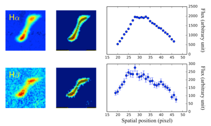
Figure 3.— Left to right, emission line cutout, thresholded emission and total flux as a function of spatial position for H$\alpha$ (top) and H$\beta$ (bottom) of an example galaxy. Yellow stars over plotted on thresholded emission show peaks of Gaussians at each spatial position.

We measure nebular dust attenuation along the disk of the galaxies using the ratio of the first two Balmer transitions ($H\alpha$ and $H\beta$) or the so-called Balmer decrement. Ratio of the luminosities of Balmer transitions arising from HII regions around very massive stars is known to be the most practical indicator measuring attenuation by dust in these regions. In the absence of dust, the intrinsic theoretical H$\alpha$ to H$\beta$ line ratio, assuming Case B recombination, a temperature of $T=10^{4}K$, and an electron density of $n_{e}=10^{2}$ $\rm cm^{-3}$ is known ($F(H\alpha)/F(H\beta)=2.86$; Osterbrock 1989). Any deviation from this amount is indicative of the amount of dust attenuation. We model the line emission at each spatial resolution element of continuum subtracted DEIMOS spectra. We convert the H$\alpha$ to H$\beta$ line ratio at each spatial resolution to an extinction measure using:

$$E(B-V)_{nebular}=\rm\frac{-2.5}{k(H\beta)-k(H\alpha)}log_{10}(\frac{2.86}{H\alpha/H\beta})$$ (1)

We use the Cardelli Galactic extinction curve (Cardelli et al. 1989) for measuring $\rm k(H\beta)$ and $\rm k(H\alpha)$. A line-of-sight attenuation curve such as Cardelli, is more appropriate for recombination emission of compact HII regions compared to more extended stellar continuum attenuation curves such as Calzetti et al. (2000). The latter would cause smaller $E(B-V)_{nebular}$ values by a factor of 0.9 (see Reddy et al. 2015 for a more detailed discussion).

We model and subtract the continuum by first making cutouts of $\sim 100$ Å around the emission line (H$\alpha$ or H$\beta$ in this case). We mask the wavelength range ($\sim 15-20$ Å) where we have the emission in the cutout and bin the rest of the spectra in the wavelength direction with bins of $\sim 5$ Å. The median values in each wavelength bin are then fitted with a Gaussian function in the spatial direction. We measure the continuum under emission by interpolating these values over the masked wavelength range and subtract this continuum from the cutout spectra to have the continuum free emission line.

To model the line emission at each spatial resolution in the galaxy, we make small cutouts covering only the emission from the continuum subtracted spectra. To be able to trace the emission to furthest points from the center and to avoid tracing and fitting the noise in the background, we use the Otsu method (Otsu 1979). Otsu method is an unsupervised automatic thresholding algorithm which reduces a grey level image to a binary image by finding an optimum threshold to maximize the separability of the two classes. Here, using this method we separate the emission from the noise in the background by multiplying the binary image by the continuum subtracted cutout. We fitted Gaussian functions to the emission at each spatial resolution (in the wavelength/velocity direction) to measure the total flux from that resolution element. In figure 3, we show H$\alpha$ and H$\beta$ cutouts as well as the thresholded cutout and traced emission for one example galaxy. We have centered emission lines by the spectroscopic redshift, which comes from visually aligning all the emission lines. However, in order to measure the ratio of two lines we need to be more precise in centering the emissions. We center each emission line by fitting the peak of modeled Gaussians with an arctangent function (in the spatial direction) this takes care of velocity offsets due to rotation in the disk. We measure a correction factor from standard stars to account for flux calibration. This is an essential step even though we are only using the ratio of emission lines, due to the large difference between wavelength of H$\alpha$ and H$\beta$ and the wavelength dependence of flux calibration. This is a factor of $\sim 1.2-1.5$ from $z=0.32-0.47$. The Balmer decrement is then measured along the major axis of galaxies by setting a minimum signal-to-noise ratio (S/N) of 5 and 3 at each spatial resolution for H$\alpha$ and H$\beta$ lines respectively and then dividing the two. Nebular color excess ($E(B-V)_{nebular}$) along the disk is then calculated by the conversion in equation 1. The uncertainty in this ratio is calculated by the standard error propagation method using the H$\alpha$ and H$\beta$ flux uncertainties at each spatial position. In the resolved line measurement, we did not correct for the Balmer absorption because the corrections are very small and well within the uncertainty of the line measurements. Extinction uncertainties range from 0.03-0.2 magnitude and its variation is larger between galaxies compared to that of one single galaxy.

We also measure the integrated or “global” Balmer decrement and nebular color excess values for the whole galaxy by extracting the 1D spectra and measuring line fluxes. We correct our measurements for the underlying Balmer absorption using the stellar population model fits. The corrections to the H$\alpha$ to H$\beta$ ratio are $\lesssim 4\%$. For simplicity, we refer to our dust measurements at each spatial distance from the center as resolved dust measurement.

5. Results

5.1. Color Excess, Stellar Continuum vs. ionized gas

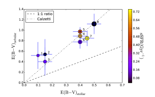
Figure 4.— Integrated nebular color excess of galaxies in the sample measured through the Balmer decrement compared to their stellar color excess measured through SED fitting. Nebular to stellar color excess ratio of 1 and 2.27 (Calzetti et al. 2000) are shown with dashed and dotted-dashed lines respectively. Galaxies are color coded based on their sSFR and symbol size increases with stellar mass.

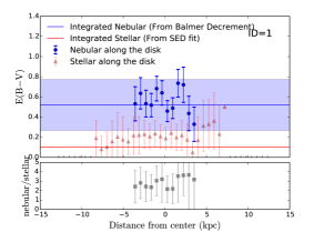
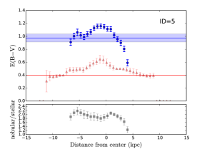
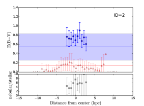
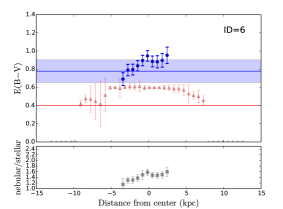
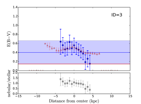
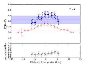
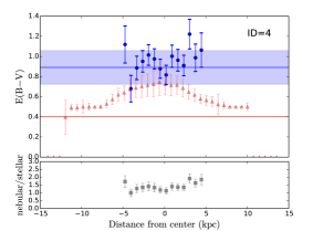
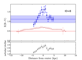
Figure 5.— Nebular and stellar color excess profiles (top panels) and nebular to stellar color excess ratios (bottom panels) along the major axis of galaxies in our sample shown with blue circles and red triangles respectively as a function of distance from the center of galaxies. Blue and red solid lines show the nebular and stellar integrated color excess measured in each galaxy and the blue shaded region is the $1\sigma$ uncertainty in the integrated nebular color excess.

The ratio of the nebular to stellar dust extinction has been studied extensively over the past decade. Studies of local star forming galaxies (e.g. Calzetti et al. 2000; Wild et al. 2011) have found larger attenuation towards the nebular regions compared to the stellar continuum. However, in almost all of these works, there is a large scatter in the nebular vs. stellar color excess relation. Recent works (Reddy et al. 2015) have attributed the scatter in this relation, seen in samples of higher redshift star-forming galaxies, to physical properties of galaxies, specifically their stellar mass or sSFR.

In Figure 4, we compare the integrated nebular and stellar color excesses of galaxies in our sample. We have color-coded our galaxies based on their sSFR and the symbol sizes increase with stellar mass. All our galaxies sit above the $1:1$ (dashed line) nebular to stellar color excess ratio, which means there is larger amount of nebular extinction compared to the continuum. While we do not find any clear trend in this ratio with neither sSFR or stellar mass, the sample size is too small to draw any strong conclusions.

We now compare resolved stellar and nebular attenuation measures along the disk of galaxies (as explained in the previous section). Plotted in Figure 5, are nebular (blue circles) and stellar (red triangles) color excess as a function of distance (in kpc) from the center of the galaxy, as well as the global measurement for each galaxy (solid lines). An agreement is seen among the nebular measurements at the resolution elements with the global measured value for each galaxy. The difference between the median of the measured points and the integrated value in each galaxy ranges from zero to maximum of 0.1 magnitude (well within the uncertainty of the integrated value of each galaxy). The small offset towards higher median values, might be due to the S/N criteria which affects the spectra of the outer parts of the disk more than the central parts. The uncertainties in the measured values become considerably smaller in galaxies with larger stellar masses (the right panels). Almost all the galaxies show higher stellar continuum extinction in the central regions compared to the outer parts in the disk. This differs from the nebular color excess of the lower mass galaxies ($\rm ID=1-4$) which does not significantly vary as a function of their distance from the center. More massive galaxies ($\rm ID=5-8$) however, show higher nebular extinction towards the central parts of galaxies similar to the stellar continuum color excesses.

As shown in Figure 4, the nebular to stellar color excess ratio, varies from galaxy to galaxy. By examining $\rm ID=5$ and $\rm ID=7$, two galaxies with the most extended emissions, highest S/N ratio, exact same redshift and comparable stellar masses, we see very different ionized to continuum color excess ratio. Between the two galaxies the one with the higher sSFR ($\rm ID=7$) has smaller color excess ratio, consistent with the findings of Price et al. (2014) for higher redshift galaxies but inconsistent with Reddy et al. (2015), and the framework depicted by radiative transfer models (e.g. Charlot & Fall 2000).

An important factor that might be playing a role is the difference in the inclination of these two galaxies. The inclination affects observed physical properties of galaxies and in particular their surface brightness (e.g. Holmberg 1958). Many studies used inclination and surface brightness to measure the amount of extinction in disky galaxies (e.g. Giovanelli et al. 1995, Peletier & Willner 1992), knowing that with the same surface brightness, the more inclined galaxy suffers more from dust extinction. More recent study by Yip et al. (2010), confirmed the result of higher stellar extinction in more inclined galaxies using a large sample of local SDSS disk galaxies. More interestingly, this study showed that the amount of the Balmer decrement stays constant with inclination. If true, this can explain some of the dispersion in the ionized vs. stellar dust extinction studies. In the case of this study, if the more inclined galaxy ($\rm ID=7$) were face-on, it would have had less stellar continuum color excess and therefore larger ratio of ionized to stellar color excess similar to the other galaxy ($\rm ID=5$).

We do not find any significant correlation between the nebular to stellar color excess ratio and distance from the center of galaxies (see bottom panels of figure 5) except for the most massive galaxy ($\rm ID=8$) in which this ratio decreases with distance from the center. This is because the resolution of boxes in which the color excess is measured is still significantly larger compared to the sizes of original clouds (sub-kpc) producing the recombination lines. However, future telescopes such as Thirty Meter Telescope (TMT) equipped with integral field unit (IFU) technology and assisted by adaptive optics (AO) systems will be able to provide us with a wealth of information on these clouds at these redshifts.

5.2. Variation of Color Excess with Stellar Mass Surface Density

The typical dust extinction of a galaxy has been shown to depend upon different properties of the galaxy, most fundamentally on its stellar mass (e.g. Garn & Best 2010, Sobral et al. 2012, Ibar et al. 2013). Here, we investigate the variation of color excess in galaxies as a function of the stellar mass surface density at each resolution element along the major axis of the disks.

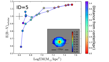
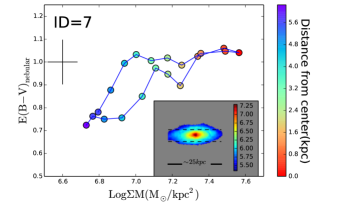
Figure 6.— Variation of nebular color excess as a function of stellar mass surface density in two of the galaxies, at the same redshift and with the same stellar mass. The stellar mass surface density maps are plotted in the corner right of each plot with the DEIMOS slit coverage over plotted. The measurements at each resolution element in the disk are color coded based on their distance from the center (distance from the center decreases going from blue to red color). Average uncertainty in measurements is shown in top left of each panel.

Figure 6, shows the color excess of the ionized gas as a function of stellar mass surface density for two of the galaxies. The data points are color-coded based on their distance from the center and the typical error bars are shown in the top-left corner of each panel. The stellar mass surface density maps from the resolved SED fitting are shown in the lower right part of each plot and over plotted with dashed black lines are the DEIMOS slit position and coverage. It is important to note that while the size of the disk’s major axis is about 20 kpc in these galaxies, the extent of the emission lines is only about 12 kpc. This can be either due to lack of strong emission at large distances in these galaxies, or due partly to the over subtraction of background in larger radii in the DEIMOS reduction pipeline.

It is clear from figure 6 that the color excess of ionized gas is increasing from the outskirts towards the bulge of the galaxies symmetrically, similar to the stellar mass. Putting all the resolution elements of all galaxies in the sample together on the color excess vs. stellar mass surface density plot in Figure 7, we see the overall increase of the median of color excess in bins of stellar mass surface density.

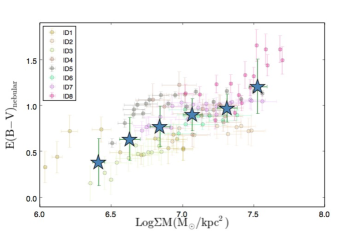
Figure 7.— Variation of color excess as a function of stellar mass surface density in all resolution elements of the galaxies in the sample. Different colors correspond to different galaxies. There is an overall increasing trend of color excess with increasing stellar mass surface density clear from the median represented with blue stars.

5.3. Dust to Gas Ratio

A tight correlation exists between the mean surface density of cold gas and the average SFR per unit area (the so-called SFR law) on global scales (e.g. Kennicutt 1998) as well as on resolved kpc-scales (Kennicutt et al. 2007). This relation (“KS relation”) is parameterized using a power-law introduced by Schmidt (1963). Here, we convert our SFR surface density ($\Sigma_{SFR}$; in units of $\rm M_{\odot}yr^{-1}kpc^{-2}$) measurements to total gas (molecular and atomic) surface density ($\Sigma_{H}$; in units of $\rm M_{\odot}pc^{-2}$), using:

$$\rm log\Sigma_{SFR}=(1.56\pm 0.04)log\Sigma_{H}-(4.32\pm 0.09)$$ (2)

derived by Kennicutt et al. (2007) using observations of the nearby spiral galaxy M51a. We note that as the gas surface densities in higher redshift star forming galaxies is larger compared to M51, using the KS relation is an extrapolation when dealing with high gas surface densities. There are only limited observations of local galaxies with high gas surface densities, and they show evidence of shift in the KS relation at higher redshifts Hodge et al. 2015. Figure 8 shows the variation of nebular color excess per resolution elements along the major axis of galaxies in our sample as a function of gas surface density. There is an increasing trend of color excess with gas surface density at ($log\Sigma_{H}\gtrsim 2.5$). We formalize this relation by fitting a third order polynomial to $E(B-V)_{nebular}$ versus $x\equiv log\Sigma_{H}$ (shown in Figure 8 with magenta dashed line).

$$E(B-V)_{nebular}=0.51x^{3}-3.53x^{2}+7.98x-5.21$$ (3)

It is important to note again that, the sample size is small and we might be missing a population of galaxies that could alter this fit. In figure 8, we over plot the relation of nebular color excess as a function of dust mass surface density (multiplied by a factor of hundred) derived by Kreckel et al. (2013), from resolved FIR (Herschel and Spitzer) and optical integral field observations of a sample of eight nearby disk galaxies. The nebular color excess versus dust mass surface density relation introduced by Kreckel et al. (2013) (solid cyan line in Figure 8 ), is well bracketed by the two extremes of dust geometry discussed in Calzetti et al. (1994) (a uniform foreground dust screen model and a mixed media model), suggesting a combination of the two effects. The shape of the color excess versus dust mass surface density resembles that with gas surface density at higher gas surface densities. This implies that the change in the dust to gas ratio is insignificant in these regions with different amounts of extinction, while this is not the case at lower gas mass surface densities. Many previous studies have assumed a fixed dust to gas ratio in galaxies (e.g. Leroy et al. 2011, Sandstrom et al. 2013), this result certifies the fairness of those assumption at high gas mass surface densities. The difference in the lower gas mass surface densities, however is suggestive of a variable gas to dust ratio.

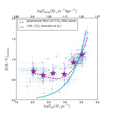
Figure 8.— Variation of nebular color excess as a function of gas surface density in all resolution elements of the galaxies in the sample. Magenta stars show the median in bins of gas surface density and the magenta dashed line is a third order polynomial fit to blue data points. Cyan solid line shows the relation between the nebular E(B-V) and dust mass surface density (multiplied by a factor of 1500), from Kreckel et al. (2013).

6. Summary and Discussion

In this work, we have measured resolved kpc-scale dust reddening along the major axis of eight emission-line disky galaxies at $z\sim 0.4$. We have used pixel-by-pixel SED fitting and Keck/DEIMOS spectra to infer stellar and nebular dust extinction at kpc-scales, respectively. While the sample size redshift range probed are small to draw robust statistical inferences about galaxy populations in general, we developed the methodology that can be practically used on much larger samples to measure dust inside galaxies at different radii from the center, using optical spectra from local galaxies to $z\sim 0.5$ and infrared spectra at higher redshifts. These kind of studies could then be used to address the variation of results for integrated galaxies at high-z found in the literature.

The integrated nebular to stellar color excess ratio for the galaxies in our sample are larger than unity with median $(E(B-V)_{nebular}/E(B-V)_{stellar})=2.5$ and standard deviation $1.0$. Due to the small sample size a clear trend of nebular to stellar color excess ratio was not seen with either stellar mass or the sSFR. However the nebular to stellar color excess ratio dependence can be investigated for individual galaxies. We specifically compared two of the galaxies in the sample ($\rm ID=5\&7$) with the same redshift ($z=0.38$) and comparable stellar mass ($Log(M_{*}/M_{\odot}\sim 9.65$). Between the two, the one with higher SFR has smaller nebular to stellar color excess ratio. This is in agreement with the work of Price et al. (2014) but contrary to the overall trend seen in Reddy et al. 2015 with integrated measurements for larger samples of galaxies at higher redshifts. The difference here can be explained due to differences in the orientations (inclinations) between the two galaxies, a parameter that is often overlooked in many studies.

We also compared the integrated and resolved nebular color excess in galaxies and found a good agreement between the two, with the integrated value, being equal or slightly less than the median of resolved measurements (median $\Delta E(B-V)_{median-integrated}\sim 0.05$ mag). This small offset is mostly due to the signal to noise criteria applied to H$\alpha$ and H$\beta$ emission lines at resolution elements, which exclude the outer parts of the emission line (which also appear to have lower extinction) from the resolved measurements. We found that the resolved stellar continuum color excess profiles show higher extinction towards central regions of galaxies compared to outer parts of the disk. This is contrary the nebular color excess profiles in the lower mass galaxies which show almost flat radial profiles.

The relation between the stellar mass and color excess has been studied at various redshifts (e.g. Garn & Best 2010, Sobral et al. 2012, Domínguez et al. 2013). Here, we extended this relation to substructures inside galaxies, by studying the variation of nebular color excess as a function of stellar mass surface density and found an increasing amount of nebular color excess in regions with higher stellar mass surface density. This also explains to some extent, the lack of a correlation in the nebular attenuation as a function of distance from the center in lower mass galaxies in which the stellar mass surface density range covered is lower, when compared to higher mass galaxies.

We also examined the relation between the nebular color excess and the gas mass surface densities, converted from the SFR surface densities. The shape of the attenuation relation for high gas mass surface densities resembles the attenuation versus dust mass surface density relation found in Kreckel et al. (2013), implying that the dust to gas mass ratio is not changing significantly as a function of extinction at physical scale probed in this study. It is however important to note the assumptions made in deriving this result, such as the conversion from SFR surface density to gas surface density and the dust mass surface densities which are all measured from local observations and might not hold true at higher redshifts. Resolved FIR observations with the Atacama Large Millimeter/submillimeter Array (ALMA) will be essential to examine the validity of these assumptions.

References

- Abazajian et al. (2009) Abazajian, K. N., Adelman-McCarthy, J. K., Agüeros, M. A., et al. 2009, ApJS, 182, 543
- Arnouts et al. (1999) Arnouts, S., Cristiani, S., Moscardini, L., et al. 1999, MNRAS, 310, 540
- Asari et al. (2007) Asari, N. V., Cid Fernandes, R., Stasińska, G., et al. 2007, MNRAS, 381, 263
- Bertin & Arnouts (1996) Bertin, E., & Arnouts, S. 1996, A&AS, 117, 393
- Boquien et al. (2011) Boquien, M., Calzetti, D., Combes, F., et al. 2011, AJ, 142, 111
- Bruzual & Charlot (2003) Bruzual, G., & Charlot, S. 2003, MNRAS, 344, 1000
- Bundy et al. (2005) Bundy, K., Ellis, R. S., & Conselice, C. J. 2005, ApJ, 625, 621
- Calzetti (2001) Calzetti, D. 2001, PASP, 113, 1449
- Calzetti et al. (2000) Calzetti, D., Armus, L., Bohlin, R. C., et al. 2000, ApJ, 533, 682
- Calzetti et al. (1994) Calzetti, D., Kinney, A. L., & Storchi-Bergmann, T. 1994, ApJ, 429, 582
- Cardelli et al. (1989) Cardelli, J. A., Clayton, G. C., & Mathis, J. S. 1989, ApJ, 345, 245
- Chabrier (2003) Chabrier, G. 2003, PASP, 115, 763
- Charlot & Fall (2000) Charlot, S., & Fall, S. M. 2000, ApJ, 539, 718
- Curtis (1918) Curtis, H. D. 1918, PASP, 30, 65
- Domínguez et al. (2013) Domínguez, A., Siana, B., Henry, A. L., et al. 2013, ApJ, 763, 145
- Erb et al. (2006) Erb, D. K., Steidel, C. C., Shapley, A. E., et al. 2006, ApJ, 647, 128
- Faber et al. (2003) Faber, S. M., Phillips, A. C., Kibrick, R. I., et al. 2003, in Society of Photo-Optical Instrumentation Engineers (SPIE) Conference Series, Vol. 4841, Instrument Design and Performance for Optical/Infrared Ground-based Telescopes, ed. M. Iye & A. F. M. Moorwood, 1657–1669
- Förster Schreiber et al. (2009) Förster Schreiber, N. M., Genzel, R., Bouché, N., et al. 2009, ApJ, 706, 1364
- Garn & Best (2010) Garn, T., & Best, P. N. 2010, MNRAS, 409, 421
- Genzel et al. (2010) Genzel, R., Tacconi, L. J., Gracia-Carpio, J., et al. 2010, MNRAS, 407, 2091
- Giavalisco et al. (2004) Giavalisco, M., Ferguson, H. C., Koekemoer, A. M., et al. 2004, ApJ, 600, L93
- Giovanelli et al. (1995) Giovanelli, R., Haynes, M. P., Salzer, J. J., et al. 1995, AJ, 110, 1059
- Gordon et al. (2003) Gordon, K. D., Clayton, G. C., Misselt, K. A., Landolt, A. U., & Wolff, M. J. 2003, ApJ, 594, 279
- Grogin et al. (2011) Grogin, N. A., Kocevski, D. D., Faber, S. M., et al. 2011, ApJS, 197, 35
- Guo et al. (2015) Guo, Y., Ferguson, H. C., Bell, E. F., et al. 2015, ApJ, 800, 39
- Hemmati et al. (2014) Hemmati, S., Miller, S. H., Mobasher, B., et al. 2014, ApJ, 797, 108
- Hodge et al. (2015) Hodge, J. A., Riechers, D., Decarli, R., et al. 2015, ApJ, 798, L18
- Holmberg (1958) Holmberg, E. 1958, Meddelanden fran Lunds Astronomiska Observatorium Serie II, 136, 1
- Ibar et al. (2013) Ibar, E., Sobral, D., Best, P. N., et al. 2013, MNRAS, 434, 3218
- Ilbert et al. (2006) Ilbert, O., Arnouts, S., McCracken, H. J., et al. 2006, A&A, 457, 841
- Ilbert et al. (2008) Ilbert, O., Salvato, M., Capak, P., et al. 2008, in Astronomical Society of the Pacific Conference Series, Vol. 399, Panoramic Views of Galaxy Formation and Evolution, ed. T. Kodama, T. Yamada, & K. Aoki, 169
- Kennicutt (1998) Kennicutt, Jr., R. C. 1998, ApJ, 498, 541
- Kennicutt et al. (2007) Kennicutt, Jr., R. C., Calzetti, D., Walter, F., et al. 2007, ApJ, 671, 333
- Koekemoer et al. (2011) Koekemoer, A. M., Faber, S. M., Ferguson, H. C., et al. 2011, ApJS, 197, 36
- Kreckel et al. (2013) Kreckel, K., Groves, B., Schinnerer, E., et al. 2013, ApJ, 771, 62
- Kriek & Conroy (2013) Kriek, M., & Conroy, C. 2013, ApJ, 775, L16
- Kriek et al. (2015) Kriek, M., Shapley, A. E., Reddy, N. A., et al. 2015, ApJS, 218, 15
- Leroy et al. (2011) Leroy, A. K., Bolatto, A., Gordon, K., et al. 2011, ApJ, 737, 12
- Ly et al. (2012) Ly, C., Malkan, M. A., Kashikawa, N., et al. 2012, ApJ, 757, 63
- Miller et al. (2011) Miller, S. H., Bundy, K., Sullivan, M., Ellis, R. S., & Treu, T. 2011, ApJ, 741, 115
- Moustakas & Kennicutt (2006) Moustakas, J., & Kennicutt, Jr., R. C. 2006, ApJ, 651, 155
- Oke & Gunn (1983) Oke, J. B., & Gunn, J. E. 1983, ApJ, 266, 713
- Osterbrock (1989) Osterbrock, D. E. 1989, Astrophysics of gaseous nebulae and active galactic nuclei
- Oteo et al. (2015) Oteo, I., Sobral, D., Ivison, R. J., et al. 2015, ArXiv e-prints, arXiv:1506.02670
- Otsu (1979) Otsu, N. 1979, Systems, Man and Cybernetics, IEEE Transactions on, 9, 62
- Pannella et al. (2009) Pannella, M., Carilli, C. L., Daddi, E., et al. 2009, ApJ, 698, L116
- Peletier & Willner (1992) Peletier, R. F., & Willner, S. P. 1992, AJ, 103, 1761
- Prevot et al. (1984) Prevot, M. L., Lequeux, J., Prevot, L., Maurice, E., & Rocca-Volmerange, B. 1984, A&A, 132, 389
- Price et al. (2014) Price, S. H., Kriek, M., Brammer, G. B., et al. 2014, ApJ, 788, 86
- Reddy et al. (2010) Reddy, N. A., Erb, D. K., Pettini, M., Steidel, C. C., & Shapley, A. E. 2010, ApJ, 712, 1070
- Reddy et al. (2015) Reddy, N. A., Kriek, M., Shapley, A. E., et al. 2015, ArXiv e-prints, arXiv:1504.02782
- Sandstrom et al. (2013) Sandstrom, K. M., Leroy, A. K., Walter, F., et al. 2013, ApJ, 777, 5
- Schmidt (1963) Schmidt, M. 1963, ApJ, 137, 758
- Scoville et al. (2015) Scoville, N., Faisst, A., Capak, P., et al. 2015, ApJ, 800, 108
- Shivaei et al. (2015) Shivaei, I., Reddy, N. A., Steidel, C. C., & Shapley, A. E. 2015, ApJ, 804, 149
- Sobral et al. (2012) Sobral, D., Best, P. N., Matsuda, Y., et al. 2012, MNRAS, 420, 1926
- Sobral et al. (2013) Sobral, D., Swinbank, A. M., Stott, J. P., et al. 2013, ApJ, 779, 139
- Stecher (1965) Stecher, T. P. 1965, ApJ, 142, 1683
- Sullivan et al. (2001) Sullivan, M., Mobasher, B., Chan, B., et al. 2001, ApJ, 558, 72
- Swinbank et al. (2012) Swinbank, A. M., Sobral, D., Smail, I., et al. 2012, MNRAS, 426, 935
- Wang & Heckman (1996) Wang, B., & Heckman, T. M. 1996, ApJ, 457, 645
- Wild et al. (2011) Wild, V., Charlot, S., Brinchmann, J., et al. 2011, MNRAS, 417, 1760
- Wisnioski et al. (2015) Wisnioski, E., Förster Schreiber, N. M., Wuyts, S., et al. 2015, ApJ, 799, 209
- Wuyts et al. (2011) Wuyts, S., Förster Schreiber, N. M., van der Wel, A., et al. 2011, ApJ, 742, 96
- Wuyts et al. (2012) Wuyts, S., Förster Schreiber, N. M., Genzel, R., et al. 2012, ApJ, 753, 114
- Wuyts et al. (2013) Wuyts, S., Förster Schreiber, N. M., Nelson, E. J., et al. 2013, ApJ, 779, 135
- Yip et al. (2010) Yip, C.-W., Szalay, A. S., Wyse, R. F. G., et al. 2010, ApJ, 709, 780