Constraints on the Intergalactic Magnetic Field with Gamma-Ray Observations of Blazars

Abstract

Distant BL Lacertae objects emit $\gamma$ rays which interact with the extragalactic background light (EBL), creating electron-positron pairs, and reducing the flux measured by ground-based imaging atmospheric Cherenkov telescopes (IACTs) at very-high energies (VHE). These pairs can Compton-scatter the cosmic microwave background, creating a $\gamma$-ray signature at slightly lower energies observable by the Fermi Large Area Telescope (LAT). This signal is strongly dependent on the intergalactic magnetic field (IGMF) strength ($B$) and its coherence length ($L_{B}$). We use IACT spectra taken from the literature for 5 VHE-detected BL Lac objects, and combine it with LAT spectra for these sources to constrain these IGMF parameters. Low $B$ values can be ruled out by the constraint that the cascade flux cannot exceed that observed by the LAT. High values of $B$ can be ruled out from the constraint that the EBL-deabsorbed IACT spectrum cannot be greater than the LAT spectrum extrapolated into the VHE band, unless the cascade spectrum contributes a sizable fraction of the LAT flux. We rule out low $B$ values ($B\lesssim 10^{-19}$ G for $L_{B}\geq 1$ Mpc) at $>5\sigma$ in all trials with different EBL models and data selection, except when using $>1\ \mathrm{GeV}$ spectra and the lowest EBL models. We were not able to constrain high values of $B$.

1. Introduction

The extragalactic background light (EBL) from the infrared (IR), through the optical and into the ultraviolet (UV) is dominated by emission from all the stars in the observable universe, either directly or through dust absorption and reradiation. It contains information about the cosmological expansion, star formation history, dust extinction and radiation in the universe, and so can provide constraints on a number of cosmologically interesting parameters. However, its direct detection is hampered by the bright foreground emission from the Earth’s atmosphere, the solar system, and the Galaxy. This can be avoided by making measurements from spacecraft outside the Earth’s atmosphere (e.g., Hauser et al., 1998; Dwek et al., 1998; Bernstein et al., 2002; Mattila, 2003; Bernstein, 2007) or solar system (Toller, 1983; Leinert et al., 1998; Edelstein et al., 2000; Murthy et al., 2001; Matsuoka et al., 2011), or through galaxy counts, which in general give lower limits (e.g., Madau & Pozzetti, 2000; Marsden et al., 2009). See for example Hauser & Dwek (2001) for a review of EBL measurements, constraints, and models.

Shortly after the discovery of the cosmic microwave background (CMB) radiation (Penzias & Wilson, 1965), it was realized that this and other radiation fields would interact with extragalactic $\gamma$ rays, producing electron-positron pairs, effectively absorbing the $\gamma$ rays (Nikishov, 1962; Gould & Schréder, 1967; Fazio & Stecker, 1970). In the 1990s, extragalactic high-energy $\gamma$-ray astronomy took major leaps forward, with the launch of the Compton Gamma-Ray Observatory and the first detections of extragalactic sources at high energies (MeV–GeV) by EGRET (Hartman et al., 1992), and at very-high energies (VHE; $\gtrsim 0.1$ TeV) by ground-based imaging atmospheric Cherenkov telescopes (IACTs; Punch et al., 1992; Mohanty et al., 1993). It was almost immediately realized that $\gamma$-ray observations of extragalactic blazars could be used to constrain the EBL (Stecker et al., 1992; Stecker & de Jager, 1993; Dwek & Slavin, 1994; Biller et al., 1995; Madau & Phinney, 1996). The detection of Mrk 501 out to 20 TeV (Aharonian et al., 1999) was not consistent with the EBL models of the time (Aharonian et al., 1999; Protheroe & Meyer, 2000). The detection of the hard spectrum from the BL Lac 1ES 1101$-$232 with H.E.S.S. seems to put strong constraints on the EBL, ruling out models that predict high opacity if one assumes the intrinsic VHE spectrum cannot be harder than $\Gamma=1.5$, where the differential photon flux $\Phi(E)=dN/dE\propto E^{-\Gamma}$ (Aharonian et al., 2006). However, the $\Gamma=1.5$ constraint has been questioned, and a number of theoretical possibilities have been raised that could account for harder VHE spectra (Stecker, Baring, & Summerlin, 2007; Böttcher, Dermer, & Finke, 2008; Aharonian, Khangulyan, & Costamante, 2008). Nonetheless, the basic idea, that the deabsorbed VHE photon index cannot be harder than a certain value, has been used by many authors to constrain the EBL (e.g., Schroedter, 2005; Aharonian et al., 2007d; Mazin & Raue, 2007; Albert et al., 2008; Finke & Razzaque, 2009). EBL constraints from $\gamma$-ray observations have been used to constrain the contribution of Population II and III stars to the EBL star formation (Raue et al., 2009; Raue & Meyer, 2012; Gilmore, 2012), including the contribution of dark matter-powered stars (Maurer et al., 2012).

The new era of $\gamma$-ray astronomy, which has begun with the launch of the Fermi Gamma-Ray Space Telescope has brought additional constraints on the EBL. The Fermi Large Area Telescope (LAT) is sensitive to $\gamma$ rays from 20 MeV to greater than 300 GeV (Atwood et al., 2009) and surveys the entire sky every $\sim$ 3 hours, collecting an unprecedented number of $\gamma$-ray photons from the entire sky. At the energies observed by the LAT, the extragalactic $\gamma$-ray sky below $\sim$ 10 GeV is expected to be entirely transparent to $\gamma$ rays, at least back to the era of recombination ($z\sim 1000$) (e.g., Oh, 2001; Finke et al., 2010), while photons observed in the 10 GeV – 300 GeV range should be attenuated by UV/optical photons if they originate from sources at $z\gtrsim 0.5$. This suggests a possible way to constrain the EBL (Chen, Reyes, & Ritz, 2004). The LAT spectrum below 10 GeV can be extrapolated to higher energies, and should be an upper limit on the intrinsic spectrum in the range where the EBL attenuates the $\gamma$ rays. This seems to be a reasonable assumption, since no spectrum that contradicts this has been observed, and it is difficult to imagine theoretical ways to produce one, although see e.g. Aharonian et al. (2002, 2008); Lefa et al. (2011). Abdo et al. (2010) have used this technique to put upper limits on the optical/UV EBL absorption optical depth ($\tau_{\gamma\gamma}$) for sources $z\gtrsim 0.5$, and rule out with high significance some models which predict high $\tau_{\gamma\gamma}$ with data from the first 11 months of LAT operation from 5 blazars and 2 gamma-ray bursts (GRBs). More recently, Ackermann et al. (2012) used a similar technique in a composite fit to 150 BL Lacs with 46 months of LAT data to constrain the high-$z$ EBL even further, and found agreement with most recent models (Franceschini et al., 2008; Gilmore et al., 2009; Finke et al., 2010; Kneiske & Dole, 2010; Domínguez et al., 2011; Gilmore et al., 2012). Abramowski et al. (2013) performed a combined analysis of HESS blazar spectra and found them to be consistent with EBL absorption using the model of Franceschini et al. (2008). Georganopoulos et al. (2008) suggested the Compton-scattering of EBL photons by high-energy electrons in the radio lobes of Fornax A could be detected by the Fermi-LAT, leading to another possible way to constrain EBL intensity.

Below 100 GeV, the universe is expected to be transparent out to $z\sim 0.1$, although VHE photons from this redshift range should be attenuated by interactions with IR EBL photons. Georganopoulos, Finke, & Reyes (2010) suggested a very similar technique to Abdo et al. (2010), applied to the VHE range. For those sources detected by both LAT and an IACT, one can extrapolate the LAT spectrum (which should be unattenuated for these sources at low $z$) into the VHE range, and use it as an upper limit on the intrinsic VHE flux. As with the LAT-only case, a comparison of this upper limit with the observed VHE flux allows one to compute an upper limit on $\tau_{\gamma\gamma}$. Georganopoulos et al. (2010) used this technique to show that models which predicted high $\tau_{\gamma\gamma}$ in the VHE range were strongly disfavored. Another possible way to estimate the intrinsic spectrum of a source, and thus estimate $\tau_{\gamma\gamma}$, comes from modeling the full radio to GeV $\gamma$-ray spectral energy distribution (SED) of a $\gamma$-ray blazar with a standard synchrotron/synchrotron self-Compton (SSC) model. The SSC spectrum can be extrapolated to the VHE regime, and compared with observations to estimate $\tau_{\gamma\gamma}$ (Mankuzhiyil et al., 2011). Domínguez et al. (2013) have applied this technique to a sample of $\sim 15$ LAT and IACT-detected blazars to constrain the cosmic $\gamma$-ray horizon, i.e., the energy where $\tau_{\gamma\gamma}=1$ for a certain redshift. Dwek & Krennrich (2013) present a comprehensive review of recent attempts to constrain the EBL with $\gamma$-ray observations.

These constraints come with caveats, however. A major one is that the GeV and VHE $\gamma$ rays must come from the same region in the jet. But the VHE $\gamma$ rays could have a different origin: namely, they could be created in a different region of the jet (Böttcher et al., 2008), or from ultra-high energy cosmic rays (UHECRs) which originate from the blazar, and interact with the CMB and IR-UV EBL to produce VHE $\gamma$ rays (Essey & Kusenko, 2010; Essey et al., 2010, 2011b; Razzaque et al., 2012). Another possibility is that the electrons that are produced by the $\gamma$-ray–EBL photon interactions Compton-scatter CMB photons, producing GeV $\gamma$-ray emission which could itself be absorbed by interactions with the EBL, producing a cascade (Aharonian et al., 1994; Plaga, 1995; Dai et al., 2002). If the intergalactic magnetic field (IGMF) strength is low, the pairs will not be significantly deflected from our line of sight, and this could produce an observable feature in the LAT bandpass (e.g., Neronov & Semikoz, 2009). This cascade component was taken into account in the EBL constraints of Meyer et al. (2012), and could be an important component that should be included in the broadband spectral modeling of BL Lac objects (e.g., Tavecchio et al., 2011; Tanaka et al., 2014). In recent years several authors have used the non-detection of these cascades to put lower limits on the IGMF strength (e.g., Neronov & Vovk, 2010; Tavecchio et al., 2010; Dolag et al., 2011; Essey et al., 2011a). In general these efforts depend on the fact that emission from VHE blazars is relatively constant over long periods of time ($\gtrsim 10^{6}$ years). Some VHE blazars have been seen to have non-variable emission on timescales of years (e.g., Aharonian et al., 2006, 2007d), but other blazars are highly variable at these energies (e.g., Aharonian et al., 2007a). Indeed observing and studying the time-dependent EBL-induced pair cascades from GRBs and blazar flares has been suggested as a way to probe the IGMF parameters (Razzaque et al., 2004; Ichiki et al., 2008; Murase et al., 2008). The possibility of variable VHE emission has led to caveats in interpreting the IGMF constraints from apparently non-variable TeV blazars (Dermer et al., 2011; Taylor et al., 2011). Other uncertainties such as the EBL intensity and VHE spectra errors, blazar jet geometry and Doppler factor, can further decrease the lower limits on the IGMF (Arlen et al., 2014). For higher values of the intergalactic magnetic field strength, the cascade emission is not expected to be a point source, so would result in $\gamma$-ray “halos” in the $\sim 0.1$—$100\ \mathrm{GeV}$ energy range around VHE-detected blazars (Neronov & Semikoz, 2009). The detection of these halos was reported by Ando & Kusenko (2010), but it was contested by Neronov et al. (2011) and Ackermann et al. (2013). The cascades might also be suppressed by plasma beam instabilities (Broderick et al., 2012; Schlickeiser et al., 2012a, b; Menzler & Schlickeiser, 2015), although this is controversial (Venters & Pavlidou, 2013; Miniati & Elyiv, 2013; Sironi & Giannios, 2014; Chang et al., 2014).

In this paper we report on our efforts to constrain the IGMF strength ($B_{IG}$) and coherence length ($L_{B}$) using $\gamma$-ray observations of blazars from both LAT and IACTs. This technique can be seen as an extension of previous work by Georganopoulos et al. (2010), where the focus was on constraining the EBL. We make use of data from the first 70 months of LAT operation, the analysis of which is described in Section 2, and IACT spectra from the literature. We describe our technique in section 3 and report on our constraints on IGMF parameters in Section 4. Finally we discuss the interpretations and implications of our results in Section 5.

2. LAT Analysis

To determine the LAT spectra of our sources, listed in Table 1, we considered all LAT data collected since the start of the science mission in 2008 August 4 (MJD 54682) until 2014 June 30 (MJD 56838), i.e. for 70 months of operation. This constitutes a significant increase in statistics with respect to previous efforts (e.g., Neronov & Vovk, 2010; Tavecchio et al., 2010). The data were analyzed using an official release of the Fermi ScienceTools (v9r34p1), 7RE_SOURCE_V15  instrument response functions and considering photons satisfying the

OURCE \ event
selection. We exclude photons detected at instrument zenith angles
greater than 100\arcdeg\ to avoid contamination from the Earth’s limb,
and data taken with the Earth within the LAT’s field of view by
requiring a rocking angle less than 52\arcdeg.
For completeness, we created and used LAT spectra both $>0.1$\ GeV and
$>1.0$\ GeV.  The source 1E

0229$+$200 is significantly contaminated at low energies by albedo gamma-ray emission from the Moon (Johannesson et al., 2013), so for this object we excluded data while the source was near the Sun or Moon (angular distance less than $15^{\circ}$), reducing the exposure by about 10%. For all of our sources, we excluded time intervals around bright gamma-ray bursts and solar flares, as recommended by Acero et al. (2015).

The spectral analysis of each source is based on the maximum likelihood technique using the standard likelihood analysis software. In addition to Galactic and isotropic diffuse background components, we considered all point-like sources within 15° from the source position that we found in the second Fermi catalog (2FGL; Nolan et al., 2012) and a preliminary version of the third Fermi catalog (3FGL, Acero et al., 2015). Sources within $5^{\circ}$ of the source had their normalizations and spectral parameters (i.e., spectral index and log-parabola width parameter if appropriate) free to vary. Sources between $5^{\circ}$ and $10^{\circ}$ had their normalizations free to vary but their spectral parameters fixed to the catalog values. Sources farther than $10^{\circ}$ had their normalizations fixed to their catalog as well. Any residual hotspots in the Test Statistic ($TS$; Mattox et al., 1996) maps with $TS>10$ and less than $10^{\circ}$ from the source were modeled as point sources at the location of the maximum TS value. A likelihood ratio test was used to find the best spectral model (power-law, broken power law, or log parabola) that fit the data. In all cases, there was insufficient evidence to reject the simple power-law model. The power-law spectral parameters resulting from our fits can be found in Table 1, including the $TS$, total photon flux ($F_{LAT}$), spectral index ($\Gamma$), and the off-diagonal term in the covariance matrix (${\rm cov}(F_{LAT},\Gamma)=\sigma_{F}\sigma_{\Gamma}\rho$; e.g., Abdo et al., 2009). Using the off-diagonal terms in the covariance matrix insures that we take into account the correlation between the errors in the parameters $F_{LAT}$ and $\Gamma$ in our error analysis, described in Section 3.3.

In addition to the standard maximum likelihood analysis performed to find the best fit to the data, the Log-of-the-likelihood ($LL$) profile as a function of the source’s photon flux ($F_{LAT}$) was calculated in order to fully characterize the uncertainty on this parameter. While stepping through the source’s flux, the other parameters, such as the source’s spectral index, the free parameters from nearby sources, and the normalizations of the diffuse models, were left free to vary. Thus, instead of assuming a perfect normal (Gaussian) distribution for the error of $F_{LAT}$ and using 1, 2, and 3 standard deviations to calculate the 68%, 95% and 99% confidence intervals, we used the $LL$ profile to calculate the actual confidence intervals assuming that $-2\Delta(LL)$ is distributed as the chi-square probability distribution with one degree of freedom. We found that this approach is necessary in order to correctly determine the flux probability distribution of weak LAT sources such as 1ES 0229+200, 1ES 0347$-$121 and 1ES 1101$-$232. See Section 3.4 for the details of the probability distributions used in our Monte Carlo (MC) analysis, which is described in Section 3.3. We also used this technique for the spectral indices and found that their errors are well-represented by normal distributions.

Table 1Sources and results of LAT analysis.

Source name	3FGL name	$z$	VHE instrument	VHE reference	LAT energy range	$TS$	$F_{LAT}$	$\Gamma$	$\rho\sigma_{F}\sigma_{\Gamma}$	$V$
1ES 0229+200 (catalog )	J0232.8+2016	0.139	HESS	Aharonian et al. (2007d)	0.1–300 GeV	58.0	$1.76\pm 0.09$	$1.71\pm 0.16$	0.014	49
1ES 0229+200 (catalog )					1.0–300 GeV	52.4	$0.30\pm 0.08$	$1.62\pm 0.17$	$7.9\times 10^{-3}$
1ES 0347$-$121 (catalog )	J0349.2$-$1158	0.185	HESS	Aharonian et al. (2007c)	0.1–300 GeV	48.8	$1.18\pm 0.49$	$1.66\pm 0.14$	$5.7\times 10^{-3}$	44
1ES 0347$-$121 (catalog )					1.0–300 GeV	50.2	$0.30\pm 0.07$	$1.77\pm 0.17$	$3.9\times 10^{-3}$
1ES 0414+009 (catalog )	J0416.8+0104	0.287	HESS	Abramowski et al. (2012)	0.1–300 GeV	127	$3.10\pm 0.99$	$1.74\pm 0.10$	0.092	56
1ES 0414+009 (catalog )					1.0–300 GeV	127	$0.56\pm 0.09$	$1.73\pm 0.12$	$4.7\times 10^{-3}$
1ES 1101$-$232 (catalog )	J1103.5$-$2329	0.186	HESS	Aharonian et al. (2007b)	0.1–300 GeV	75.6	$1.57\pm 0.67$	$1.63\pm 0.14$	0.084	37
1ES 1101$-$232 (catalog )					1.0–300 GeV	70.3	$0.34\pm 0.08$	$1.59\pm 0.15$	$5.9\times 10^{-3}$
1ES 1218+304 (catalog )	J1221.3+3010	0.182	VERITAS	Acciari et al. (2009)	0.1–300 GeV	1690	$15.6\pm 1.5$	$1.68\pm 0.03$	0.040	92
1ES 1218+304 (catalog )					1.0–300 GeV	1603	$32.3\pm 1.8$	$1.69\pm 0.04$	0.024

3. Method for Constraining Models

3.1. Assumptions

Our technique for constraining the IGMF is based on Georganopoulos et al. (2010), with extensions including a sophisticated MC technique to more accurately determine the significance of the constraints, and the addition of a pair cascade component. We make the following assumptions, the first three of which are identical to those of Georganopoulos et al. (2010):

1. We assume the MeV-TeV flux from BL Lacs in our sample are produced cospatially from the sources themselves and not UHECR interactions in intergalactic space (Essey & Kusenko, 2010), and that the deabsorbed VHE data points never exceed the extrapolated LAT spectra (within errors). The latter is a fairly common assumption made for the purposes of constraining the EBL (e.g., Georganopoulos et al., 2010; Meyer et al., 2012; Sanchez et al., 2013), and we consider it likely, since there is as yet no evidence for concave upwards $\gamma$-ray spectra. In the Third LAT AGN catalog (Ackermann et al., 2015), 131 sources significantly prefer a log-parabola to a power-law spectrum, yet not one has a concave upwards $\gamma$-ray spectrum. See Costamante (2013) for a different opinion of this assumption.

2. We assume the objects are not variable at $\gamma$-ray energies within the statistical uncertainties of the measurements. Indeed, we have selected sources for our sample for which little or no $\gamma$-ray variability has been reported, in either the LAT or IACTs.

3. We assume the $\gamma$ rays will not convert to axion-like particles or avoid absorption via some other exotic mechanism (e.g., de Angelis et al., 2007; Sánchez-Conde et al., 2009; Reesman & Walker, 2014; Meyer et al., 2014) and that their absorption is correctly described by the EBL model used. We use three EBL models, the “Model C” model of Finke et al. (2010), the lower limit model of Kneiske & Dole (2010), and the model of Franceschini et al. (2008).

4. We assume pairs created by $\gamma$-ray-EBL photon interactions will Compton-scatter the CMB, and will lose energy primarily through scattering and not through intergalactic plasma beam instabilities (Broderick et al., 2012; Schlickeiser et al., 2012a, b). Our technique for including the cascade component is similar to the one used by Meyer et al. (2012).

5. We assume the IGMF does not change significantly with redshift. The IGMF strength is expected to be larger at earlier redshift as $B_{IG}\propto(1+z)^{2}$ (Neronov & Semikoz, 2009). For the low redshifts probed in this paper, $z<0.3$, the variation in $B_{IG}$ with redshift will be negligible in comparison with the spacing in our grid of tested values.

6. We assume that all of the cascade flux is produced inside the LAT PSF. It is possible the cascade could be extended as observed by the LAT, due to the pair halo effect (e.g., Neronov & Semikoz, 2009).

We constrain the IGMF in two ways. If the cascade flux resulting from the absorption of VHE $\gamma$ rays exceeds the observed LAT flux, low values of $B_{IG}$ can be ruled out. This technique was used previously by Neronov & Vovk (2010) and others. If $B_{IG}$ is high, the cascade will be minimal. If the deabsorbed VHE points are above the extrapolated LAT spectrum, one could interpret this as ruling out a particular EBL model, as discussed by Georganopoulos et al. (2010). However, this technique neglects the contribution of the cascade flux to the observed LAT emission. So we interpret this constraint as ruling out high $B_{IG}$ values: if the deabsorbed VHE spectral points are above the extrapolated LAT spectrum, it must mean that there is a contribution to the LAT spectrum from the cascade component, so that one cannot know how much of the observed LAT spectrum comes directly from the source. A minimum necessary cascade implies an upper limit on $B_{IG}$.

3.2. Source Selection

We first selected sources which met the following criteria:

• We select blazars that are found in the preliminary version of the 3FGL and in the TeVCat. with a published VHE spectrum and a measured redshift.

• We select sources which have variability index $<100$ in the 3FGL, corresponding to a significance of $4.8\sigma$ that the source is variable. We prefer sources with little variability, since one of our method’s assumptions is that they have little variability (see Section 3.1).

• We restrict ourselves to sources with measured redshift $z\lesssim 0.3$. This is because the cascade calculation we use, from Dermer et al. (2011) and Dermer (2013), is not valid at redshifts $z\gtrsim 0.3$. This excludes some sources which will certainly be very constraining. In particular, PKS 1424+240 (Acciari et al., 2010) has its redshift constrained to $z\gtrsim 0.6$ (Furniss et al., 2013), and could be highly constraining.

• Finally, for the remaining sources, we deabsorbed the VHE spectra with the EBL model of Finke et al. (2010) and plotted them with the LAT spectra, extrapolated into the VHE regime. We chose sources which had deabsorbed VHE spectra above or nearly above their extrapolated LAT spectra (e.g., Figure 1). Although 1ES 1218+304 did not meet this criterion, we included it anyway, because it previously gave strong EBL constraints (Georganopoulos et al., 2010).

Our sources, the details of their LAT spectra, and the sources of their VHE spectra, are given in Table 1.

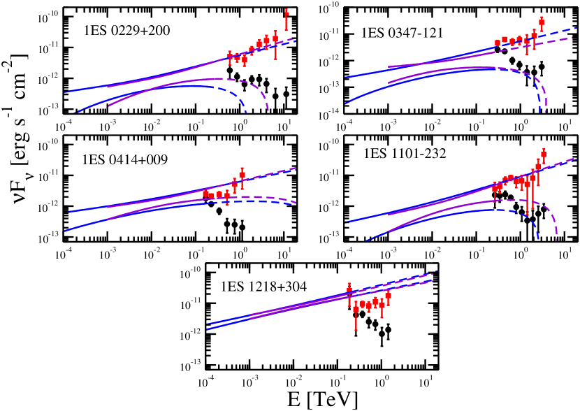
Figure 1.— The $\gamma$-ray spectra for the sources. Blue (violet) curves indicate the LAT spectra at $>0.1$ (1.0) GeV, dashed curves indicate the LAT spectra extrapolated into the VHE region. Circles indicate the observed VHE spectrum from ground-based atmospheric Cherenkov telescopes, and squares indicate the VHE spectrum deabsorbed with the EBL model of Finke et al. (2010).

3.3. Ruling out Models

Our technique for ruling out a model is illustrated in Figure 2 and has the following steps:

1. Select the model we wish to consider. This includes selecting an EBL model from the literature, selecting an IGMF strength ($B_{IG}$) and coherence length ($L_{B}$). It is also necessary to select a blazar opening angle.

2. Given the integrated 0.1–300 GeV LAT flux ($F_{LAT}$) and photon index ($\Gamma$) and their errors for a particular blazar found with the analysis discussed in Section 2, we draw a random $F_{LAT}$ and $\Gamma$ from a probability distribution function (PDF) which represents their errors. The distribution function used is discussed in Section 3.4.

3. For each energy bin of the VHE spectrum, with a measured flux and error, we draw a random flux, $F_{VHE}$, assuming the flux errors are distributed as a normal distribution (see Section 3.4). Each randomly drawn $F_{VHE}(E)$ is deabsorbed with the EBL model we are testing to give an intrinsic flux, $F_{VHE,int}(E)=\exp(\tau_{\gamma\gamma}(E))F_{VHE}(E)$.

4. From $F_{VHE,int}(E)$, the contribution of the $e^{+}e^{-}$ pairs Compton-scattering the CMB, is calculated. Two of these cascades are calculated: $F_{cascade,min}$, a cascade with the parameters $t_{\rm blazar}$ and $E_{max}$ chosen to minimize the cascade; and $F_{cascade,max}$, with the parameters chosen to maximize the cascade. These cascades are calculated in the same energy range as the LAT flux, i.e., 0.1 – 300 GeV. Here $t_{\rm blazar}$ is the length of time the blazar has been emitting $\gamma$ rays with its current luminosity (Dermer et al., 2011), and $E_{max}$ is the maximum energy of the VHE emission used to calculate the cascade. Calculating two cascade components allows us to provide more conservative constraints. The cascade flux $F_{cascade}$ is calculated using the formula of Dermer et al. (2011) and Dermer (2013). The minor corrections to this formula from Meyer et al. (2012) should have no effect on the results, since they affect the lowest flux portion of the cascade spectrum. This calculation is compared with MC cascade calculations from the literature in Appendix A.

5. The randomly drawn LAT power-law spectrum from step 2 is extrapolated to the VHE regime. For this MC iteration, the model is considered rejected if one of two criteria are met: (i) the minimum cascade flux from step 4, $F_{cascade,min}$, integrated over the LAT bandpass exceeds the randomly drawn LAT integrated flux from step 2, $F_{LAT}$; or (ii) any one of the deabsorbed flux bins from step 2, $F_{VHE,int}(E)$ exceed the extrapolated LAT flux, $F_{LAT,ext}$, unless $0.01F_{LAT}\leq F_{cascade,max}$ in which case the model is never rejected for this iteration. If the cascade flux makes up a significant fraction of the observed LAT flux, we do not believe it can be extrapolated to the VHE regime and used to constrain models, since in this case we cannot know the intrinsic spectrum in this energy range. The rejection criteria in this step are based on ones from Georganopoulos et al. (2010) and Meyer et al. (2012).

6. Steps 2–5 above are repeated $N_{\rm trials}$ times (we use $N_{\rm trials}=10^{6}$) and the number of times the model is rejected $N_{reject}$ is counted. From this, a test statistic is created: $TS=-2\ln(N_{\rm accept}/N_{\rm trials})$. Assuming the $TS$ is distributed as a $\chi^{2}$ distribution, the p-value for ruling out a model is calculated. For models ruled out by the cascade constraint, this distribution has 2 degrees of freedom; for models ruled out by the VHE points exceeding the extrapolated LAT spectrum, it has $2N_{VHE}$ degrees of freedom, where $N_{VHE}$ is the number of VHE points. That is, the significance for ruling out a model was calculated from Fisher’s method.

In Step 3, each energy bin of the VHE spectra are deabsorbed assuming the entire bin is at the central energy of the bin. Although this could conceivably introduce a systematic error, under the reasonable assumption that $\tau_{\gamma\gamma}(E)$ is not changing rapidly within each energy bin, we expect the effect to be negligible.

In Step 5, the fraction 0.01 was chosen because if the cascade spectrum contributes less than 1% to the LAT spectrum, the LAT spectrum can be safely extrapolated into the VHE range. This is an arbitrary choice, but also a very conservative one. If the cascade spectrum contributed more than 1% (say, 10%) then the LAT spectrum could still probably be safely extrapolated into the VHE regime.

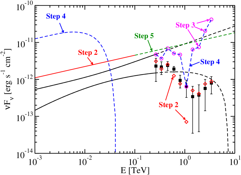
Figure 2.— This figure illustrates many of the steps in our method for ruling out models from Section 3.3, using the $\gamma$-ray spectrum for 1ES 1101-232. The LAT spectrum is shown as the bowtie, along with this spectrum extrapolated to the VHE regime as the dashed curves. The observed HESS spectrum is shown as the filled squares. The randomly drawn HESS points shown as empty diamonds ($F_{VHE}$) and the randomly drawn LAT spectrum is shown as a line, both of which are labeled “Step 2”. The deabsorbed points are shown as the circles ($F_{VHE,int}$) and labeled “Step 3”. The cascaded component and the interpolated VHE spectrum used to calculate it are shown as dashed curves labeled “Step 4”. The LAT spectrum extrapolated into the VHE regime is shown as the dashed line labeled “Step 5”. For the MC iteration shown here, the model is ruled out by both criterion in Step 5, since $F_{LAT}<F_{cascade}$ and for several points $F_{LAT,ext}<F_{VHE,int}$.

3.4. Probability Distribution Function

Many of the sources used in our sample are not very bright in the LAT, and have relatively large errors on their integrated photon flux, $F_{LAT}$. Consequently, we found that a bivariate normal probability distribution did not describe accurately the errors in $F_{LAT}$ and photon index, $\Gamma$ from the likelihood analysis to the LAT data. This PDF faced the problem that there is a significant probability that $F_{LAT}<0$, which is clearly unphysical. We plotted the PDF error points determined from the $LL$ function with several functions representing the PDF for each source spectrum; an example is seen in Figure 3. Based on these plots, we determined that a log-normal distribution was a good representation of the PDF for the $>100\ \mathrm{MeV}$ spectra, while a Gamma distribution was a good representation for the $>1\ \mathrm{GeV}$ spectra. Consequently we used a bivariate normal distribution to represent the joint PDF for the parameters from the $>100\ \mathrm{MeV}$ LAT power-law fit, $\Gamma_{LAT}$, and $w=\log_{10}(F_{LAT})$,

$$p(F_{LAT},\Gamma) =\frac{1}{2\pi\sigma_{w}\sigma_{\Gamma_{LAT}}\sqrt{1-\rho^{2}}}$$

$$\times\exp\Biggr{\{}-\frac{(w-\mu_{w})^{2}}{2(1-\rho^{2})\sigma_{w}^{2}}-\frac{(\Gamma_{LAT}-\mu_{\Gamma_{LAT}})^{2}}{2(1-\rho^{2})\sigma_{\Gamma_{LAT}}^{2}}$$

$$+\frac{\rho(w-\mu_{w})(\Gamma_{LAT}-\mu_{\Gamma_{LAT}})}{(1-\rho^{2})\sigma_{w}\sigma_{\Gamma_{LAT}}}\Biggr{\}}\$$ (1)

where $\mu_{w}$ ($\mu_{\Gamma}$) is the measured $\log_{10}(F_{LAT})$ ($\Gamma$), $\sigma_{w}$ ($\sigma_{\Gamma}$) is the standard error from the power-law fit to the LAT data for $\log_{10}(F_{LAT})$ ($\Gamma$), and $\rho$ is the correlation coefficient between $\log_{10}(F_{LAT})$ and $\Gamma$ (i.e., the covariance is $\rho\sigma_{w}\sigma_{\Gamma}$). The error in $\log_{10}(F_{LAT})$ is calculated from the error in the flux ($\sigma_{F_{LAT}}$) with $\sigma_{w}=\sigma_{F_{LAT}}/(F_{LAT}\ln(10))$.

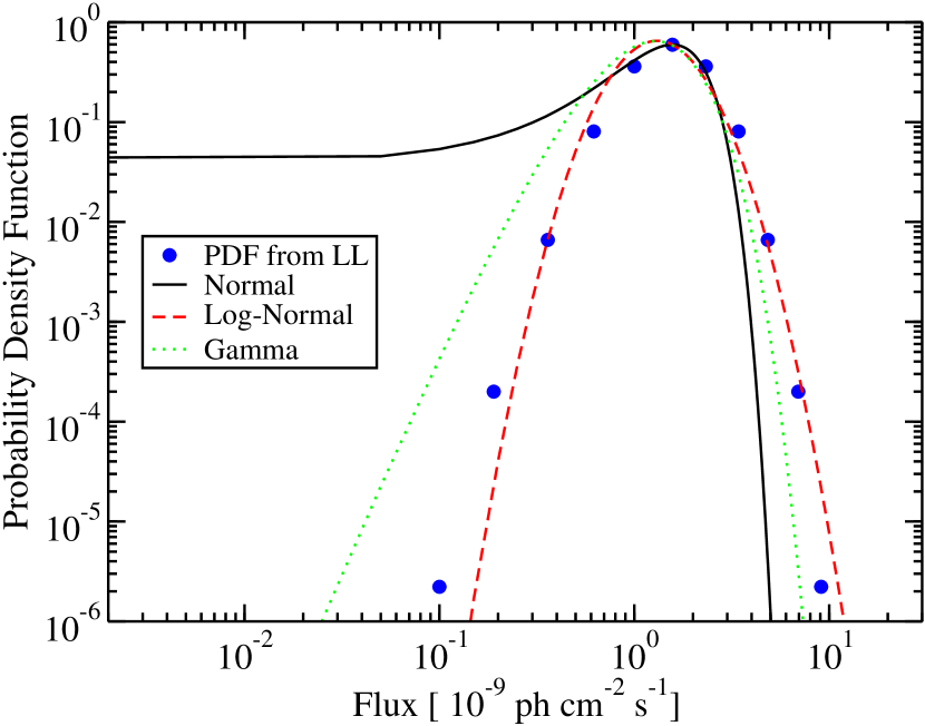
Figure 3.— The PDF for the $>100$ MeV flux for 1ES 1101$-$232 as determined from the $LL$ plotted with several functional forms of the PDF: a Normal distribution, a log-normal distribution, and a Gamma distribution.

For the $>1\ \mathrm{GeV}$ spectra, where a Gamma distribution best represented the flux from the power-law fit, we created an ad hoc bivariate probability distribution based on a Gamma distribution. It is given by

$$p(F_{LAT},\Gamma) =\frac{F_{LAT}^{\alpha_{F}-1}e^{-F_{LAT}/\beta_{F}}}{\Gamma_{f}(\alpha_{F})\beta_{F}^{\alpha_{F}}}\ \frac{1}{\sigma_{\Gamma}\sqrt{2\pi(1-\rho)}}\$$ (2)

$$\times\exp\Biggr{\{}-\frac{(\Gamma-\mu_{\Gamma})^{2}}{2(1-\rho^{2})\sigma_{\Gamma}^{2}}$$

$$+\frac{\rho(F_{LAT}-\mu_{F})(\Gamma-\mu_{\Gamma})}{(1-\rho^{2})\sigma_{F}\sigma_{\Gamma}}$$

$$-\frac{\rho^{2}(F_{LAT}-\mu_{F})^{2}}{2(1-\rho^{2})\sigma_{F}^{2}}\Biggr{\}}\ ,$$

where $\mu_{F}$ ($\mu_{\Gamma}$) is the measured $F_{LAT}$ ($\Gamma$), and $\sigma_{F}$ ($\sigma_{\Gamma}$) is the standard error from the power-law fit to the LAT data for $F_{LAT}$ ($\Gamma$), $\alpha_{F}=(\mu_{F}/\sigma_{F})^{2}$, $\beta_{F}=\sigma_{F}^{2}/\mu_{F}$, $\rho$ is the correlation coefficient between $F_{LAT}$ and $\Gamma$ (i.e., the covariance is $\rho\sigma_{F}\sigma_{\Gamma}$), and

$$\Gamma_{f}(x)=\int_{0}^{\infty}\ dy\ e^{-y}\ y^{x-1}\$$ (3)

is the standard Gamma function. This distribution was constructed to resemble a Gamma distribution for $F_{LAT}$, a normal distribution for $\Gamma$, preserve the correlated errors of a bivariate normal distribution, be normalized to unity, and reduce to a bivariate normal distribution for $\alpha_{F}\gg 1$. The latter two properties are explored in Appendix B. This bivariate PDF is not unlike the gamma-normal distribution explored by Alzaatreh et al. (2014), although their distribution does not preserve the correlation between the two variables, and so is not useful for our purposes.

The errors on the flux of each VHE bin is assumed to be described by a normal (Gaussian) distribution, given by

$$p(F_{VHE})=\frac{1}{\sigma_{F_{VHE}}\sqrt{2\pi}}\exp\left[-\frac{1}{2\sigma_{F_{VHE}}}(F_{VHE}-\mu_{F_{VHE}})^{2}\right]$$ (4)

where $F_{VHE}$ is the randomly drawn flux in that energy bin, and $\mu_{F_{VHE}}$ and $\sigma_{F_{VHE}}$ are the reported flux and measurement error, respectively.

3.5. Combined Constraints

For a given model (Step 1 in Section 3.3), we wish to combine the constraints from all of our objects (Table 1) to provide the strongest constraint possible for a given model. Since the results for different objects are entirely independent, this is done with Fisher’s method (Fisher, 1925; Mosteller & Fisher, 1948). We first created a test statistic for all the sources,

$$TS=-2\sum_{k=0}^{N_{s}}\ln(P_{\rm accept,k})$$

from the individual p-values for each source, $P_{\rm accept,k}$, where $N_{s}$ is the number of sources. Fisher’s method assures that the $TS$ is distributed as a $\chi^{2}$ distribution with $2N_{s}$ degrees of freedom. This $\chi^{2}$ distribution is integrated, giving the overall p-value of acceptance, $P_{\rm accept,com}$. We choose to present the combined results for rejecting a model as the equivalent number of sigma the model is rejected if the error were distributed as a normal distribution. That is, the number of sigma a model is rejected is $\Sigma=\sqrt{2}\ {\rm erf}^{-1}(P_{\rm accept,com})$.

4. Results

4.1. Results with Conservative Assumptions

Here we show the results for our conservative assumptions. We choose a jet opening angle of $\theta_{j}=0.1$ rad, roughly consistent with values from VLBI measurements (Jorstad et al., 2005), and the EBL model from Finke et al. (2010, their “model C”). For calculation of $F_{cascade,min}$ we use $t_{\rm blazar}=3$ years and $E_{max}$ equal to the central energy of the maximum observed bin from the IACTs. This $t_{\rm blazar}$ is the typical time between observations for the objects in our sample, and the typical time for which we know the sources are not variable. For calculation of $F_{cascade,max}$ we use $t_{\rm blazar}=1/H_{0}$, i.e., we assume the blazar has been emitting VHE $\gamma$ rays at the level currently observed for the entire age of the universe; and $E_{max}=100$ TeV. For calculation of $F_{cascade,max}$ the deabsorbed VHE points are fit with a power-law and extrapolated to 100 TeV to calculate the cascade component. The VHE spectrum is assumed to have a hard cutoff at $E_{max}$. That is, this assumes the source does not emit any $\gamma$ rays above $E_{max}$.

Our conservative results can be seen in Figure 4. One can see that high magnetic field values ($B\gtrsim 10^{-12}$ G for $L_{B}\gtrsim 1$ Mpc) are not significantly ruled out, while low values ($B\lesssim 10^{-16}$ G at $10^{-10}$ Mpc; $B\lesssim 10^{-21}$ G for $L_{B}\gtrsim 1$ Mpc) are ruled out at $\approx 7.2\sigma$. For $L_{B}\gtrsim 1$ Mpc, the allowed $B$ is essentially independent of $L_{B}$, since above this $L_{B}$ the electrons will lose most of their energy from scattering within a single coherence length. For $L_{B}\lesssim 1$ Mpc, the allowed $B$ goes as $B\propto L_{B}^{-1/2}$ due to the random change in direction of $B$, and hence the direction of the electrons’ acceleration, as they cross several coherence lengths. This overall dependence of the constraints on $B$ and $L_{B}$ has been pointed out previously by Neronov & Semikoz (2009) and Neronov & Vovk (2010). There is a strange shape in the contours at $1-10$ Mpc due to this transition region, and due to the coarseness of our grid, which is one order of magnitude in both $B$ and $L_{B}$.

Low magnetic field values are inconsistent with the data at $>5\sigma$. We consider this quite a significant constraint. Since many authors (e.g., Neronov & Vovk, 2010; Dermer et al., 2011) have ruled out low $B$ values if the cascade component is above the LAT $2\sigma$ upper limits, those authors are implicitly ruling out the $B$ values at the $2\sigma$ level. The high magnetic field values are not significantly ruled out. The most constraining sources in our sample for low $B$ values turned out to be 1ES 0229+200, 1ES 0347$-$121, and 1ES 1101$-$232, all of which individually ruled out low $B$ values at $\gtrsim 4.5\sigma$.

Our lower limits on $B$ are lower than what many previous authors have found in a similar fashion, but assuming $t_{\rm blazar}=1/H_{0}$ (e.g. Neronov & Vovk, 2010; Tavecchio et al., 2010, 2011; Dolag et al., 2011). We compute a constraint with this less conservative assumption on $t_{\rm blazar}$ below in Section 4.3 for comparison. Several authors have constrained the IGMF to be $B\gtrsim 10^{-18}$ G for $L_{B}=1$ Mpc by using a shorter $t_{\rm blazar}$ as we do (e.g., Dermer et al., 2011; Taylor et al., 2011; Vovk et al., 2012). Our lower limits are generally consistent with these authors, although slightly lower ($B>10^{-19}$ G). The minor difference could be due to the fact that we assume a sharp cutoff at high energies in the intrinsic spectrum at the maximum VHE energy bin observed from a source, while other authors extrapolate above this energy in some way, typically with an exponential form. This makes our results more conservative.

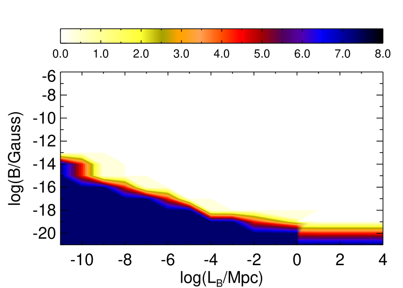
Figure 4.— The values of parameter space of $B$ and $L_{B}$ ruled out for the combined conservative results of Section 4.1 for all of our objects. The contours represent the significance a particular region of parameter space is ruled out, in number of sigma, as indicated by the bar. These constraints assume the Finke et al. (2010) EBL model and $\theta_{j}=0.1$ rad.

4.2. Robustness

In general, we consider our assumptions, and the results found in Section 4.1 quite reasonable, and indeed quite conservative. However, to be thorough, we have tested the robustness of these results by varying some of the assumptions, particularly those that would weaken the constraints, and seeing if this made a significant difference in our results.

The first item we explored is the EBL model. One would expect that the parameter space will be ruled out with greater significance if a more intense and absorbing EBL model is used, while it would be ruled out with lesser significance if a less intense EBL model is used. We performed simulations for a less intense EBL model, namely the model of Kneiske & Dole (2010). This model was designed to be as close as possible to the observed lower limits on the EBL from galaxy counts; however, note that for some regions of parameter space, other EBL models predict less absorption. The results can be seen in Figure 5. The low $B$ values are ruled out at $5.5\sigma$, while the high $B$ values are still unconstrained. We also performed simulations with the model of Franceschini et al. (2008), which has a similar overall normalization as the Finke et al. (2010) model, but its SED has a bit different shape. With this model we found that low $B$ values are ruled out at $6.7\sigma$, and high $B$ values are again unconstrained.

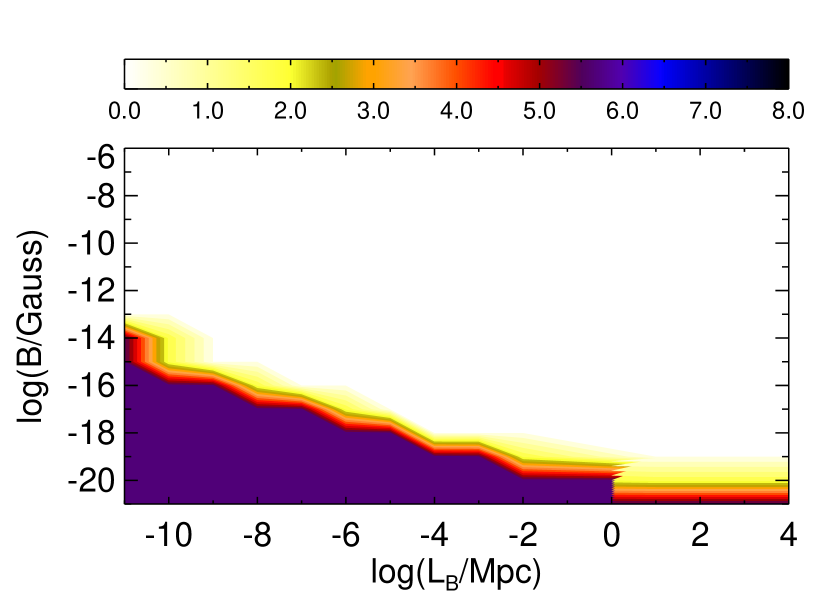
Figure 5.— The same as Figure 4, only with the EBL model of Kneiske & Dole (2010).

There is some evidence in recent years that the source 1ES 0229+200 is variable at VHE energies (Aliu et al., 2014), as is 1ES 1218+304. We have therefore computed our constraints leaving out these sources, and the results can be seen in Figure 6. Similar regions of parameter space are ruled out, but at much less significance; low values of $B$ are ruled out at $6.0\sigma$.

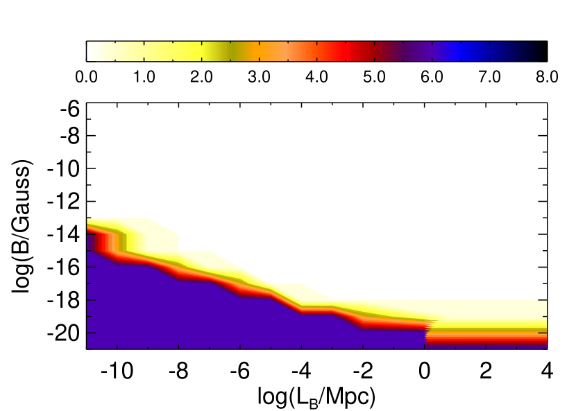
Figure 6.— The same as Figure 4, only without the results from the source 1ES 0229+200 and 1ES 1218+304, which have shown evidence for $\gamma$-ray variability.

We performed simulations with both larger ($\theta_{j}=0.2$ rad) and smaller ($\theta_{j}=0.05$ rad) values of the jet opening angle. A Larger value of $\theta_{j}$ led to larger cascades, and increased significance for ruling out the lower $B_{IG}$ values, but a decreased significance for ruling out the larger $B_{IG}$ values. Smaller values led to smaller cascades, and a decreased significance for ruling out the lower $B_{IG}$ values, and an increased significance for ruling out the larger $B_{IG}$ values. However, we found in all cases tested that the different jet opening angles made a minuscule difference, at the level of hundredths of a sigma.

We have so far used the $>0.1$ GeV LAT spectra for all sources. If we use $>1$ GeV spectra for all sources, making sure we use Equation (2) for the PDF, we find the low values of $B$ are ruled out at $6.2\sigma$.

Our method is sensitive to the highest energy points from an IACT spectrum and this could lead to a bias if such points are overestimated. Therefore, we compute our constraints throwing away the highest two VHE energy bins. In this case, the significance of ruling out the low $B$ values decreases to $5.9\sigma$.

We note that a log-normal distribution does not perfectly describe the LAT PDF for the $>100\ \mathrm{MeV}$ spectra, so we also performed our simulations with the LAT PDF described by Equation (2) rather than Equation (3.4). This increased the significance of ruling out the lower $B$ values slightly, to $7.6\sigma$.

There is some evidence of inaccuracies in the cross-calibration between the LAT and IACTs, on the order of 10–15% (Meyer et al., 2010). We performed our simulations with the VHE points scaled down by 10% and find that this decreases the significance for ruling out low $B$ values to $6.9\sigma$.

Arlen et al. (2014) use a $\chi^{2}$ fitting technique to LAT and VHE data with a primary plus cascade model with IGMF strength $B=0$, and use the quality of the fits to determine if the data are consistent with $B=0$. None of their spectra extend down to 100 MeV; thus the spectra we use that most resembles theirs is our $>1$ GeV spectra. For 1ES 0229$+$200, for two EBL models, which most resemble the model of Kneiske & Dole (2010), they found that the data are not consistent with $B=0$ at the $>2\sigma$ level. This is consistent with our results, since we found for all of our EBL models that $B>0$ at $>3.5\sigma$ for this source with $>1$ GeV spectra. Arlen et al. (2014) also do a fit with an EBL model with intensity less than 2 nW m^-2 s^-1 in the 10-20 $\mu$m range (their “EBL model 3”) and find their data are consistent with $B=0$ at the $2\sigma$ level. This EBL model is below all of the EBL models explored here, and indeed it is inconsistent with 15 $\mu$m galaxy count lower limit from Infrared Space Observatory observations (Metcalfe et al., 2003). For 1ES 0347$-$121, and 1101$-$232, Arlen et al. (2014) find that they cannot rule out $B=0$ at $>2\sigma$ with their technique. With our technique, for the Kneiske & Dole (2010) EBL model and using $>1$ GeV LAT spectra, we are also not able to rule out these sources at $>2\sigma$, so that these results are also consistent with those of Arlen et al. (2014). Combining the constraints for all sources with the Kneiske & Dole (2010) EBL model and the $>1$ GeV LAT spectra, lower $B$ values (including naturally $B=0$) are ruled out at only $2.6\sigma$. This is greater than the $2\sigma$ criterion of Arlen et al. (2014), but a much lower significance than the $>5\sigma$ constraints from our other assumptions. We also found that using the EBL model of Franceschini et al. (2008), low $B$ field values were ruled out at $4.8\sigma$ combining the results of all of our sources. Ruling out low $B$ field values at $>5\sigma$ significance depends on using $>100$ MeV spectra and the EBL model used.

4.3. Results with Less Conservative Assumptions

We have also computed constraints with less conservative assumptions. We did this by modifying step 4 in our procedure (Section 3) as follows: we used $F_{cascade,min}=F_{cascade,max}$, where both were calculated assuming $t_{\rm blazar}=1/H_{0}$ and using the maximum observed VHE photon bin for $E_{max}$. These less conservative constraints are computed here primarily for comparison with other authors, who have used similar assumptions to constrain the IGMF (e.g. Neronov & Vovk, 2010; Tavecchio et al., 2010, 2011; Dolag et al., 2011).

The less conservative constraints can be seen in Figure 7. The constraints are similar to the conservative constraints (Figure 4), with similar significance of rejection; however, a much greater region of parameter space is ruled out. In particular, $B$ is constrained to be 2-3 orders of magnitude higher than the conservative constraint. Indeed, for a given value of $L_{B}$, $B$ is constrained to within two orders of magnitude. For instance, for $L_{B}=1$ Mpc, the magnetic field strength is constrained to $B\gtrsim 10^{-16}$ G at $7.1\sigma$. In general, the lower limit is roughly consistent although still lower than what previous authors have found, who generally constrain $B\gtrsim 10^{-15}$ G at $L_{B}=1$ Mpc (Tavecchio et al., 2010; Dolag et al., 2011) although Neronov & Vovk (2010) found a lower limit of $B=3\times 10^{-16}$ G at $L_{B}\gtrsim 1$ Mpc. The reasons for this minor disagreement are probably the same as those discussed in Section 4.1.

Essey et al. (2011a) have computed both upper and lower constraints on the IGMF assuming $\gamma$ rays originate from the blazar, or alternatively, from UHECRs originating from the blazar interacting with the EBL and CMB. Only their results for the assumption of $\gamma$ rays directly from the source are directly comparable to ours, since we also make this assumption. They find constraints for various spectral indices of the intrinsic spectrum. Their lower limits on $B$ were computed in a similar fashion to other authors (e.g., Neronov & Vovk, 2010; Tavecchio et al., 2010) using the LAT upper limits and assuming the cascade emission could not exceed this. They also calculated upper limits on $B$, because they found that the cascade flux was necessary to explain the lower energy emission observed by the IACTs. For a low EBL model and a high energy cutoff in the intrinsic spectrum at 20 TeV, they find that essentially no value of $B$ is allowed for $L_{B}=1$ Mpc. For higher EBL models and higher energy cutoffs, they did find values of $B$ that were allowed, generally $B\gtrsim 10^{-16}$ G, and upper limits strongly dependent on the assumed intrinsic spectral index. Our constraints are considerably weaker, and indeed, more conservative. The main reason seems to be that we cut off the VHE spectrum at the highest observed energy bin, rather than assuming it extends to 20-100 TeV. This means the cascade flux will be lower, and it will not extend into the VHE range. Thus the criterion Essey et al. (2011a) used to obtain upper limits on $B$ are not applicable here.

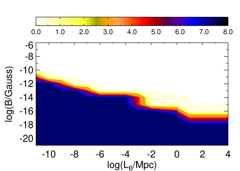
Figure 7.— The same as Figure 4, only with less conservative assumptions. Here $F_{cascade,min}=F_{cascade,max}$, and the cascade was calculated assuming $t_{\rm blazar}=1/H_{0}$ and $E_{max}$ is the maximum observed VHE photon bin from the source.

5. Discussion

We have used a combination of up-to-date Fermi-LAT observations and archival VHE IACT observations of 5 BL Lac objects to constrain the IGMF parameters $B$ and $\lambda_{B}$. These constraints rely on the assumptions outlined in Section 3.1. Our results indicate that magnetic field strength values $B\lesssim 10^{-19}$ G for $L_{B}\geq 1$ Mpc are ruled out at $>5\sigma$, with higher $B$ values ruled out for lower values of $L_{B}$, for example, if $L_{B}\approx 10^{-8}$ Mpc, $B\lesssim 10^{-15}$ G. These results are robust with respect to the choice of EBL model, VHE variability of the sources, jet opening angle, or data selection, i.e., whether $>100$ MeV or $>1$ GeV LAT spectra are used, and whether or not the highest two VHE energy bins are used. The only exceptions are using the $>1\ \mathrm{GeV}$ spectra with the EBL models of Kneiske & Dole (2010) and Franceschini et al. (2008). Using the former EBL model, low $B$ values are ruled out at $2.6\sigma$, and using the latter EBL model they are ruled out at $4.8\sigma$. We were not able to constrain high values of the IGMF, despite our efforts with a new method for doing so. We used several novel techniques in our analysis, including a MC scheme and new bivariate probability distribution to describe the errors in the LAT power-law fit. In a preliminary analysis using 42 months of data, we (Finke, Reyes, & Georganopoulos, 2013) found that large values of $B$ were ruled out at $>5\sigma$ using 1ES 0229+200 and 1ES 1101$-$232. We were unable to verify this with more data and our updated analysis (more nearby point sources, exclusion of the Sun and Moon see Section 2) and updated method for ruling out models (Section 3.3).

These results have several possible interpretations. The most straightforward is to take the constraints in Figure 4 at face value. In this interpretation, low magnetic field values are highly unlikely, at the $>5\sigma$ level, while high magnetic field values are unconstrained. In all cases, the VHE spectra are consistent with the extrapolated LAT spectra. If all our assumptions are correct, and the constraints can be taken at face value, our results have implications for the formation of the IGMF and the era of inflation. A non-helical IGMF generated from an electroweak phase transition in the radiation dominated era is essentially ruled out (Neronov & Semikoz, 2009; Wagstaff & Banerjee, 2014). The BICEP2 collaboration has claimed the detection of inflation-originating gravitational waves in the CMB polarization (Ade et al., 2014). If the IGMF originates from inflationary magnetogenesis, there is some tension between the BICEP2 result and constraints for $B\gtrsim 10^{-15}$ G (Fujita & Mukohyama, 2012; Fujita & Yokoyama, 2014; Ferreira et al., 2014). However, a joint analysis by the Planck and BICEP2/Keck Array Collaborations (Ade et al., 2015) found that the original BICEP2 analysis did not properly take into account a dust contribution to the observed polarization, so that the claimed detection of gravitational waves was in error.

We do not find any evidence for a contribution from cascade emission to the LAT flux of our sources. Thus, another possible interpretation is that plasma beam instabilities eliminate the cascade (Broderick et al., 2012, see assumption #4 in Section 3.1). See Venters & Pavlidou (2013); Miniati & Elyiv (2013); and Sironi & Giannios (2014) for critical assessments of the application of plasma beam instabilities to VHE blazars. Chang et al. (2012) argue that blazars’ VHE emission is absorbed by EBL interactions, and the resulting pairs interacting via this plasma beam instability contribute to the heating of the intergalactic medium. This in turn would prevent the formation of dwarf galaxies at late times ($z\lesssim 2$), possibly reconciling the sparsity of dwarf galaxies with respect to predictions of $\Lambda$CDM cosmology (Pfrommer et al., 2012).

We assume the LAT and VHE $\gamma$ rays are produced co-spatially in the jet of the BL Lac object (Assumption #1). However, it is possible that UHECRs produced by the object escape into intergalactic space, where they produce the VHE $\gamma$ rays observed with IACTs (Essey & Kusenko, 2010; Essey et al., 2010, 2011b). If this is the case, our results will not be valid, although it is still possible to constrain the IGMF (Essey et al., 2011a). Since a UHECR origin for VHE $\gamma$ rays would not predict any variability, if the objects used here were to be observed in the future with an IACT to be at a flux level much lower than measured previously, this would be strong evidence for the co-spatially of the LAT and IACT-detected $\gamma$ rays.

If axion-like particles existed with the relevant parameters, the VHE $\gamma$ rays could avoid EBL attenuation (assumption #3; de Angelis et al., 2007; Sánchez-Conde et al., 2009; Horns et al., 2012; Reesman & Walker, 2014; Meyer et al., 2014). This would allow VHE photons to avoid much of the $\gamma$-ray attenuation, meaning our de-absorbed VHE spectra would not be correct, and the cascade component would be lower. This would mean our $B$ constraints are not valid. If we had significantly ruled out high magnetic field values, this could have been interpreted as evidence for this mechanism for avoiding $\gamma$-ray attenuation.

The assumption that all of the cascade flux is produced inside the PSF (assumption #6) should not affect our low $B$ constraints, since the extended halos should only be observable for higher $B$ values (Neronov & Semikoz, 2009). It is possible that the reason we cannot constrain the highest $B$ values is that the cascade emission is not present because it is outside the PSF.

Therefore, one of the most straightforward ways to confirm our results would be the detection of resolved $\gamma$-ray halos by LAT or the future Cherenkov Telescope Array (CTA). These halos are expected to be resolved by the LAT if $10^{-16}\lesssim B\lesssim 10^{-14}$ G for $L_{B}\geq 1$ Mpc, and at higher values of $B$ for lower $L_{B}$ (Neronov & Semikoz, 2009). We note that both our conservative (Figure 4) and non-conservative (Figure 7) constraints allow for this region of parameter space. The detection of these halos would essentially imply that all of our assumptions (Section 3.1) are correct, except possibly assumption #1. It is possible that UHECR interactions with the EBL and CMB could also produce these $\gamma$-ray halos. The IGMF could also be constrained by observations of anisotropy in the extragalactic $\gamma$-ray background (Venters & Pavlidou, 2013). Tashiro et al. (2014) and Chen et al. (2015) find a preference for photons of decreasing energy in the LAT extragalactic $\gamma$-ray background to be preferentially bent to the left. They interpret this as evidence for a helical IGMF with $B\sim 10^{-14}\ \mathrm{G}$ and $L_{B}\sim 10$ Mpc, which would be consistent with our results.

Appendix A Comparison of Cascade Calculation with Calculations from the Literature

We have made use of the simple analytic cascade calculation described by Dermer et al. (2011) and Dermer (2013). This calculation has the advantage of being relatively quick to calculate numerically. In this appendix, we compare it to more extensive MC cascade calculations from the literature, those from Taylor et al. (2011), Kachelrieß et al. (2012), and Arlen et al. (2014). We will use cascades calculated for 1ES 0229+200, a common source used for these sorts of constraints. The primary $\nu F_{\nu}$ spectrum from the source in all cases can be parameterized as

$$F(E)=F_{0}\left(\frac{E}{E_{0}}\right)^{2-\Gamma}e^{-E/E_{cut}}\$$ (A1)

with free parameters $F_{0}$, $\Gamma$, and $E_{cut}$. We choose to normalize the primary spectrum at $E_{0}=1$ TeV.

Table 2Parameters for cascade calculation in figures. Parameters that are varied within each figure are labeled as “v”.

Parameter	Fig. 8	Fig. 9	Fig. 10	Fig. 11
$\Gamma$	1.2	1.2	0.67	1.3
$E_{cut}$ [TeV]	5.0	5.0	20	1
$F_{0}$ [$10^{-12}\ \mathrm{erg}\ \mathrm{cm}^{-2}\ \mathrm{s}^{-1}$]	$4.6$	4.6	1.1	12
$B_{IG}$ [G]	v	v	$10^{-17}$	0.0
$L_{B}$ [Mpc]	1.0	1.0	1.0	1.0
$t_{blazar}$ [yr]	$H_{0}^{-1}$	3	v	$H_{0}^{-1}$
EBL model	KD10	KD10	F08	F10

In Figures 8 and 9 we attempt to reproduce several of the results of Taylor et al. (2011) with our simple cascade calculation. Figure 8 can be compared with the first panel of Figure 7 of Taylor et al. (2011). This calculation assumes that the blazar has been producing the primary $\gamma$-ray spectrum for the age of the universe. The cascade results appear to be in very good agreement. In Figure 9 we perform a calculation with parameters similar to the second panel of Figure 7 from Taylor et al. (2011), where the blazar has been producing VHE $\gamma$ rays for 3 years. In this case, the agreement is less good. In general, our calculation predicts lower emission at the lower energies than the MC of Taylor et al. (2011). We conclude that our results are thus very conservative, since they under-predict the cascade from more detailed calculations.

In Figure 10 we produce a cascade calculation with the same parameters as those from the right panel of Figure 3 of Kachelrieß et al. (2012). Again, our calculation under-predicts the lower energy emission compared to their detailed calculations, which implies that our results are very conservative.

In Figure 11 we reproduce Figure 9 from Arlen et al. (2014), who test $B=0$. Our cascade calculation is similar to theirs, but a bit lower by a factor of $\approx 1.4$.

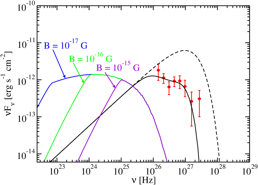
Figure 8.— The cascade spectrum of 1ES 0229+200, calculated with parameters similar to those of the calculation shown in Fig. 7, first panel of Taylor et al. (2011). The HESS spectrum (Aharonian et al., 2007d) is shown as the diamonds, the primary, unabsorbed spectrum is shown as the dashed line, and the primary absorbed spectrum as the solid line going through the HESS data points. The cascade spectra are labeled by the IGMF strength used in the calculation. Other parameters are shown in Table 2.

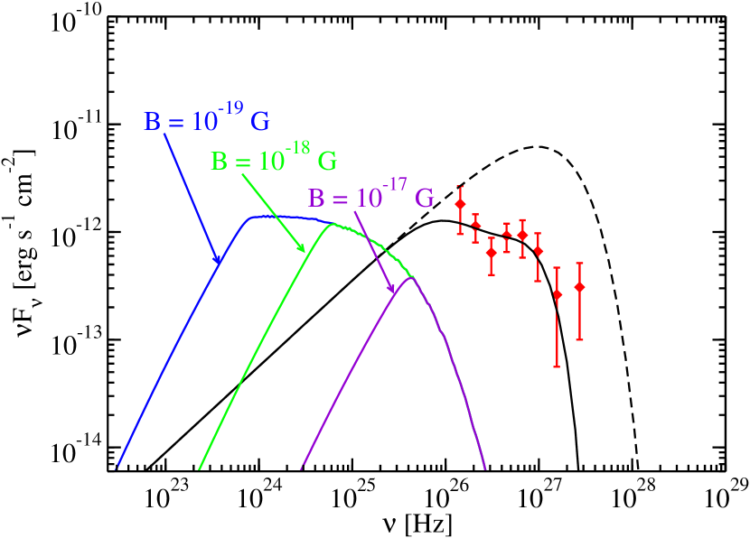
Figure 9.— The cascade spectrum of 1ES 0229+200, calculated with parameters similar to those of the calculation shown in Fig. 7, second panel of Taylor et al. (2011). The HESS spectrum (Aharonian et al., 2007d) is shown as the diamonds, the primary, unabsorbed spectrum is shown as the dashed line, and the primary absorbed spectrum as the solid line going through the HESS data points. The cascade spectra are labeled by the IGMF strength used in the calculation. Other parameters are shown in Table 2.

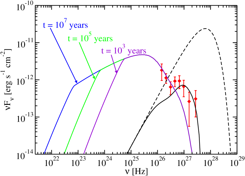
Figure 10.— The cascade spectrum of 1ES 0229+200, calculated with parameters similar to those of the calculation shown in the right panel of Fig. 3 of Kachelrieß et al. (2012). The HESS spectrum (Aharonian et al., 2007d) is shown as the diamonds, the primary, unabsorbed spectrum is shown as the dashed line, and the primary absorbed spectrum as the solid line going through the HESS data points. The cascade spectra are labeled by the jet time used in the calculation. Other parameters are shown in Table 2.

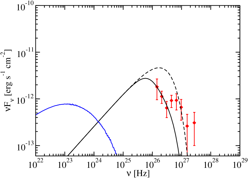
Figure 11.— The cascade spectrum of 1ES 0229+200, calculated with parameters similar to those of the calculation shown in the right panel of Fig. 9 of Arlen et al. (2014). The HESS spectrum (Aharonian et al., 2007d) is shown as the diamonds, the primary, unabsorbed spectrum is shown as the dashed line, and the primary absorbed spectrum as the solid line going through the HESS data points. The cascade spectra are labeled by the jet time used in the calculation. Other parameters are shown in Table 2.

Appendix B Properties of PDF

In this appendix, we explore two properties of the PDF given by Equation (2),

$$p(x,y) =\frac{x^{\alpha_{x}-1}e^{-x/\beta_{x}}}{\Gamma_{f}(\alpha_{x})\beta_{x}^{\alpha_{x}}}\ \frac{1}{\sigma_{y}\sqrt{2\pi(1-\rho)}}\$$ (B1)

$$\times\exp\left\{-\frac{(y-\mu_{y})^{2}}{2(1-\rho^{2})\sigma_{y}^{2}}+\frac{\rho(x-\mu_{x})(y-\mu_{y})}{(1-\rho^{2})\sigma_{x}\sigma_{y}}-\frac{\rho^{2}(x-\mu_{x})^{2}}{2(1-\rho^{2})\sigma_{x}^{2}}\right\}\ ,$$

where the notation has been simplified by letting $F_{LAT}\rightarrow x$ and $\Gamma\rightarrow y$.

First we show that Equation (B1) reduces to a bivariate normal distribution for $\alpha_{x}=(\mu_{x}/\sigma_{x})^{2}\gg 1$ and $x$ is close to $\mu_{x}$. We begin by making use of the Sterling Approximation,

$$\Gamma(\alpha)\approx\sqrt{\frac{2\pi}{\alpha}}\left(\frac{\alpha}{e}\right)^{\alpha},\;\;\alpha\gg 1$$ (B2)

which leads to

$$p(x,y) =\frac{1}{2\pi\sigma_{x}\sigma_{y}\sqrt{1-\rho^{2}}}\left(\frac{x}{\mu_{x}}\right)^{\alpha_{x}-1}\exp\left\{\frac{\mu_{x}^{2}-x\mu_{x}}{\sigma_{x}^{2}}\right\}\$$

$$\times\exp\left\{-\frac{(y-\mu_{y})^{2}}{2(1-\rho^{2})\sigma_{y}^{2}}+\frac{\rho(x-\mu_{x})(y-\mu_{y})}{(1-\rho^{2})\sigma_{x}\sigma_{y}}-\frac{\rho^{2}(x-\mu_{x})^{2}}{2(1-\rho^{2})\sigma_{x}^{2}}\right\}\ .$$ (B3)

The Taylor expansion of the natural logarithm is

$$\ln(1+x)=x-\frac{x^{2}}{2}+\frac{x^{3}}{3}-\ldots$$ (B4)

which can be rewritten

$$\left(1+\frac{x}{a}\right)^{a}=\exp\left\{x-\frac{x^{2}}{2a}+\frac{x^{3}}{3a^{2}}-\ldots\right\}$$ (B5)

for $x/a\ll 1$. Using this one can show, with some algebraic manipulation, that

$$\left(\frac{x}{\mu_{x}}\right)^{\alpha_{x}-1} \approx\left(\frac{x}{\mu_{x}}\right)^{\alpha_{x}}=\left(1-1+\frac{x}{\mu_{x}}\right)^{\alpha_{x}}$$

$$\approx\left(1+\frac{(x-\mu_{x})\alpha_{x}}{\mu_{x}\alpha_{x}}\right)^{\alpha_{x}}=\left(1+\frac{(x-\mu_{x})\mu_{x}}{\sigma_{x}^{2}\alpha_{x}}\right)^{\alpha_{x}}$$

$$\approx\exp\left\{\frac{(x-\mu_{x})\mu_{x}}{\sigma_{x}^{2}}-\frac{(x-\mu_{x})^{2}\mu_{x}^{2}}{2\sigma_{x}^{4}\alpha_{x}}+\ldots\right\}$$

$$\approx\exp\left\{\frac{x\mu_{x}-\mu_{x}^{2}}{\sigma_{x}^{2}}-\frac{(x-\mu_{x})^{2}}{2\sigma_{x}^{2}}\right\}\ .$$ (B6)

Substitution of this into Equation (B) results in

$$p(x,y) \approx\frac{1}{2\pi\sigma_{x}\sigma_{y}\sqrt{1-\rho^{2}}}$$

$$\times\exp\left\{-\frac{(x-\mu_{x})^{2}}{2(1-\rho^{2})\sigma_{x}^{2}}-\frac{(y-\mu_{y})^{2}}{2(1-\rho^{2})\sigma_{y}^{2}}+\frac{\rho(x-\mu_{x})(y-\mu_{y})}{(1-\rho^{2})\sigma_{x}\sigma_{y}}\right\}\$$ (B7)

which is the bivariate normal distribution.

Next, we show that the PDF, Equation (B1) is normalized to unity. That is,

$$1=\int_{-\infty}^{\infty}\int_{0}^{\infty}\ dy\ dx\ p(x,y)\equiv J\ .$$ (B8)

We begin by performing the integral over $y$,

$$J_{y}=\int_{-\infty}^{\infty}\ dy\ \exp\left\{\frac{-(y-\mu_{y})^{2}}{2(1-\rho^{2})\sigma_{y}^{2}}+\frac{\rho(x-\mu_{x})(y-\mu_{y})}{(1-\rho^{2})\sigma_{x}\sigma_{y}}\right\}\ .$$ (B9)

We make the substitution

$$\frac{(y-\mu_{y})^{2}}{2(1-\rho^{2})\sigma_{y}^{2}}=u^{2},$$ (B10)

giving $dy=\left[2(1-\rho^{2})\right]^{1/2}\sigma_{y}\ du$ and

$$J_{y}=\sigma_{y}\left[2(1-\rho^{2})\right]^{1/2}\int_{-\infty}^{\infty}\ du\ \exp\left\{-u^{2}+u\ \frac{\rho(x-\mu_{x})}{\sigma_{x}}\sqrt{\frac{2}{1-\rho^{2}}}\right\}\ .$$ (B11)

This integral is tabulated, and the result is

$$J_{y}=\sigma_{y}\left[2\pi(1-\rho^{2})\right]^{1/2}\exp\left\{\frac{\rho^{2}(x-\mu_{x})^{2}}{2\sigma_{x}^{2}(1-\rho^{2})}\right\}\ .$$ (B12)

Next we must do the integral over $x$. Putting this result into Equation (B8) gives

$$J=\frac{1}{\Gamma_{f}(\alpha_{x})\beta_{x}^{\alpha_{x}}}\int_{-\infty}^{\infty}\ dx\ x^{\alpha_{x}-1}\ e^{-x/\beta_{x}}$$ (B13)

which is the integral of the Gamma distribution. It is well-known to be normalized to unity.

References

- Abdo et al. (2009) Abdo, A. A., et al. 2009, ApJ, 707, 1310
- Abdo et al. (2010) —. 2010, ApJ, 723, 1082
- Abramowski et al. (2012) Abramowski, A., et al. 2012, A&A, 538, A103
- Abramowski et al. (2013) —. 2013, A&A, 550, A4
- Acciari et al. (2009) Acciari, V. A., et al. 2009, ApJ, 695, 1370
- Acciari et al. (2010) —. 2010, ApJ, 708, L100
- Acero et al. (2015) Acero, F., et al. 2015, ApJS, 218, 23
- Ackermann et al. (2012) Ackermann, M., et al. 2012, Science, 338, 1190
- Ackermann et al. (2013) —. 2013, ApJ, 765, 54
- Ackermann et al. (2015) —. 2015, ApJS, submitted, arXiv:1501.06054
- Ade et al. (2015) Ade, P. A. R., Aghanim, N., Ahmed, Z., Aikin, R. W., Alexander, K. D., Arnaud, M., Aumont, J., & et al. 2015, arXiv:1502.00612
- Ade et al. (2014) Ade, P. A. R., et al. 2014, Physical Review Letters, 112, 241101
- Aharonian et al. (2006) Aharonian, F., et al. 2006, Nature, 440, 1018
- Aharonian et al. (2007a) —. 2007a, ApJ, 664, L71
- Aharonian et al. (2007b) —. 2007b, A&A, 470, 475
- Aharonian et al. (2007c) —. 2007c, A&A, 473, L25
- Aharonian et al. (2007d) —. 2007d, A&A, 475, L9
- Aharonian et al. (1994) Aharonian, F. A., Coppi, P. S., & Voelk, H. J. 1994, ApJ, 423, L5
- Aharonian et al. (2008) Aharonian, F. A., Khangulyan, D., & Costamante, L. 2008, MNRAS, 387, 1206
- Aharonian et al. (2002) Aharonian, F. A., Timokhin, A. N., & Plyasheshnikov, A. V. 2002, A&A, 384, 834
- Aharonian et al. (1999) Aharonian, F. A., et al. 1999, A&A, 349, 11
- Albert et al. (2008) Albert, J., et al. 2008, Science, 320, 1752
- Aliu et al. (2014) Aliu, E., et al. 2014, ApJ, 782, 13
- Alzaatreh et al. (2014) Alzaatreh, A., Famoye, F., & Lee, C. 2014, Comput. Stat. Data Anal., 69, 67
- Ando & Kusenko (2010) Ando, S., & Kusenko, A. 2010, ApJ, 722, L39
- Arlen et al. (2014) Arlen, T. C., Vassilev, V. V., Weisgarber, T., Wakely, S. P., & Yusef Shafi, S. 2014, ApJ, 796, 18
- Atwood et al. (2009) Atwood, W. B., et al. 2009, ApJ, 697, 1071
- Bernstein (2007) Bernstein, R. A. 2007, ApJ, 666, 663
- Bernstein et al. (2002) Bernstein, R. A., Freedman, W. L., & Madore, B. F. 2002, ApJ, 571, 56
- Biller et al. (1995) Biller, S. D., et al. 1995, ApJ, 445, 227
- Böttcher et al. (2008) Böttcher, M., Dermer, C. D., & Finke, J. D. 2008, ApJ, 679, L9
- Broderick et al. (2012) Broderick, A. E., Chang, P., & Pfrommer, C. 2012, ApJ, 752, 22
- Chang et al. (2012) Chang, P., Broderick, A. E., & Pfrommer, C. 2012, ApJ, 752, 23
- Chang et al. (2014) Chang, P., Broderick, A. E., Pfrommer, C., Puchwein, E., Lamberts, A., & Shalaby, M. 2014, ApJ, 797, 110
- Chen et al. (2004) Chen, A., Reyes, L. C., & Ritz, S. 2004, ApJ, 608, 686
- Chen et al. (2015) Chen, W., Chowdhury, B. D., Ferrer, F., Tashiro, H., & Vachaspati, T. 2015, MNRAS, 450, 3371
- Costamante (2013) Costamante, L. 2013, International Journal of Modern Physics D, 22, 30025
- Dai et al. (2002) Dai, Z. G., Zhang, B., Gou, L. J., Mészáros, P., & Waxman, E. 2002, ApJ, 580, L7
- de Angelis et al. (2007) de Angelis, A., Roncadelli, M., & Mansutti, O. 2007, Phys. Rev. D, 76, 121301
- Dermer (2013) Dermer, C. D. 2013, in Astrophysics at Very High Energies, Saas-Fee Advanced Course, Volume 40. ISBN 978-3-642-36133-3. Springer-Verlag Berlin Heidelberg, 2013, p. 225, ed. F. Aharonian, L. Bergström, & C. Dermer, 225
- Dermer et al. (2011) Dermer, C. D., Cavadini, M., Razzaque, S., Finke, J. D., Chiang, J., & Lott, B. 2011, ApJ, 733, L21
- Dolag et al. (2011) Dolag, K., Kachelriess, M., Ostapchenko, S., & Tomàs, R. 2011, ApJ, 727, L4
- Domínguez et al. (2013) Domínguez, A., Finke, J. D., Prada, F., Primack, J. R., Kitaura, F. S., Siana, B., & Paneque, D. 2013, ApJ, 770, 77
- Domínguez et al. (2011) Domínguez, A., et al. 2011, MNRAS, 410, 2556
- Dwek & Krennrich (2013) Dwek, E., & Krennrich, F. 2013, Astroparticle Physics, 43, 112
- Dwek & Slavin (1994) Dwek, E., & Slavin, J. 1994, ApJ, 436, 696
- Dwek et al. (1998) Dwek, E., et al. 1998, ApJ, 508, 106
- Edelstein et al. (2000) Edelstein, J., Bowyer, S., & Lampton, M. 2000, ApJ, 539, 187
- Essey et al. (2011a) Essey, W., Ando, S., & Kusenko, A. 2011a, Astroparticle Physics, 35, 135
- Essey et al. (2011b) Essey, W., Kalashev, O., Kusenko, A., & Beacom, J. F. 2011b, ApJ, 731, 51
- Essey et al. (2010) Essey, W., Kalashev, O. E., Kusenko, A., & Beacom, J. F. 2010, Physical Review Letters, 104, 141102
- Essey & Kusenko (2010) Essey, W., & Kusenko, A. 2010, Astroparticle Physics, 33, 81
- Fazio & Stecker (1970) Fazio, G. G., & Stecker, F. W. 1970, Nature, 226, 135
- Ferreira et al. (2014) Ferreira, R. J. Z., Jain, R. K., & Sloth, M. S. 2014, J. Cosmology Astropart. Phys, 6, 53
- Finke et al. (2013) Finke, J., Reyes, L., & Georganopoulos, M. 2013, arXiv:1303.5093
- Finke & Razzaque (2009) Finke, J. D., & Razzaque, S. 2009, ApJ, 698, 1761
- Finke et al. (2010) Finke, J. D., Razzaque, S., & Dermer, C. D. 2010, ApJ, 712, 238
- Fisher (1925) Fisher, R. A. 1925, Statistical Methods for Research Workers (Edinburgh: Oliver & Boyd)
- Franceschini et al. (2008) Franceschini, A., Rodighiero, G., & Vaccari, M. 2008, A&A, 487, 837
- Fujita & Mukohyama (2012) Fujita, T., & Mukohyama, S. 2012, J. Cosmology Astropart. Phys, 10, 34
- Fujita & Yokoyama (2014) Fujita, T., & Yokoyama, S. 2014, J. Cosmology Astropart. Phys, 3, 13
- Furniss et al. (2013) Furniss, A., et al. 2013, ApJ, 768, L31
- Georganopoulos et al. (2010) Georganopoulos, M., Finke, J. D., & Reyes, L. C. 2010, ApJ, 714, L157
- Georganopoulos et al. (2008) Georganopoulos, M., Sambruna, R. M., Kazanas, D., Cillis, A. N., Cheung, C. C., Perlman, E. S., Blundell, K. M., & Davis, D. S. 2008, ApJ, 686, L5
- Gilmore (2012) Gilmore, R. C. 2012, MNRAS, 420, 800
- Gilmore et al. (2009) Gilmore, R. C., Madau, P., Primack, J. R., Somerville, R. S., & Haardt, F. 2009, MNRAS, 399, 1694
- Gilmore et al. (2012) Gilmore, R. C., Somerville, R. S., Primack, J. R., & Domínguez, A. 2012, MNRAS, 422, 3189
- Gould & Schréder (1967) Gould, R. J., & Schréder, G. P. 1967, Physical Review, 155, 1408
- Hartman et al. (1992) Hartman, R. C., et al. 1992, ApJ, 385, L1
- Hauser & Dwek (2001) Hauser, M. G., & Dwek, E. 2001, ARA&A, 39, 249
- Hauser et al. (1998) Hauser, M. G., et al. 1998, ApJ, 508, 25
- Horns et al. (2012) Horns, D., Maccione, L., Meyer, M., Mirizzi, A., Montanino, D., & Roncadelli, M. 2012, Phys. Rev. D, 86, 075024
- Ichiki et al. (2008) Ichiki, K., Inoue, S., & Takahashi, K. 2008, ApJ, 682, 127
- Johannesson et al. (2013) Johannesson, G., Orlando, E., & for the Fermi-LAT collaboration. 2013, arXiv:1307.0197
- Jorstad et al. (2005) Jorstad, S. G., et al. 2005, AJ, 130, 1418
- Kachelrieß et al. (2012) Kachelrieß, M., Ostapchenko, S., & Tomàs, R. 2012, Computer Physics Communications, 183, 1036
- Kneiske & Dole (2010) Kneiske, T. M., & Dole, H. 2010, A&A, 515, A19
- Lefa et al. (2011) Lefa, E., Aharonian, F. A., & Rieger, F. M. 2011, ApJ, 743, L19
- Leinert et al. (1998) Leinert, C., et al. 1998, A&AS, 127, 1
- Madau & Phinney (1996) Madau, P., & Phinney, E. S. 1996, ApJ, 456, 124
- Madau & Pozzetti (2000) Madau, P., & Pozzetti, L. 2000, MNRAS, 312, L9
- Mankuzhiyil et al. (2011) Mankuzhiyil, N., Ansoldi, S., Persic, M., & Tavecchio, F. 2011, ApJ, 733, 14
- Marsden et al. (2009) Marsden, G., et al. 2009, ApJ, 707, 1729
- Matsuoka et al. (2011) Matsuoka, Y., Ienaka, N., Kawara, K., & Oyabu, S. 2011, ApJ, 736, 119
- Mattila (2003) Mattila, K. 2003, ApJ, 591, 119
- Mattox et al. (1996) Mattox, J. R., et al. 1996, ApJ, 461, 396
- Maurer et al. (2012) Maurer, A., Raue, M., Kneiske, T., Horns, D., Elsässer, D., & Hauschildt, P. H. 2012, ApJ, 745, 166
- Mazin & Raue (2007) Mazin, D., & Raue, M. 2007, A&A, 471, 439
- Menzler & Schlickeiser (2015) Menzler, U., & Schlickeiser, R. 2015, MNRAS, 448, 3405
- Metcalfe et al. (2003) Metcalfe, L., et al. 2003, A&A, 407, 791
- Meyer et al. (2010) Meyer, M., Horns, D., & Zechlin, H.-S. 2010, A&A, 523, A2
- Meyer et al. (2014) Meyer, M., Montanino, D., & Conrad, J. 2014, J. Cosmology Astropart. Phys, 9, 3
- Meyer et al. (2012) Meyer, M., Raue, M., Mazin, D., & Horns, D. 2012, A&A, 542, A59
- Miniati & Elyiv (2013) Miniati, F., & Elyiv, A. 2013, ApJ, 770, 54
- Mohanty et al. (1993) Mohanty, G., et al. 1993, in International Cosmic Ray Conference, Vol. 1, International Cosmic Ray Conference, 440
- Mosteller & Fisher (1948) Mosteller, F., & Fisher, R. A. 1948, American Statistician, 2, 30
- Murase et al. (2008) Murase, K., Takahashi, K., Inoue, S., Ichiki, K., & Nagataki, S. 2008, ApJ, 686, L67
- Murthy et al. (2001) Murthy, J., Henry, R. C., Shelton, R. L., & Holberg, J. B. 2001, ApJ, 557, L47
- Neronov & Semikoz (2009) Neronov, A., & Semikoz, D. V. 2009, Phys. Rev. D, 80, 123012
- Neronov et al. (2011) Neronov, A., Semikoz, D. V., Tinyakov, P. G., & Tkachev, I. I. 2011, A&A, 526, A90
- Neronov & Vovk (2010) Neronov, A., & Vovk, I. 2010, Science, 328, 73
- Nikishov (1962) Nikishov, A. I. 1962, JETP, 393, 14
- Nolan et al. (2012) Nolan, P. L., et al. 2012, ApJS, 199, 31
- Oh (2001) Oh, S. P. 2001, ApJ, 553, 25
- Penzias & Wilson (1965) Penzias, A. A., & Wilson, R. W. 1965, ApJ, 142, 419
- Pfrommer et al. (2012) Pfrommer, C., Chang, P., & Broderick, A. E. 2012, ApJ, 752, 24
- Plaga (1995) Plaga, R. 1995, Nature, 374, 430
- Protheroe & Meyer (2000) Protheroe, R. J., & Meyer, H. 2000, Physics Letters B, 493, 1
- Punch et al. (1992) Punch, M., et al. 1992, Nature, 358, 477
- Raue et al. (2009) Raue, M., Kneiske, T., & Mazin, D. 2009, A&A, 498, 25
- Raue & Meyer (2012) Raue, M., & Meyer, M. 2012, MNRAS, 426, 1097
- Razzaque et al. (2012) Razzaque, S., Dermer, C. D., & Finke, J. D. 2012, ApJ, 745, 196
- Razzaque et al. (2004) Razzaque, S., Mészáros, P., & Zhang, B. 2004, ApJ, 613, 1072
- Reesman & Walker (2014) Reesman, R., & Walker, T. P. 2014, J. Cosmology Astropart. Phys, 8, 21
- Sanchez et al. (2013) Sanchez, D. A., Fegan, S., & Giebels, B. 2013, A&A, 554, A75
- Sánchez-Conde et al. (2009) Sánchez-Conde, M. A., Paneque, D., Bloom, E., Prada, F., & Domínguez, A. 2009, Phys. Rev. D, 79, 123511
- Schlickeiser et al. (2012a) Schlickeiser, R., Elyiv, A., Ibscher, D., & Miniati, F. 2012a, ApJ, 758, 101
- Schlickeiser et al. (2012b) Schlickeiser, R., Ibscher, D., & Supsar, M. 2012b, ApJ, 758, 102
- Schroedter (2005) Schroedter, M. 2005, ApJ, 628, 617
- Sironi & Giannios (2014) Sironi, L., & Giannios, D. 2014, ApJ, 787, 49
- Stecker et al. (2007) Stecker, F. W., Baring, M. G., & Summerlin, E. J. 2007, ApJ, 667, L29
- Stecker & de Jager (1993) Stecker, F. W., & de Jager, O. C. 1993, ApJ, 415, L71+
- Stecker et al. (1992) Stecker, F. W., de Jager, O. C., & Salamon, M. H. 1992, ApJ, 390, L49
- Tanaka et al. (2014) Tanaka, Y. T., et al. 2014, ApJ, 787, 155
- Tashiro et al. (2014) Tashiro, H., Chen, W., Ferrer, F., & Vachaspati, T. 2014, MNRAS, 445, L41
- Tavecchio et al. (2011) Tavecchio, F., Ghisellini, G., Bonnoli, G., & Foschini, L. 2011, MNRAS, 414, 3566
- Tavecchio et al. (2010) Tavecchio, F., Ghisellini, G., Foschini, L., Bonnoli, G., Ghirlanda, G., & Coppi, P. 2010, MNRAS, 406, L70
- Taylor et al. (2011) Taylor, A. M., Vovk, I., & Neronov, A. 2011, A&A, 529, A144
- Toller (1983) Toller, G. N. 1983, ApJ, 266, L79
- Venters & Pavlidou (2013) Venters, T. M., & Pavlidou, V. 2013, MNRAS, 432, 3485
- Vovk et al. (2012) Vovk, I., Taylor, A. M., Semikoz, D., & Neronov, A. 2012, ApJ, 747, L14
- Wagstaff & Banerjee (2014) Wagstaff, J. M., & Banerjee, R. 2014, arXiv:1409.4223